Remaining Life of a Pipeline

Create successful ePaper yourself
Turn your PDF publications into a flip-book with our unique Google optimized e-Paper software.
general behavior <strong>of</strong> the wall thickness data. This equation will be an empirical model <strong>of</strong> the<br />
degradation process caused by the erosion corrosion phenomenon which has been monitored for a<br />
number <strong>of</strong> years.<br />
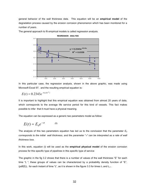
The general approach to fit empirical models is called regression analysis.<br />
0.27<br />
REGRESSION ANALYSIS<br />
0.25<br />
0.23<br />
y = 0.2343e -3E-05x<br />
R 2 = 0.6359<br />
0.21<br />
0.19<br />
0.17<br />
0.15<br />
0 1000 2000 3000 4000 5000 6000 7000<br />
In this particular case, the regression analysis, shown in the above graphic, was made using<br />
Micros<strong>of</strong>t Excel 97, and the resulting empirical equation is:<br />
E(<br />
t)<br />
= 0.2343e<br />
−8x10<br />
−6<br />
t<br />
It is important to highlight that this empirical equation was obtained from almost 20 years <strong>of</strong> data,<br />
which corresponds to the average life service period for this kind <strong>of</strong> vessels. This fact makes<br />
possible to infer that it must have a physical meaning.<br />
The equation can be expressed as a generic two parameters model as follow:<br />
E(<br />
t)<br />
= E 0<br />
e<br />
−υt<br />
(i)<br />
The analysis <strong>of</strong> this two parameters equation has led us to the conclusion that the parameter E 0<br />
corresponds to the initial wall thickness, and the parameter “ν” can be interpreted as a rate <strong>of</strong> wall<br />
thickness loss.<br />
In this work, equation (i) will be used as the empirical physical model <strong>of</strong> the erosion corrosion<br />
process for this specific type <strong>of</strong> pipelines in this specific type <strong>of</strong> service<br />
The graphic in the fig 3.2 shows that there is a number <strong>of</strong> values <strong>of</strong> the wall thickness “E” for each<br />
time “t i “; these groups <strong>of</strong> values can be characterized by a probability density function <strong>of</strong> “E”,<br />
(pdf(E)), for each instant <strong>of</strong> time “t i “, as it is shown in the figure 3.3 for times t 1 and t n-1 .<br />
32