Remaining Life of a Pipeline

The method to find the most suitable probability distribution function of “E”, ( pdf(E)) will be described
in step #3.
In a similar fashion, the limit wall thickness “E lim “ which has been traditionally considered as a
deterministic value, can also be considered as having its own probability distribution, as the one
shown in the figure 3.4.These procedure will be further explained in step #2
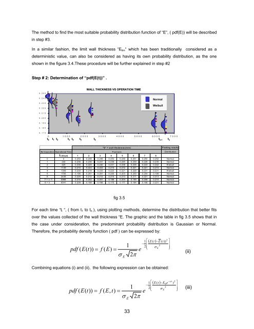
Step # 2: Determination of “pdf(E(t))” .
0.255
WALL THICKNESS VS OPERATION TIME
0.245
0.235
0.225
Normal
Weibull
0.215
0.205
0.195
0.185
0.175
0 1000 2000 3000 4000 5000 6000 7000
t 0 t 1 t 2 t 3 t 4 t 5 t 6
t n-1
t n
"E" = wall thickness (mm)
Plotting results
No Inspection Operational Tim e Positions
Distribution
ti (days) 1 2 3 4 5 6 7 8
0 0 0.250 0.248 0.248 0.253 0.248 0.251 0.250 0.252 Normal
1 240 0.236 0.236 0.241 0.236 0.245 0.239 0.226 0.235 Normal
2 425 0.236 0.225 0.240 0.231 0.236 0.238 0.243 0.242 W eibull
3 1139 0.215 0.223 0.223 0.215 0.212 0.221 0.221 0.215 Normal
4 1309 0.230 0.218 0.233 0.223 0.221 0.228 0.231 0.231 W eibull
5 1706 0.196 0.201 0.201 0.200 0.203 0.209 0.204 0.199 Normal
6 2436 0.225 0.212 0.212 0.215 0.213 0.211 0.221 0.213 Normal
7 = n -1 5968 0.216 0.202 0.201 0.188 0.204 0.199 0.208 0.210 Normal
8 = n 6541 0.208 0.198 0.188 0.175 0.177 0.184 0.198 0.201 Normal
fig 3.5
For each time “t i “, ( from t 1 to t n ), using plotting methods, determine the distribution that better fits
over the values collected of the wall thickness “E. The graphic and the table in fig 3.5 shows that in
the case under consideration, the predominant probability distribution is Gaussian or Normal.
Therefore, the probability density function ( pdf ) can be expressed by:
pdf
1
E(
t))
= f ( E)
=
σ 2π
1 ⎡
− ⎢
2 ⎢⎣
( E(
t )
2
σ E
( e
E
−E
( t))
2
⎤
⎥
⎥⎦
(ii)
Combining equations (i) and (ii), the following expression can be obtained:
pdf
1 ⎡
− ⎢
2 ⎢⎣
( E(
t )
−υt
2
−E0 e )
1
2
σ E
( E(
t))
= f ( E,
t)
= e
σ
E
2π
⎤
⎥
⎥⎦
(iii)
33