Remaining Life of a Pipeline

This method can be applied for any value of the time “t” in order to estimate the mean and the
variance of the failure pressure or remaining strength. Table 2 shows the results gotten for t =
20,30,40 and 50 years
Time “t” (years) µ Pf (Mpa) σ Pf (Mpa) cov=σ Pf/ µ Pf
20 10.527 1.259 0.1196
30 8.917 1.547 0.1734
40 7.102 1.978 0.2785
50 5.044 2.57 0.5095
table 2
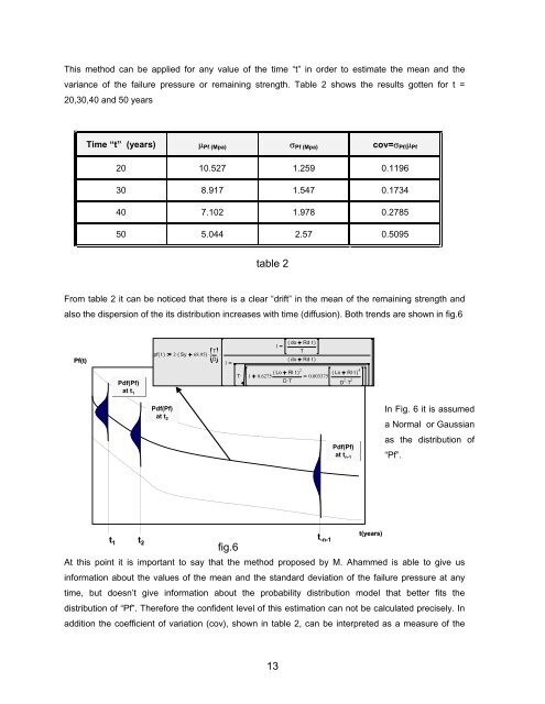
From table 2 it can be noticed that there is a clear “drift” in the mean of the remaining strength and
also the dispersion of the its distribution increases with time (diffusion). Both trends are shown in fig.6
Pf(t)
Pdf(Pf)
at t 1
pf( t ) 2. ( Sy 68.95)
. T .
D
1
1
( do Rd.
t )
T
( do Rd.
t )
Lo Rl.
T.
( t ) 2
1 0.6275. DT . 0.003375.
( Lo Rl.
t ) 4
D 2 . T 2
Pdf(Pf)
at t 2
Pdf(Pf)
at t n-1
In Fig. 6 it is assumed
a Normal or Gaussian
as the distribution of
“Pf”.
t 1 t 2
fig.6
At this point it is important to say that the method proposed by M. Ahammed is able to give us
information about the values of the mean and the standard deviation of the failure pressure at any
time, but doesn’t give information about the probability distribution model that better fits the
distribution of “Pf”. Therefore the confident level of this estimation can not be calculated precisely. In
addition the coefficient of variation (cov), shown in table 2, can be interpreted as a measure of the
t -n-1
t(years)
13