Remaining Life of a Pipeline

You also want an ePaper? Increase the reach of your titles
YUMPU automatically turns print PDFs into web optimized ePapers that Google loves.
β<br />
( Pf Pa )<br />
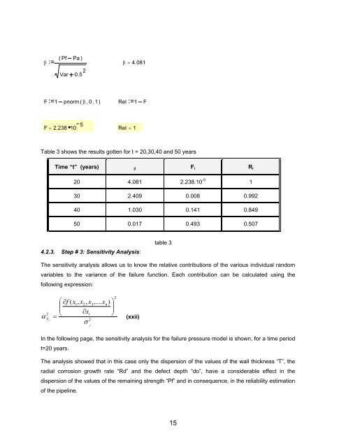
β = 4.081<br />
Var 0.5 2<br />
F 1 pnorm ( β , 0 , 1 ) Rel 1 F<br />
F = 2.238 10 5<br />
Rel = 1<br />
Table 3 shows the results gotten for t = 20,30,40 and 50 years<br />
Time “t” (years) β F i R i<br />
20 4.081 2.238.10 -5 1<br />
30 2.409 0.008 0.992<br />
40 1.030 0.141 0.849<br />
50 0.017 0.493 0.507<br />
4.2.3. Step # 3: Sensitivity Analysis:<br />
table 3<br />
The sensitivity analysis allows us to know the relative contributions <strong>of</strong> the various individual random<br />
variables to the variance <strong>of</strong> the failure function. Each contribution can be calculated using the<br />
following expression:<br />
α<br />
2<br />
X<br />
i<br />
=<br />
⎛ ∂f<br />
( x1,<br />
x2,<br />
x3,....<br />
x<br />
⎜<br />
⎝ ∂xi<br />
2<br />
σ<br />
f<br />
n<br />
) ⎞<br />
⎟<br />
⎠<br />
2<br />
(xxii)<br />
In the following page, the sensitivity analysis for the failure pressure model is shown, for a time period<br />
t=20 years.<br />
The analysis showed that in this case only the dispersion <strong>of</strong> the values <strong>of</strong> the wall thickness “T”, the<br />
radial corrosion growth rate “Rd” and the defect depth “do”, have a considerable effect in the<br />
dispersion <strong>of</strong> the values <strong>of</strong> the remaining strength “Pf” and in consequence, in the reliability estimation<br />
<strong>of</strong> the pipeline.<br />
15