WRF ARW User's Guide - MMM - UCAR

�� 

�� 10 

��

Foreword 

This User’s Guide describes the Advanced Research WRF (ARW) Version 3.1 modeling 

system, released in April 2009. As the ARW is developed further, this document will be 

continuously enhanced and updated. 

This document is complimentary to the ARW Tech Note 

(http://www.mmm.ucar.edu/wrf/users/docs/arw_v3.pdf), which describes the equations, 

numerics, boundary conditions, and nesting etc. in greater detail. 

Highlights of updates to WRFV3.1 include: 

• Monotonic transport option 

• Gravity wave drag 

• Spectral nudging 

• Surface analysis nudging 

• Noah LSM modifications and multi-layer urban canopy model (BEP: Building 

Environment Parameterization) 

• New physics options: 

o QNSE (Quasi-Normal Scale Elimination), MYNN (Mellor-Yamada Nakanishi- 

Niino) and BouLac (Bougeault and Lacarrere) PBL schemes 

o New RRTM long- and short-wave radiation schemes 

o Modifications for regional climate applications 

o YSU WRF double moment microphysics schemes 

o New Thompson microphysics 

• Polar modifications 

o Fractional sea ice and Noah LSM modifications 

• Single Column model 

• WRF-Chem updates 

• WRF NMM operational (NCEP) code physics and dynamics 

• WRF-Var 

o Radiance assimilation 

o 4DVAR 

• MODIS landuse data for Noah 

• Software framework enhancements 

For the latest version of this document, please visit the ARW Users’ Web site at 

http://www.mmm.ucar.edu/wrf/users/. 

Please send feedback to wrfhelp@ucar.edu. 

Contributors to this guide: 

Wei Wang, Cindy Bruyère, Michael Duda, Jimy Dudhia, Dave Gill, Hui-Chuan Lin, John 

Michalakes, Syed Rizvi, and Xin Zhang

1. Overview 

− Introduction ................................................................................. 1-1 

− The WRF Modeling System Program Components ..................... 1-2 

2. Software Installation 

− Introduction .................................................................................. 2-1 

− Required Compilers and Scripting Languages............................. 2-2 

− Required/Optional Libraries to Download..................................... 2-2 

− Post-Processing Utilities............................................................... 2-3 

− Unix Environment Settings........................................................... 2-4 

− Building the WRF Code................................................................ 2-5 

− Building the WPS Code................................................................ 2-6 

− Building the WRF VAR Code ....................................................... 2-7 

3. The WRF Preprocessing System (WPS) 

− Introduction ................................................................................. 3-1 

− Function of Each WPS Program ................................................. 3-2 

− Installing the WPS....................................................................... 3-4 

− Running the WPS........................................................................ 3-7 

− Creating Nested Domains with the WPS................................... 3-18 

− Selecting Between USGS and MODIS-based 

Land Use Classifications........................................................... 3-20 

− Selecting Static Data for the Gravity Wave Drag Scheme ........ 3-21 

− Using Multiple Meteorological Data Sources............................. 3-22 

− Parallelism in the WPS.............................................................. 3-25 

− Checking WPS Output .............................................................. 3-26 

− WPS Utility Programs................................................................ 3-27 

− Writing Meteorological Data to the Intermediate Format ........... 3-30 

− Creating and Editing Vtables..................................................... 3-32 

− Writing Static Data to the Geogrid Binary Format ..................... 3-34 

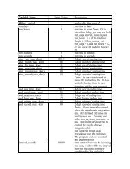
− Description of Namelist Variables ............................................. 3-37 

− Description of GEOGRID.TBL Options ..................................... 3-42 

− Description of index Options ..................................................... 3-45 

− Description of METGRID.TBL Options...................................... 3-48 

− Available Interpolation Options in Geogrid and Metgrid ............ 3-51 

− Land Use and Soil Categories in the Static Data ...................... 3-54 

− WPS Output Fields.................................................................... 3-56 

4. WRF Initialization 

− Introduction ................................................................................. 4-1 

− Initialization for Ideal Data Cases................................................ 4-3 

− Initialization for Real Data Cases ................................................ 4-5 

CONTENTS 

WRF-ARW V3: User’s Guide i

CONTENTS 

5. WRF Model 

− Introduction ................................................................................ 5-1 

− Installing WRF ............................................................................5-2 

− Running WRF .............................................................................5-7 

− Check Output ........................................................................... 5-22 

− Trouble Shooting....................................................................... 5-23 

− Physics and Dynamics Options................................................. 5-24 


− WRF Output Fields.................................................................... 5-53 

6. WRF-Var 

− Introduction ................................................................................. 6-1 

− Installing WRF-Var …. ................................................................ 6-3 

− Installing WRFNL and WRFPLUS............................................... 6-6 

− Running Observation Preprocessor (OBSPROC) ...................... 6-7 

− Running WRF-Var..................................................................... 6-12 

− Radiance Data Assimilations in WRF-Var................................. 6-20 

− WRF-Var Diagnostics................................................................ 6-29 

− Updating WRF boundary conditions.......................................... 6-33 

− Running gen_be........................................................................ 6-34 

− Additional WRF-Var Exercises.................................................. 6-37 


7. Objective Analysis (OBSGRID) 

− Introduction ................................................................................. 7-1 

− Program Flow..............................................................................7-2 

− Source of Observations............................................................... 7-3 

− Objective Analysis techniques in OBSGRID ............................... 7-3 

− Quality Control for Observations ................................................. 7-5 

− Additional Observations .............................................................. 7-6 

− Surface FDDA option .................................................................. 7-6 

− Objective Analysis on Model Nests............................................. 7-7 

− How to run OBSGRID ................................................................. 7-7 

− Output Files.................................................................................7-9 

− Plot Utilities ............................................................................... 7-11 

− Observations Format................................................................. 7-12 

− OBSGRID Namelist................................................................... 7-15 

WRF-ARW V3: User’s Guide ii

8. WRF Software 

− Introduction ................................................................................. 8-1 

− WRF Build Mechanism................................................................ 8-1 

− Registry....................................................................................... 8-4 

− I/O Applications Program Interface (I/O API) ............................ 8-14 

− Timekeeping ............................................................................. 8-14 

− Software Documentation........................................................... 8-15 

− Portability and Performance...................................................... 8-15 

9. Post-Processing Programs 

− Introduction ................................................................................. 9-1 

− NCL.. .......................................................................................... 9-2 

− RIP4 . ........................................................................................ 9-19 

− ARWpost................................................................................... 9-28 

− WPP ........................................................................................9-35 

− VAPOR ..................................................................................... 9-50 

10. Utilities and Tools 

− Introduction ............................................................................... 10-1 

− read_wrf_nc .............................................................................. 10-1 

− iowrf . ........................................................................................ 10-5 

− p_interp ..................................................................................... 10-6 

− TC Bogus Scheme .................................................................... 10-8 

− v_interp ................................................................................... 10-10 

− Tools ...................................................................................... 10-12 

CONTENTS 

WRF-ARW V3: User’s Guide iii

CONTENTS 

WRF-ARW V3: User’s Guide iv

Table of Contents 

Chapter 1: Overview 

• Introduction 

• The WRF ARW Modeling System Program Components 

Introduction 

OVERVIEW 

The Advanced Research 

WRF (ARW) modeling system has been in development for the 

past few years. The current release is Version 3, available since April 2008. The ARW is 

designed to be a flexible, state-of-the-art atmospheric simulation system that is portable 

and efficient on available parallel computing platforms. The ARW is suitable for use in a 

broad range of applications across scales ranging from meters to thousands of kilometers, 

including: 

• Idealized 

simulations (e.g. LES, convection, baroclinic waves) 

• Parameterization research 

• Data assimilation research 

• Forecast research 

• Real-time NWP 

• Coupled-model applications 

• Teaching 

The Mesoscale and 

Microscale Meteorology Division of NCAR is currently maintaining 

and supporting a subset of the overall WRF code (Version 3) that includes: 

• WRF Software Framework (WSF) 

• Advanced Research WRF (ARW) dynamic 

solver, including one-way, two-way 

nesting and moving nest. 

• The WRF Preprocessing System (WPS) 

• WRF Variational Data Assimilation (WRF-Var) 

system which currently supports 

3DVAR capability 

• Numerous physics packages contributed by WRF partners and the research 

community 

• Several graphics programs and conversion programs for other graphics tools 

And these are the subjects of this document. 

The WRF modeling system software is in the 

community use. 

public domain and is freely available for 

WRF-ARW V3: User’s Guide 1-1

OVERVIEW 

The WRF Modeling System Program Components 

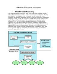
The following figure shows the flowchart for the WRF Modeling System Version 3. 

As shown in the diagram, the WRF Modeling System consists of these major programs: 

WPS 

• The WRF Preprocessing System (WPS) 

• WRF-Var 

• ARW solver 

• Post-processing & Visualization tools 

This program is used primarily for real-data simulations. Its functions include 1) defining 

simulation domains; 2) interpolating terrestrial data (such as terrain, landuse, and soil 

types) to the simulation domain; and 3) degribbing and interpolating meteorological data 

from another model to this simulation domain. Its main features include: 

• GRIB 1/2 meteorological data from various centers around the world 


OVERVIEW 

• Map projections for 1) polar stereographic, 2) Lambert-Conformal, 3) Mercator and 

4) latitude-longitude 

• Nesting 

• User-interfaces to input other static data as well as met data 

WRF-Var 

This program is optional, but can be used to ingest observations into the interpolated 

analyses created by WPS. It can also be used to update WRF model's initial condition 

when WRF model is run in cycling mode. Its main features are as follows. 

• It is based on incremental variational data assimilation technique 

• Conjugate gradient method is utilized to minimized the cost function in analysis 

control variable space 

• Analysis is performed on un-staggered Arakawa A-grid 

• Analysis increments are interpolated to staggered Arakawa C-grid and it gets added to 

the background (first guess) to get final analysis at WRF-model grid 

• Conventional observation data input may be supplied both in ASCII or “PREPBUFR” 

format via “obsproc” utility 

• Multiple radar data (reflectivity & radial velocity) input is supplied through ASCII 

format 

• Horizontal component of the background (first guess) error is represented via 

recursive filter (for regional) or power spectrum (for global). The vertical component 

is applied through projections on climatologically generated averaged eigenvectors 

and its corresponding eigenvalues 

• Horizontal and vertical background errors are non-separable. Each eigen vector has 

its own horizontal climatologically determined length scale 

• Preconditioning of background part of the cost function is done via control variable 

transform U defined as B= UU T 

• It includes “gen_be” utility to generate the climatological background error 

covariance estimate via the NMC-method or ensemble perturbations 

• A utility program to update WRF boundary condition file after WRF-Var 

ARW Solver 

This is the key component of the modeling system, which is composed of several 

initialization programs for idealized, and real-data simulations, and the numerical 

integration program. It also includes a program to do one-way nesting. The key feature of 

the WRF model includes: 

• Fully compressible nonhydrostatic equations with hydrostatic option 

• Regional and global applications 

• Complete coriolis and curvature terms 

• Two-way nesting with multiple nests and nest levels 

• One-way nesting 


OVERVIEW 

• Moving nests 

• Mass-based terrain following coordinate 

• Vertical grid-spacing can vary with height 

• Map-scale factors for these projections: 

o polar stereographic (conformal) 

o Lambert-conformal 

o Mercator (conformal) 

o Latitude and longitude which can be rotated 

• Arakawa C-grid staggering 

• Runge-Kutta 2nd and 3rd order time integration options 

• Scalar-conserving flux form for prognostic variables 

• 2nd to 6th order advection options (horizontal and vertical) 

• Monotonic transport and positive-definite advection option for moisture, scalar and 

TKE 

• Time-split small step for acoustic and gravity-wave modes: 

o small step horizontally explicit, vertically implicit 

o divergence damping option and vertical time off-centering 

o external-mode filtering option 

• Upper boundary aborption and Rayleigh damping 

• Lateral boundary conditions 

o idealized cases: periodic, symmetric, and open radiative 

o real cases: specified with relaxation zone 

• Full physics options for land-surface, planetary boundary layer, atmospheric and 

surface radiation, microphysics and cumulus convection 

• Grid analysis nudging using separate upperair and surface data and observation 

nudging 

• Spectral nudging 

• Digital filter initialization 

• Gravity wave drag 

• A number of idealized examples 

Graphics and Verification Tools 

Several programs are supported, including RIP4 (based on NCAR Graphics), NCAR 

Graphics Command Language (NCL), and conversion programs for other readily 

available graphics packages: GrADS and Vis5D. 

Program VAPOR, Visualization and Analysis Platform for Ocean, Atmosphere, and 

Solar Researchers (http://www.vapor.ucar.edu/), is a 3-dimensional data visualization 

tool, and it is developed and supported by the VAPOR team at NCAR (vapor@ucar.edu). 

Program MET, Model Evaluation Tools (http://www.dtcenter.org/met/users/), is 

developed and supported by the Developmental Testbed Center at NCAR 

(met_help@ucar.edu). 

The details of these programs are described more in the chapters in this user's guide. 



Chapter 2: Software Installation 


• Required Compilers and Scripting Languages 

• Required/Optional Libraries to Download 

• Post-Processing Utilities 

• UNIX Environment Settings 

• Building the WRF Code 

• Building the WPS Code 

• Building the WRF-Var Code 

Introduction 

SOFTWARE INSTALLATION 

The WRF modeling system software installation is fairly straightforward on the ported 

platforms listed below. The model-component portion of the package is mostly selfcontained. 

The WRF model does contain the source code to a Fortran interface to ESMF 

and the source to FFTPACK . Contained within the WRF system is the WRF-Var 

component, which has several external libraries that the user must install (for various 

observation types and linear algebra solvers). Similarly, the WPS package, separate from 

the WRF source code, has additional external libraries that must be built (in support of 

Grib2 processing). The one external package that all of the systems require is the 

netCDF library, which is one of the supported I/O API packages. The netCDF libraries or 

source code are available from the Unidata homepage at http://www.unidata.ucar.edu 

(select DOWNLOADS, registration required). 

There are three tar files for the WRF code. The first is the WRF model (including the 

real and ideal pre-processors). The second is the WRF-Var code. The third tar file is for 

WRF chemistry. In order to run the WRF chemistry code, both the WRF model and the 

chemistry tar file must be combined. 

The WRF model has been successfully ported to a number of Unix-based machines. We 

do not have access to all of them and must rely on outside users and vendors to supply the 

required configuration information for the compiler and loader options. Below is a list of 

the supported combinations of hardware and software for WRF. 

Vendor Hardware OS Compiler 

Cray X1 UniCOS vendor 

Cray AMD Linux PGI / 



PathScale 

IBM Power Series AIX vendor 

SGI IA64 / Opteron Linux Intel 

COTS* IA32 Linux 

COTS IA64 / Opteron Linux 

Intel / PGI / 

gfortran / g95 / 

PathScale 

Intel / PGI / 

gfortran / 

PathScale 

Mac Power Series Darwin xlf / g95 / PGI / Intel 

Mac Intel Darwin 

* Commercial Off The Shelf systems 

g95 / PGI / Intel 

The WRF model may be built to run on a single processor machine, a shared-memory 

machine (that use the OpenMP API), a distributed memory machine (with the appropriate 

MPI libraries), or on a distributed cluster (utilizing both OpenMP and MPI). The WRF- 

Var and WPS packages run on the above listed systems. 

Required Compilers and Scripting Languages 

The majority of the WRF model, WPS, and WRF-Var codes are written in Fortran (what 

many refer to as Fortran 90). The software layer, RSL_LITE, which sits between WRF 

and WRF-Var and the MPI interface is written in C. WPS makes direct calls to the MPI 

libraries for distributed memory message passing. There are also ancillary programs that 

are written in C to perform file parsing and file construction, which are required for 

default building of the WRF modeling code. Additionally, the WRF build mechanism 

uses several scripting languages: including perl, Cshell and Bourne shell. The traditional 

UNIX text/file processing utilities are used: make, m4, sed, and awk. See Chapter 8: 

WRF Software (Required Software) for a more detailed listing of the necessary pieces for 

the WRF build. 

Required/Optional Libraries to Download 

The only library that is almost always required is the netCDF package from Unidata 

(login > Downloads > NetCDF). Most of the WRF post-processing packages assume that 

the data from the WRF model, the WPS package, or the WRF-Var program is using the 

netCDF libraries. One may also need to add /path-to-netcdf/netcdf/bin to your path so 

that one may execute netCDF utility commands, such as ncdump. 



Note 1: If one wants to compile WRF system components on a Linux system that has 

access to multiple compilers, link the correct external libraries. For example, do not link 

the libraries built with PathScale when compiling the WRF components with gfortran. 

Note 2: If netCDF-4 is used, be sure that it is installed without activating the new 

capabilities (such as parallel I/O based on HDF5). The WRF modeling system currently 

only uses its classic data model supported in netCDF-4. 

If you are going to be running distributed memory WRF jobs, you need a version of MPI. 

You can pick up a version of mpich, but you might want your system group to install the 

code. A working installation of MPI is required prior to a build of WRF using distributed 

memory. Either MPI-1 or MPI-2 are acceptable. Do you already have an MPI lying 

around? Try 

which mpif90 

which mpicc 

which mpirun 

If these are all defined executables in your path, you are probably OK. Make sure your 

paths are set up to point to the MPI lib, include, and bin directories. 

Note that to output WRF model data in Grib1 format, Todd Hutchinson (WSI) has 

provided a complete source library that is included with the software release. However, 

when trying to link the WPS, the WRF model, and the WRF-Var data streams together, 

always use the netCDF format. 

Post-Processing Utilities 

The more widely used (and therefore supported) WRF post-processing utilities are: 

• NCL (homepage and WRF download) 

o NCAR Command Language written by NCAR Scientific Computing 

Division 

o NCL scripts written and maintained by WRF support 

o many template scripts are provided that are tailored for specific real-data 

and ideal-data cases 

o raw WRF output can be input with the NCL scripts 

o interactive or command-file driven 

• Vis5D (homepage and WRF download) 

o download Vis5D executable, build format converter 

o programs are available to convert the WRF output into an input format 

suitable for Vis5D 

o GUI interface, 3D movie loops, transparency 



• GrADS (homepage and WRF download) 

o download GrADS executable, build format converter 

o programs are available to convert the WRF output into an input format 

suitable for GrADS 

o interpolates to regular lat/lon grid 

o simple to generate publication quality 

• RIP (homepage and WRF download) 

o RIP4 written and maintained by Mark Stoelinga, UW 

o interpolation to various surfaces, trajectories, hundreds of diagnostic 

calculations 

o Fortran source provided 

o based on the NCAR Graphics package 

o pre-processor converts WRF, WPS, and WRF-Var data to RIP input 

format 

o table driven 

UNIX Environment Settings 

There are only a few environmental settings that are WRF system related. Most of these 

are not required, but when things start acting badly, test some out. In Cshell syntax: 

• setenv WRF_EM_CORE 1 

o explicitly defines which model core to build 

• setenv WRF_NMM_CORE 0 

o explicitly defines which model core NOT to build 

• setenv WRF_DA_CORE 0 

o explicitly defines no data assimilation 

• setenv NETCDF /usr/local/netcdf (or where ever you have it stuck) 

o all of the WRF components want both the lib and the include directories 

• setenv OMP_NUM_THREADS n (where n is the number of procs to use) 

o if you have OpenMP on your system, this is how to specify the number of 

threads 

• setenv MP_STACK_SIZE 64000000 

o OpenMP blows through the stack size, set it large. 

o However, if the model still crashes, it may be a problem of over specifying 

stack size. Set stack size sufficiently large, but not unlimited. 

o On some system, the equivalent parameter could be KMP_STACKSIZE, 

or OMP_STACKSIZE. 

• unlimit 

o especially if you are on a small system 


Building the WRF Code 


The WRF code has a fairly complicated build mechanism. It tries to determine the 

architecture that you are on, and then presents you with options to allow you to select the 

preferred build method. For example, if you are on a Linux machine, it determines 

whether this is a 32 or 64 bit machine, and then prompts you for the desired usage of 

processors (such as serial, shared memory, or distributed memory). You select from 

among the available compiling options in the build mechanism. For example, do not 

choose a PGI build if you do not have PGI compilers installed on your system. 

• Get the WRF zipped tar file from WRFV3 from 

o http://www.mmm.ucar.edu/wrf/users/download/get_source.html 

o always get the latest version if you are not trying to continue a long project 

• unzip and untar the file 

o gzip -cd WRFV3.TAR.gz | tar -xf - 

• cd WRFV3 

• ./configure 

o serial means single processor 

o smpar means Symmetric Multi-Processing/Shared Memory Parallel 

(OpenMP) 

o dmpar means Distributed Memory Parallel (MPI) 

o dm+sm means Distributed Memory with Shared Memory (for example, 

MPI across nodes with OpenMP within a node) 

o the second option is for nesting: 0 = no nesting, 1 = standard static nesting, 

2 = nesting with a prescribed set of moves, 3 = nesting that allows a 

domain to follow a vortex (typhoon tracking) 

• ./compile em_real (or any of the directory names in ./WRFV3/test 

directory) 

• ls -ls main/*.exe 

o if you built a real-data case, you should see ndown.exe, real.exe, and 

wrf.exe 

o if you built an ideal-data case, you should see ideal.exe and wrf.exe 

Users wishing to run the WRF chemistry code must first download the WRF model tar 

file, and untar it. Then the chemistry code is untar’ed in the WRFV3 directory (this is the 

chem directory structure). Once the source code from the tar files is combined, then 

users may proceed with the WRF chemistry build. 



Building the WPS Code 

Building WPS requires that WRFV3 is already built. 

• Get the WPS zipped tar file WPSV3.TAR.gz from 

o http://www.mmm.ucar.edu/wrf/users/download/get_source.html 

• Also download the geographical dataset from the same page 

• unzip and untar the file 

o gzip -cd WPSV3.TAR.gz | tar -xf - 

• cd WPS 

• ./configure 

o choose one of the options 

o usually, option "1" and option “2” are for serial builds, that is the best for 

an initial test 

o WPS requires that you build for the appropriate Grib decoding, select an 

option that suitable for the data you will use with the ungrib program 

o If you select a Grib2 option, you must have those libraries prepared and 

built in advance 

• ./compile 

• ls -ls *.exe 

o you should see geogrid.exe, ungrib.exe, and metgrid.exe (if 

you are missing both geogrid.exe and metgrid.exe, you probably 

need to fix where the path to WRF is pointing in the configure.wps 

file; if you are missing ungrib.exe, try a Grib1-only build to further 

isolate the problem) 

• ls -ls util/*.exe 

o you should see a number of utility executables: avg_tsfc.exe, 

calc_ecmwf_p.exe, g1print.exe, g2print.exe, 

mod_levs.exe, plotfmt.exe, plotgrids.exe, and 

rd_intermediate.exe (files requiring NCAR Graphics are 

plotfmt.exe and plotgrids.exe) 

• if geogrid.exe and metgrid.exe executables are missing, probably the 

path to the WRFV3 directory structure is incorrect (found inside the 

configure.wps file) 

• if the ungrib.exe is missing, probably the Grib2 libraries are not linked or 

built correctly 

• if the plotfmt.exe or the plotgrids.exe programs are missing, probably 

the NCAR Graphics path is set incorrectly 


Building the WRF-Var Code 


WRF-Var uses the same build mechanism as WRF, and as a consequence, this 

mechanism must be instructed to configure and build the code for WRF-Var rather than 

WRF. Additionally, the paths to libraries needed by WRF-Var code must be set, as 

described in the steps below. 

• Get the WRF-Var zipped tar file, WRFDAV3_1_1.TAR.gz, from 

http://www.mmm.ucar.edu/wrf/users/download/get_source.html 

• Unzip and untar the WRF-Var code 

o gzip -cd WRFDAV3_1_1.TAR.gz | tar -xf – 

o This will create a directory, WRFDA 

• cd WRFDA 

o In addition to NETCDF, set up environment variables pointing to 

additional libraries required by WRF-Var. 

o If you intend to use PREPBUFR observation data from NCEP, 

environment variable BUFR has to be set with 

setenv BUFR 1 

o If you intend to use satellite radiance data, either CRTM (V1.2) or 

RTTOV (V8.7) has to be installed. They can be downloaded from 

ftp://ftp.emc.ncep.noaa.gov/jcsda/CRTM/ and 

http://www.metoffice.gov.uk/science/creating/work 

ing_together/nwpsaf_public.html 

• Make certain that all the required libraries are compiled using the same compiler 

as will be used to build WRF-Var, since the libraries produced by one compiler 

may not be compatible with code compiled with another. 

• Assuming, for example, that these libraries have been installed in subdirectories 

of /usr/local, the necessary environment variables might be set with 

o setenv CRTM /usr/local/crtm (optional, make sure 

libcrtm.a is in $CRTM directory) 

o setenv RTTOV /usr/local/rttov87 (optional, make 

sure librttov.a is in $RTTOV directory) 

• ./configure wrfda 

o serial means single processor 

o smpar means Symmetric Multi-Processing/Shared Memory Parallel 

(OpenMP) 

o dmpar means Distributed Memory Parallel (MPI) 

o dm+sm means Distributed Memory with Shared Memory (for example, 

MPI across nodes with OpenMP within a node) 

• ./compile all_wrfvar 



• ls -ls var/build/*.exe 

o If the compilation was successful, da_wrfvar.exe, 

da_update_bc.exe, and other executables should be found in the 

var/build directory and their links are in var/da directory; obsproc.exe 

should be found in the var/obsproc/src directory 


Chapter 3: WRF Preprocessing System (WPS) 



• Function of Each WPS Program 

• Installing the WPS 

• Running the WPS 

• Creating Nested Domains with the WPS 

• Selecting Between USGS and MODIS-based Land Use Data 

• Selecting Static Data for the Gravity Wave Drag Scheme 

• Using Multiple Meteorological Data Sources 

• Parallelism in the WPS 

• Checking WPS Output 

• WPS Utility Programs 

• Writing Meteorological Data to the Intermediate Format 

• Creating and Editing Vtables 

• Writing Static Data to the Geogrid Binary Format 

• Description of Namelist Variables 

• Description of GEOGRID.TBL Options 

• Description of index Options 

• Description of METGRID.TBL Options 

• Available Interpolation Options in Geogrid and Metgrid 

• Land Use and Soil Categories in the Static Data 

• WPS Output Fields 

Introduction 

WPS 

The WRF Preprocessing System (WPS) is a set of three programs whose collective role is 

to prepare input to the real program for real-data simulations. Each of the programs 

performs one stage of the preparation: geogrid defines model domains and interpolates 

static geographical data to the grids; ungrib extracts meteorological fields from GRIBformatted 

files; and metgrid horizontally interpolates the meteorological fields extracted 

by ungrib to the model grids defined by geogrid. The work of vertically interpolating 

meteorological fields to WRF eta levels is performed within the real program. 


WPS 

The data flow between the programs of the WPS is shown in the figure above. Each of 

the WPS programs reads parameters from a common namelist file, as shown in the figure. 

This namelist file has separate namelist records for each of the programs and a shared 

namelist record, which defines parameters that are used by more than one WPS program. 

Not shown in the figure are additional table files that are used by individual programs. 

These tables provide additional control over the programs’ operation, though they 

generally do not need to be changed by the user. The GEOGRID.TBL, METGRID.TBL, 

and Vtable files are explained later in this document, though for now, the user need not 

be concerned with them. 

The build mechanism for the WPS, which is very similar to the build mechanism used by 

the WRF model, provides options for compiling the WPS on a variety of platforms. 

When MPICH libraries and suitable compilers are available, the metgrid and geogrid 

programs may be compiled for distributed memory execution, which allows large model 

domains to be processed in less time. The work performed by the ungrib program is not 

amenable to parallelization, so ungrib may only be run on a single processor. 

Function of Each WPS Program 

The WPS consists of three independent programs: geogrid, ungrib, and metgrid. Also 

included in the WPS are several utility programs, which are described in the section on 

utility programs. A brief description of each of the three main programs is given below, 

with further details presented in subsequent sections. 

Program geogrid 

The purpose of geogrid is to define the simulation domains, and interpolate various 

terrestrial data sets to the model grids. The simulation domains are defined using 


WPS 

information specified by the user in the “geogrid” namelist record of the WPS namelist 

file, namelist.wps. In addition to computing the latitude, longitude, and map scale factors 

at every grid point, geogrid will interpolate soil categories, land use category, terrain 

height, annual mean deep soil temperature, monthly vegetation fraction, monthly albedo, 

maximum snow albedo, and slope category to the model grids by default. Global data sets 

for each of these fields are provided through the WRF download page, and, because these 

data are time-invariant, they only need to be downloaded once. Several of the data sets 

are available in only one resolution, but others are made available in resolutions of 30", 

2', 5', and 10'; here, " denotes arc seconds and ' denotes arc minutes. The user need not 

download all available resolutions for a data set, although the interpolated fields will 

generally be more representative if a resolution of data near to that of the simulation 

domain is used. However, users who expect to work with domains having grid spacings 

that cover a large range may wish to eventually download all available resolutions of the 

static terrestrial data. 

Besides interpolating the default terrestrial fields, the geogrid program is general enough 

to be able to interpolate most continuous and categorical fields to the simulation domains. 

New or additional data sets may be interpolated to the simulation domain through the use 

of the table file, GEOGRID.TBL. The GEOGRID.TBL file defines each of the fields that 

will be produced by geogrid; it describes the interpolation methods to be used for a field, 

as well as the location on the file system where the data set for that field is located. 

Output from geogrid is written in the WRF I/O API format, and thus, by selecting the 

NetCDF I/O format, geogrid can be made to write its output in NetCDF for easy 

visualization using external software packages, including ncview, NCL, and the new 

release of RIP4. 

Program ungrib 

The ungrib program reads GRIB files, "degribs" the data, and writes the data in a simple 

format, called the intermediate format (see the section on writing data to the intermediate 

format for details of the format). The GRIB files contain time-varying meteorological 

fields and are typically from another regional or global model, such as NCEP's NAM or 

GFS models. The ungrib program can read GRIB Edition 1 and, if compiled with a 

"GRIB2" option, GRIB Edition 2 files. 

GRIB files typically contain more fields than are needed to initialize WRF. Both versions 

of the GRIB format use various codes to identify the variables and levels in the GRIB 

file. Ungrib uses tables of these codes – called Vtables, for "variable tables" – to define 

which fields to extract from the GRIB file and write to the intermediate format. Details 

about the codes can be found in the WMO GRIB documentation and in documentation 

from the originating center. Vtables for common GRIB model output files are provided 

with the ungrib software. 

Vtables are provided for NAM 104 and 212 grids, the NAM AWIP format, GFS, the 

NCEP/NCAR Reanalysis archived at NCAR, RUC (pressure level data and hybrid 


WPS 

coordinate data), AFWA's AGRMET land surface model output, ECMWF, and other data 

sets. Users can create their own Vtable for other model output using any of the Vtables as 

a template; further details on the meaning of fields in a Vtable are provided in the section 

on creating and editing Vtables. 

Ungrib can write intermediate data files in any one of three user-selectable formats: WPS 

– a new format containing additional information useful for the downstream programs; SI 

– the previous intermediate format of the WRF system; and MM5 format, which is 

included here so that ungrib can be used to provide GRIB2 input to the MM5 modeling 

system. Any of these formats may be used by WPS to initialize WRF, although the WPS 

format is recommended. 

Program metgrid 

The metgrid program horizontally interpolates the intermediate-format meteorological 

data that are extracted by the ungrib program onto the simulation domains defined by the 

geogrid program. The interpolated metgrid output can then be ingested by the WRF real 

program. The range of dates that will be interpolated by metgrid are defined in the 

“share” namelist record of the WPS namelist file, and date ranges must be specified 

individually in the namelist for each simulation domain. Since the work of the metgrid 

program, like that of the ungrib program, is time-dependent, metgrid is run every time a 

new simulation is initialized. 

Control over how each meteorological field is interpolated is provided by the 

METGRID.TBL file. The METGRID.TBL file provides one section for each field, and 

within a section, it is possible to specify options such as the interpolation methods to be 

used for the field, the field that acts as the mask for masked interpolations, and the grid 

staggering (e.g., U, V in ARW; H, V in NMM) to which a field is interpolated. 

Output from metgrid is written in the WRF I/O API format, and thus, by selecting the 

NetCDF I/O format, metgrid can be made to write its output in NetCDF for easy 

visualization using external software packages, including the new version of RIP4. 

Installing the WPS 

The WRF Preprocessing System uses a build mechanism similar to that used by the WRF 

model. External libraries for geogrid and metgrid are limited to those required by the 

WRF model, since the WPS uses the WRF model's implementations of the WRF I/O 

API; consequently, WRF must be compiled prior to installation of the WPS so that the I/O 

API libraries in the WRF external directory will be available to WPS programs. 

Additionally, the ungrib program requires three compression libraries for GRIB Edition 2 

support; however, if support for GRIB2 data is not needed, ungrib can be compiled 

without these compression libraries. 


Required Libraries 

The only library that is required to build the WRF model is NetCDF. The user can find 

the source code, precompiled binaries, and documentation at the UNIDATA home page 

(http://www.unidata.ucar.edu/software/netcdf/). Most users will select the NetCDF I/O 

option for WPS due to the easy access to utility programs that support the NetCDF data 

format, and before configuring the WPS, users should ensure that the environment 

variable NETCDF is set to the path of the NetCDF installation. 

Where WRF adds a software layer between the model and the communications package, 

the WPS programs geogrid and metgrid make MPI calls directly. Most multi-processor 

machines come preconfigured with a version of MPI, so it is unlikely that users will need 

to install this package by themselves. 

WPS 

Three libraries are required by the ungrib program for GRIB Edition 2 compression 

support. Users are encouraged to engage their system administrators for the installation of 

these packages so that traditional library paths and include paths are maintained. Paths to 

user-installed compression libraries are handled in the configure.wps file by the 

COMPRESSION_LIBS and COMPRESSION_INC variables. 

1) JasPer (an implementation of the JPEG2000 standard for "lossy" compression) 

http://www.ece.uvic.ca/~mdadams/jasper/ 

Go down to “JasPer software”, one of the "click here" parts is the source. 

> ./configure 

> make 

> make install 

Note: The GRIB2 libraries expect to find include files in "jasper/jasper.h", so it may be 

necessary to manually create a "jasper" subdirectory in the "include" directory created by 

the JasPer installation, and manually link header files there. 

2) PNG (compression library for "lossless" compression) 

http://www.libpng.org/pub/png/libpng.html 

Scroll down to "Source code" and choose a mirror site. 

> ./configure 

> make check 


3) zlib (a compression library used by the PNG library) 

http://www.zlib.net/ 

Go to "The current release is publicly available here" section and download. 

> ./configure 

> make 



WPS 

To get around portability issues, the NCEP GRIB libraries, w3 and g2, have been 

included in the WPS distribution. The original versions of these libraries are available for 

download from NCEP at http://www.nco.ncep.noaa.gov/pmb/codes/GRIB2/. The specific 

tar files to download are g2lib and w3lib. Because the ungrib program requires modules 

from these files, they are not suitable for usage with a traditional library option during the 

link stage of the build. 

Required Compilers and Scripting Languages 

The WPS requires the same Fortran and C compilers as were used to build the WRF 

model, since the WPS executables link to WRF's I/O API libraries. After executing the 

./configure command in the WPS directory, a list of supported compilers on the 

current system architecture are presented. 

WPS Installation Steps 

• Download the WPSV3.TAR.gz file and unpack it at the same directory level as 

WRFV3, as shown below. 

> ls 

-rw-r--r-- 1 563863 WPS.TAR.gz 

drwxr-xr-x 18 4096 WRFV3 

> gzip -d WPSV3.TAR.gz 

> tar xf WPSV3.TAR 

> ls 

drwxr-xr-x 7 4096 WPS 

-rw-r--r-- 1 3491840 WPSV3.TAR 

drwxr-xr-x 18 4096 WRFV3 

• At this point, a listing of the current working directory should at least include the 

directories WRFV3 and WPS. First, compile WRF (see the instructions for 

installing WRF). Then, after the WRF executables are generated, change to the 

WPS directory and issue the configure command followed by the compile 

command as below. 

> cd WPS 

> ./configure 

o Choose one of the configure options 

> ./compile >& compile.output 

• After issuing the compile command, a listing of the current working directory 

should reveal symbolic links to executables for each of the three WPS programs: 

geogrid.exe, ungrib.exe, and metgrid.exe. If any of these links do not exist, check 

the compilation output in compile.output to see what went wrong. 


ls 

drwxr-xr-x 2 4096 arch 

-rwxr-xr-x 1 1672 clean 

-rwxr-xr-x 1 3510 compile 

-rw-r--r-- 1 85973 compile.output 

-rwxr-xr-x 1 4257 configure 

-rw-r--r-- 1 2486 configure.wps 

drwxr-xr-x 4 4096 geogrid 

lrwxrwxrwx 1 23 geogrid.exe -> geogrid/src/geogrid.exe 

-rwxr-xr-x 1 1328 link_grib.csh 

drwxr-xr-x 3 4096 metgrid 

lrwxrwxrwx 1 23 metgrid.exe -> metgrid/src/metgrid.exe 

-rw-r--r-- 1 1101 namelist.wps 

-rw-r--r-- 1 1987 namelist.wps.all_options 

-rw-r--r-- 1 1075 namelist.wps.global 

-rw-r--r-- 1 652 namelist.wps.nmm 

-rw-r--r-- 1 4786 README 

drwxr-xr-x 4 4096 ungrib 

lrwxrwxrwx 1 21 ungrib.exe -> ungrib/src/ungrib.exe 

drwxr-xr-x 3 4096 util 

Running the WPS 

There are essentially three main steps to running the WRF Preprocessing System: 

WPS 

1. Define a model coarse domain and any nested domains with geogrid. 

2. Extract meteorological fields from GRIB data sets for the simulation period with 

ungrib. 

3. Horizontally interpolate meteorological fields to the model domains with metgrid. 

When multiple simulations are to be run for the same model domains, it is only necessary 

to perform the first step once; thereafter, only time-varying data need to be processed for 

each simulation using steps two and three. Similarly, if several model domains are being 

run for the same time period using the same meteorological data source, it is not 

necessary to run ungrib separately for each simulation. Below, the details of each of the 

three steps are explained. 

Step 1: Define model domains with geogrid 

In the root of the WPS directory structure, symbolic links to the programs geogrid.exe, 

ungrib.exe, and metgrid.exe should exist if the WPS software was successfully installed. 

In addition to these three links, a namelist.wps file should exist. Thus, a listing in the 

WPS root directory should look something like: 

> ls 








WPS 














The model coarse domain and any nested domains are defined in the “geogrid” namelist 

record of the namelist.wps file, and, additionally, parameters in the “share” namelist 

record need to be set. An example of these two namelist records is given below, and the 

user is referred to the description of namelist variables for more information on the 

purpose and possible values of each variable. 

&share 

wrf_core = 'ARW', 

max_dom = 2, 

start_date = '2008-03-24_12:00:00','2008-03-24_12:00:00', 

end_date = '2008-03-24_18:00:00','2008-03-24_12:00:00', 

interval_seconds = 21600, 

io_form_geogrid = 2 

/ 

&geogrid 

parent_id = 1, 1, 

parent_grid_ratio = 1, 3, 

i_parent_start = 1, 31, 

j_parent_start = 1, 17, 

s_we = 1, 1, 

e_we = 74, 112, 

s_sn = 1, 1, 

e_sn = 61, 97, 

geog_data_res = '10m','2m', 

dx = 30000, 

dy = 30000, 

map_proj = 'lambert', 

ref_lat = 34.83, 

ref_lon = -81.03, 

truelat1 = 30.0, 


stand_lon = -98., 

geog_data_path = '/mmm/users/wrfhelp/WPS_GEOG/' 

/ 

To summarize a set of typical changes to the “share” namelist record relevant to geogrid, 

the WRF dynamical core must first be selected with wrf_core. If WPS is being run for 

an ARW simulation, wrf_core should be set to 'ARW', and if running for an NMM 

simulation, it should be set to 'NMM'. After selecting the dynamical core, the total number 

of domains (in the case of ARW) or nesting levels (in the case of NMM) must be chosen 

with max_dom. Since geogrid produces only time-independent data, the start_date, 

end_date, and interval_seconds variables are ignored by geogrid. Optionally, a 

location (if not the default, which is the current working directory) where domain files 


should be written to may be indicated with the opt_output_from_geogrid_path 

variable, and the format of these domain files may be changed with io_form_geogrid. 

In the “geogrid” namelist record, the projection of the simulation domain is defined, as 

are the size and location of all model grids. The map projection to be used for the model 

domains is specified with the map_proj variable. Each of the four possible map 

projections in the ARW are shown graphically in the full-page figure below, and the 

namelist variables used to set the parameters of the projection are summarized in the 

following table. 

Map projection / value of map_proj Projection parameters 

Lambert Conformal / 'lambert' truelat1 

truelat2 (optional) 

stand_lon 

Mercator / 'mercator' 

Polar stereographic / 'polar' 

Regular latitude-longitude, or cylindrical 

equidistant / 'lat-lon' 

truelat1 

truelat1 

stand_lon 

pole_lat 

pole_lon 

stand_lon 

WPS 

In the illustrations of the Lambert conformal, polar stereographic, and Mercator 

projections, it may be seen that the so-called true latitude (or true latitudes, in the case of 

the Lambert conformal), is the latitude at which the surface of projection intersects or is 

tangent to the surface of the earth. At this latitude, there is no distortion in the distances 

in the map projection, while at other latitudes, the distance on the surface of the earth is 

related to the distance on the surface of projection by a map scale factor. Ideally, the map 

projection and its accompanying parameters should be chosen to minimize the maximum 

distortion within the area covered by the model grids, since a high amount of distortion, 

evidenced by map scale factors significantly different from unity, can restrict the model 

time step more than necessary. As a general guideline, the polar stereographic projection 

is best suited for high-latitude WRF domains, the Lambert conformal projection is wellsuited 

for mid-latitude domains, and the Mercator projection is good for low-latitude 

domains or domains with predominantly west-east extent. The cylindrical equidistant 

projection is required for global ARW simulations, although in its rotated aspect (i.e., 

when pole_lat, pole_lon, and stand_lon are changed from their default values) it can 

also be well-suited for regional domains anywhere on the earth’s surface. 


WPS 


WPS 

When configuring a rotated latitude-longitude grid, the namelist parameters pole_lat, 

pole_lon, and stand_lon are changed from their default values. The parameters 

pole_lat and pole_lon specify the latitude and longitude of the geographic north pole 

within the model’s computational grid, and stand_lon gives the rotation about the 

earth’s axis. In the context of the ARW, the computational grid refers to the regular 

latitude-longitude grid on which model computation is done, and on whose latitude 

circles Fourier filters are applied at high latitudes; users interested in the details of this 

filtering are referred to the WRF Version 3 Technical Note, and here, it suffices to note 

that the computational latitude-longitude grid is always represented with computational 

latitude lines running parallel to the x-axis of the model grid and computational longitude 

lines running parallel to the y-axis of the grid. 

If the earth’s geographic latitude-longitude grid coincides with the computational grid, a 

global ARW domain shows the earth’s surface as it is normally visualized on a regular 

latitude-longitude grid. If instead the geographic grid does not coincide with the model 

computational grid, geographical meridians and parallels appear as complex curves. The 

difference is most easily illustrated by way of example. In top half of the figure below, 

the earth is shown with the geographical latitude-longitude grid coinciding with the 

computational latitude-longitude grid. In the bottom half, the geographic grid (not shown) 

has been rotated so that the geographic poles of the earth are no longer located at the 

poles of the computational grid. 


WPS 

When WRF is to be run for a regional domain configuration, the location of the coarse 

domain is determined using the ref_lat and ref_lon variables, which specify the 

latitude and longitude, respectively, of the center of the coarse domain. If nested domains 

are to be processed, their locations with respect to the parent domain are specified with 

the i_parent_start and j_parent_start variables; further details of setting up nested 

domains are provided in the section on nested domains. Next, the dimensions of the 

coarse domain are determined by the variables dx and dy, which specify the nominal grid 

distance in the x-direction and y-direction, and e_we and e_sn, which give the number of 

velocity points (i.e., u-staggered or v-staggered points) in the x- and y-directions; for the 

'lambert', 'mercator', and 'polar' projections, dx and dy are given in meters, and 

for the 'lat-lon' projection, dx and dy are given in degrees. For nested domains, only 

the variables e_we and e_sn are used to determine the dimensions of the grid, and dx and 

dy should not be specified for nests, since their values are determined recursively based 

on the values of the parent_grid_ratio and parent_id variables, which specify the 

ratio of a nest's parent grid distance to the nest's grid distance and the grid number of the 

nest's parent, respectively. 

If the regular latitude-longitude projection will be used for a regional domain, care must 

be taken to ensure that the map scale factors in the region covered by the domain do not 

deviate significantly from unity. This can be accomplished by rotating the projection such 

that the area covered by the domain is located near the equator of the projection, since, 

for the regular latitude-longitude projection, the map scale factors in the x-direction are 

given by the cosine of the computational latitude. For example, in the figure above 

showing the unrotated and rotated earth, it can be seen that, in the rotated aspect, New 

Zealand is located along the computational equator, and thus, the rotation used there 

would be suitable for a domain covering New Zealand. As a general guideline for 

rotating the latitude-longitude projection for regional domains, the namelist parameters 

pole_lat, pole_lon, and stand_lon may be chosen according to the formulas in the 

following table. 

(ref_lat, ref_lon) in N.H. (ref_lat, ref_lon) in S.H. 

pole_lat 90.0 - ref_lat 90.0 + ref_lat 

pole_lon 180.0 0.0 

stand_lon -ref_lon 180.0 - ref_lon 

For global WRF simulations, the coverage of the coarse domain is, of course, global, so 

ref_lat and ref_lon do not apply, and dx and dy should not be specified, since the 

nominal grid distance is computed automatically based on the number of grid points. 

Also, it should be noted that the latitude-longitude, or cylindrical equidistant, projection 

(map_proj = 'lat-lon') is the only projection in WRF that can support a global 

domain. Nested domains within a global domain must not cover any area north of 

computational latitude +45 or south of computational latitude -45, since polar filters are 

applied poleward of these latitudes (although the cutoff latitude can be changed in the 

WRF namelist). 

Besides setting variables related to the projection, location, and coverage of model 

domains, the path to the static geographical data sets must be correctly specified with the 


WPS 

geog_data_path variable. Also, the user may select which resolution of static data 

geogrid will interpolate from using the geog_data_res variable, whose value should 

match one of the resolutions of data in the GEOGRID.TBL. If the full set of static data 

are downloaded from the WRF download page, possible resolutions include '30s', '2m', 

'5m', and '10m', corresponding to 30-arc-second data, 2-, 5-, and 10-arc-minute data. 

Depending on the value of the wrf_core namelist variable, the appropriate 

GEOGRID.TBL file must be used with geogrid, since the grid staggerings that WPS 

interpolates to differ between dynamical cores. For the ARW, the GEOGRID.TBL.ARW 

file should be used, and for the NMM, the GEOGRID.TBL.NMM file should be used. 

Selection of the appropriate GEOGRID.TBL is accomplished by linking the correct file 

to GEOGRID.TBL in the geogrid directory (or in the directory specified by 

opt_geogrid_tbl_path, if this variable is set in the namelist). 

> ls geogrid/GEOGRID.TBL 

lrwxrwxrwx 1 15 GEOGRID.TBL -> GEOGRID.TBL.ARW 

For more details on the meaning and possible values for each variable, the user is referred 

to a description of the namelist variables. 

Having suitably defined the simulation coarse domain and nested domains in the 

namelist.wps file, the geogrid.exe executable may be run to produce domain files. In the 

case of ARW domains, the domain files are named geo_em.d0N.nc, where N is the 

number of the nest defined in each file. When run for NMM domains, geogrid produces 

the file geo_nmm.d01.nc for the coarse domain, and geo_nmm_nest.l0N.nc files for 

each nesting level N. Also, note that the file suffix will vary depending on the 

io_form_geogrid that is selected. To run geogrid, issue the following command: 

> ./geogrid.exe 

When geogrid.exe has finished running, the message 

!!!!!!!!!!!!!!!!!!!!!!!!!!!!!!!!!!!!!!!!!!!!! 

! Successful completion of geogrid. ! 

!!!!!!!!!!!!!!!!!!!!!!!!!!!!!!!!!!!!!!!!!!!!! 

should be printed, and a listing of the WPS root directory (or the directory specified by 

opt_output_from_geogrid_path, if this variable was set) should show the domain files. 

If not, the geogrid.log file may be consulted in an attempt to determine the possible cause 

of failure. For more information on checking the output of geogrid, the user is referred to 

the section on checking WPS output. 

> ls 







-rw-r--r-- 1 1957004 geo_em.d01.nc 


WPS 

-rw-r--r-- 1 4745324 geo_em.d02.nc 



-rw-r--r-- 1 11169 geogrid.log 












Step 2: Extracting meteorological fields from GRIB files with ungrib 

Having already downloaded meteorological data in GRIB format, the first step in 

extracting fields to the intermediate format involves editing the “share” and “ungrib” 

namelist records of the namelist.wps file – the same file that was edited to define the 

simulation domains. An example of the two namelist records is given below. 

&share 


max_dom = 2, 

start_date = '2008-03-24_12:00:00','2008-03-24_12:00:00', 

end_date = '2008-03-24_18:00:00','2008-03-24_12:00:00', 



/ 

&ungrib 

out_format = 'WPS', 

prefix = 'FILE' 

/ 

In the “share” namelist record, the variables that are of relevance to ungrib are the 

starting and ending times of the coarse domain (start_date and end_date; alternatively, 

start_year, start_month, start_day, start_hour, end_year, end_month, end_day, 

and end_hour) and the interval between meteorological data files (interval_seconds). 

In the “ungrib” namelist record, the variable out_format is used to select the format of 

the intermediate data to be written by ungrib; the metgrid program can read any of the 

formats supported by ungrib, and thus, any of 'WPS', 'SI', and 'MM5' may be specified 

for out_format, although 'WPS' is recommended. Also in the "ungrib" namelist, the user 

may specify a path and prefix for the intermediate files with the prefix variable. For 

example, if prefix were set to 'ARGRMET', then the intermediate files created by ungrib 

would be named according to AGRMET:YYYY-MM-DD_HH, where YYYY-MM-DD_HH 

is the valid time of the data in the file. 

After suitably modifying the namelist.wps file, a Vtable must be supplied, and the GRIB 

files must be linked (or copied) to the filenames that are expected by ungrib. The WPS is 


WPS 

supplied with Vtable files for many sources of meteorological data, and the appropriate 

Vtable may simply be symbolically linked to the file Vtable, which is the Vtable name 

expected by ungrib. For example, if the GRIB data are from the GFS model, this could be 

accomplished with 

> ln -s ungrib/Variable_Tables/Vtable.GFS Vtable 

The ungrib program will try to read GRIB files named GRIBFILE.AAA, 

GRIBFILE.AAB, …, GRIBFILE.ZZZ. In order to simplify the work of linking the GRIB 

files to these filenames, a shell script, link_grib.csh, is provided. The link_grib.csh script 

takes as a command-line argument a list of the GRIB files to be linked. For example, if 

the GRIB data were downloaded to the directory /data/gfs, the files could be linked with 

link_grib.csh as follows: 

> ls /data/gfs 

-rw-r--r-- 1 42728372 gfs_080324_12_00 

-rw-r--r-- 1 48218303 gfs_080324_12_06 

> ./link_grib.csh /data/gfs/gfs* 

After linking the GRIB files and Vtable, a listing of the WPS directory should look 

something like the following: 

> ls 







-rw-r--r-- 1 1957004 geo_em.d01.nc 

-rw-r--r-- 1 4745324 geo_em.d02.nc 




lrwxrwxrwx 1 38 GRIBFILE.AAA -> /data/gfs/gfs_080324_12_00 

lrwxrwxrwx 1 38 GRIBFILE.AAB -> /data/gfs/gfs_080324_12_06 












lrwxrwxrwx 1 33 Vtable -> ungrib/Variable_Tables/Vtable.GFS 

After editing the namelist.wps file and linking the appropriate Vtable and GRIB files, the 

ungrib.exe executable may be run to produce files of meteorological data in the 

intermediate format. Ungrib may be run by simply typing the following: 

> ./ungrib.exe >& ungrib.output 


WPS 

Since the ungrib program may produce a significant volume of output, it is recommended 

that ungrib output be redirected to a file, as in the command above. If ungrib.exe runs 

successfully, the message 

!!!!!!!!!!!!!!!!!!!!!!!!!!!!!!!!!!!!!!!!!!!!! 

! Successful completion of ungrib. ! 

!!!!!!!!!!!!!!!!!!!!!!!!!!!!!!!!!!!!!!!!!!!!! 

will be written to the end of the ungrib.output file, and the intermediate files should 

appear in the current working directory. The intermediate files written by ungrib will 

have names of the form FILE:YYYY-MM-DD_HH (unless, of course, the prefix variable 

was set to a prefix other than 'FILE'). 

> ls 







-rw-r--r-- 1 154946888 FILE:2008-03-24_12 

-rw-r--r-- 1 154946888 FILE:2008-03-24_18 

-rw-r--r-- 1 1957004 geo_em.d01.nc 

-rw-r--r-- 1 4745324 geo_em.d02.nc 
















-rw-r--r-- 1 1418 ungrib.log 

-rw-r--r-- 1 27787 ungrib.output 


lrwxrwxrwx 1 33 Vtable -> 

ungrib/Variable_Tables/Vtable.GFS 

Step 3: Horizontally interpolating meteorological data with metgrid 

In the final step of running the WPS, meteorological data extracted by ungrib are 

horizontally interpolated to the simulation grids defined by geogrid. In order to run 

metgrid, the namelist.wps file must be edited. In particular, the “share” and “metgrid” 

namelist records are of relevance to the metgrid program. Examples of these records are 

shown below. 


&share 


max_dom = 2, 

start_date = '2008-03-24_12:00:00','2008-03-24_12:00:00', 

end_date = '2008-03-24_18:00:00','2008-03-24_12:00:00', 



/ 

&metgrid 

fg_name = 'FILE', 

io_form_metgrid = 2, 

/ 

WPS 

By this point, there is generally no need to change any of the variables in the “share” 

namelist record, since those variables should have been suitably set in previous steps. If 

the "share" namelist was not edited while running geogrid and ungrib, however, the WRF 

dynamical core, number of domains, starting and ending times, interval between 

meteorological data, and path to the static domain files must be set in the “share” 

namelist record, as described in the steps to run geogrid and ungrib. 

In the “metgrid” namelist record, the path and prefix of the intermediate meteorological 

data files must be given with fg_name, the full path and file names of any intermediate 

files containing constant fields may be specified with the constants_name variable, and 

the output format for the horizontally interpolated files may be specified with the 

io_form_metgrid variable. Other variables in the “metgrid” namelist record, namely, 

opt_output_from_metgrid_path and opt_metgrid_tbl_path, allow the user to 

specify where interpolated data files should be written by metgrid and where the 

METGRID.TBL file may be found. 

As with geogrid and the GEOGRID.TBL file, a METGRID.TBL file appropriate for the 

WRF core must be linked in the metgrid directory (or in the directory specified by 

opt_metgrid_tbl_path, if this variable is set). 

> ls metgrid/METGRID.TBL 

lrwxrwxrwx 1 15 METGRID.TBL -> METGRID.TBL.ARW 

After suitably editing the namelist.wps file and verifying that the correct METGRID.TBL 

will be used, metgrid may be run by issuing the command 

> ./metgrid.exe 

If metgrid successfully ran, the message 

!!!!!!!!!!!!!!!!!!!!!!!!!!!!!!!!!!!!!!!!!!!!! 

! Successful completion of metgrid. ! 

!!!!!!!!!!!!!!!!!!!!!!!!!!!!!!!!!!!!!!!!!!!!! 

will be printed. After successfully running, metgrid output files should appear in the WPS 

root directory (or in the directory specified by opt_output_from_metgrid_path, if this 

variable was set). These files will be named met_em.d0N.YYYY-MM-DD_HH:mm:ss.nc in 


WPS 

the case of ARW domains, where N is the number of the nest whose data reside in the file, 

or met_nmm.d01.YYYY-MM-DD_HH:mm:ss.nc in the case of NMM domains. Here, YYYY- 

MM-DD_HH:mm:ss refers to the date of the interpolated data in each file. If these files do 

not exist for each of the times in the range given in the “share” namelist record, the 

metgrid.log file may be consulted to help in determining the problem in running metgrid. 

> ls 







-rw-r--r-- 1 154946888 FILE:2008-03-24_12 

-rw-r--r-- 1 154946888 FILE:2008-03-24_18 

-rw-r--r-- 1 1957004 geo_em.d01.nc 

-rw-r--r-- 1 4745324 geo_em.d02.nc 







-rw-r--r-- 1 5217648 met_em.d01.2008-03-24_12:00:00.nc 

-rw-r--r-- 1 5217648 met_em.d01.2008-03-24_18:00:00.nc 

-rw-r--r-- 1 12658200 met_em.d02.2008-03-24_12:00:00.nc 



-rw-r--r-- 1 65970 metgrid.log 








-rw-r--r-- 1 1418 ungrib.log 

-rw-r--r-- 1 27787 ungrib.output 


lrwxrwxrwx 1 33 Vtable -> 

ungrib/Variable_Tables/Vtable.GFS 

Creating Nested Domains with the WPS 

To run the WPS for nested-domain simulations is essentially no more difficult than 

running for a single-domain case; the difference with nested-domain simulations is that 

the geogrid and metgrid programs process more than one grid when they are run, rather 

than a single grid for the simulation. In order to specify the size and location of nests, a 

number of variables in the namelist.wps file must be given lists of values, one value per 

nest. 


&share 


max_dom = 2, 

start_date = '2008-03-24_12:00:00','2008-03-24_12:00:00', 

end_date = '2008-03-24_18:00:00','2008-03-24_12:00:00', 



/ 

&geogrid 

parent_id = 1, 1, 

parent_grid_ratio = 1, 3, 

i_parent_start = 1, 31, 

j_parent_start = 1, 17, 

s_we = 1, 1, 

e_we = 74, 112, 

s_sn = 1, 1, 

e_sn = 61, 97, 

geog_data_res = '10m','2m', 

dx = 30000, 

dy = 30000, 

map_proj = 'lambert', 

ref_lat = 34.83, 

ref_lon = -81.03, 



stand_lon = -98. 

geog_data_path = '/mmm/users/wrfhelp/WPS_GEOG/' 

/ 

The namelist variables that are affected by nests are shown in the (partial) namelist 

records above. The example shows namelist variables for a two-domain run (the coarse 

domain plus a single nest), and the effect on the namelist variables generalize to multiple 

nests in the obvious way: rather than specifying lists of two values, lists of N values must 

be specified, where N is the total number of model grids. 

WPS 

In the above example, the first change to the “share” namelist record is to the max_dom 

variable, which must be set to the total number of nests in the simulation, including the 

coarse domain. Having determined the number of nests, all of the other affected namelist 

variables must be given a list of N values, one for each grid. The only other change to the 

“share” namelist record is to the starting and ending times. Here, a starting and ending 

time must be given for each nest, with the restriction that a nest cannot begin before its 

parent domain or end after its parent domain; also, it is suggested that nests be given 

starting and ending times that are identical to the desired starting times of the nest when 

running WPS. This is because the nests get their lateral boundary conditions from their 

parent domain, and thus, only the initial time for a nest needs to be processed by WPS, 

except when grid nudging, also called analysis nudging, is used in WRF. It is important 

to note that, when running WRF, the actual starting and ending times for all nests must be 

given in the WRF namelist.input file. 

The remaining changes are to the “geogrid” namelist record. In this record, the parent of 

each nest must be specified with the parent_id variable. Every nest must be a child of 

exactly one other nest, with the coarse domain being its own parent. Related to the 

identity of a nest's parent is the nest refinement ratio with respect to its parent, which is 


WPS 

given by the parent_grid_ratio variable; this ratio determines the nominal grid 

spacing for a nest in relation to the grid spacing of the its parent. 

Next, the lower-left corner of a nest is specified as an (i, j) location in the nest’s parent 

domain; this is done through the i_parent_start and j_parent_start variables, and 

the specified location is given with respect to the unstaggered grid. Finally, the 

dimensions of each nest, in grid points, are given for each nest using the s_we, e_we, 

s_sn, and e_sn variables. The nesting setup in our example namelist is illustrated in the 

figure above, where it may be seen how each of the above-mentioned variables is 

determined. Currently, the starting grid point values in the south-north (s_sn) and westeast 

(s_we) directions must be specified as 1, and the ending grid point values (e_sn and 

e_we) determine, essentially, the full dimensions of the nest; to ensure that the upperright 

corner of the nest's grid is coincident with an unstaggered grid point in the parent 

domain, both e_we and e_sn must be one greater than some integer multiple of the 

nesting ratio. Also, for each nest, the resolution (or list or resolutions; see the description 

of namelist variables) of source data to interpolate from is specified with the 

geog_data_res variable. For a complete description of these namelist variables, the user 

is referred to the description of namelist variables. 

Selecting Between USGS and MODIS-based Land Use Classifications 

By default, the geogrid program will interpolate land use categories from USGS 24category 

data. However, the user may select an alternative set of land use categories 

based on the MODIS land-cover classification of the International Geosphere-Biosphere 

Programme and modified for the Noah land surface model. Although the MODIS-based 

data contain 20 categories of land use, these categories are not a subset of the 24 USGS 

categories; users interested in the specific categories in either data set can find a listing of 

the land use classes in the section on land use and soil categories. It must be emphasized 


that the MODIS-based categories should only be used with the Noah land surface model 

in WRF. 

WPS 

The 20-category MODIS-based land use data may be selected instead of the USGS data 

at run-time through the geog_data_res variable in the “geogrid” namelist record. This is 

accomplished by prefixing each resolution of static data with the string “modis_30s+”. 

For example, in a three-domain configuration, where the geog_data_res variable would 

ordinarily be specified as 

geog_data_res = ‘10m’, ‘2m’, ‘30s’ 

the user should instead specify 

geog_data_res = ‘modis_30s+10m’, ‘modis_30s+2m’, ‘modis_30s+30s’ 

The effect of this change is to instruct the geogrid program to look, in each entry of the 

GEOGRID.TBL file, for a resolution of static data with a resolution denoted by 

‘modis_30s’, and if such a resolution is not available, to instead look for a resolution 

denoted by the string following the ‘+’. Thus, for the GEOGRID.TBL entry for the 

LANDUSEF field, the MODIS-based land use data, which is identified with the string 

‘modis_30s’, would be used instead of the ‘10m’, ‘2m’, and ‘30s’ resolutions of USGS 

data in the example above; for all other fields, the ‘10m’, ‘2m’, and ‘30s’ resolutions 

would be used for the first, second, and third domains, respectively. As an aside, when 

none of the resolutions specified for a domain in geog_data_res are found in a 

GEOGRID.TBL entry, the resolution denoted by ‘default’ will be used. 

Selecting Static Data for the Gravity Wave Drag Scheme 

The gravity wave drag by orography (GWDO) scheme in the ARW requires ten static 

fields from the WPS. In fact, these fields will be interpolated by the geogrid program 

regardless of whether the GWDO scheme will be used in the model. When the GWDO 

scheme will not be used, the fields will simply be ignored in WRF, and the user need not 

be concerned with the resolution of data from which the fields are interpolated. However, 

it is recommended that these fields be interpolated from a resolution of source data that is 

slightly lower (i.e., coarser) in resolution than the model grid; consequently, if the 

GWDO scheme will be used, care should be taken to select an appropriate resolution of 

GWDO static data. Currently, five resolutions of GWDO static data are available: 2degree, 

1-degree, 30-minute, 20-minute, and 10-minute, denoted by the strings ‘2deg’, 

‘1deg’, ‘30m’, ‘20m’, and ‘10m’, respectively. To select the resolution to interpolate 

from, the user should prefix the resolution specified for the geog_data_res variable in 

the “geogrid” namelist record by the string “XXX+”, where XXX is one of the five 

available resolutions of GWDO static data. For example, in a model configuration with a 

48-km grid spacing, the geog_data_res variable might typically be specified as 

geog_data_res = ‘10m’, 


WPS 

However, if the GWDO scheme were employed, the finest resolution of GWDO static 

data that is still lower in resolution than the model grid would be the 30-minute data, in 

which case the user should specify 

geog_data_res = ‘30m+10m’, 

If none of ‘2deg’, ‘1deg’, ‘30m’, or ‘20m’ are specified in combination with other 

resolutions of static data in the geog_data_res variable, the ‘10m’ GWDO static data 

will be used, since it is also designated as the ‘default’ resolution in the GEOGRID.TBL 

file. It is worth noting that, if 10-minute resolution GWDO data are to be used, but a 

different resolution is desired for other static fields (e.g., topography height), the user 

should simply omit ‘10m’ from the value given to the geog_data_res variable, since 

specifying 

geog_data_res = ‘10m+30s’, 

for example, would cause geogrid to use the 10-mintute data in preference to the 30second 

data for the non-GWDO fields, such as topography height and land use category, 

as well as for the GWDO fields. 

Using Multiple Meteorological Data Sources 

The metgrid program is capable of interpolating time-invariant fields, and it can also 

interpolate from multiple sources of meteorological data. The first of these capabilities 

uses the constants_name variable in the &metgrid namelist record. This variable may 

be set to a list of filenames – including path information where necessary – of 

intermediate-formatted files which contains time-invariant fields, and which should be 

used in the output for every time period processed by metgrid. For example, short 

simulations may use a constant SST field; this field need only be available at a single 

time, and may be used by setting the constants_name variable to the path and filename 

of the SST intermediate file. Typical uses of constants_name might look like 

&metgrid 

constants_name = '/data/ungribbed/constants/SST_FILE:2006-08-16_12' 

/ 

or 

&metgrid 

constants_name = 'LANDSEA', 'SOILHGT' 

/ 

The second metgrid capability – that of interpolating data from multiple sources – may be 

useful in situations where two or more complementary data sets need to be combined to 

produce the full input data needed by real.exe. To interpolate from multiple sources of 

time-varying, meteorological data, the fg_name variable in the &metgrid namelist record 


should be set to a list of prefixes of intermediate files, including path information when 

necessary. When multiple path-prefixes are given, and the same meteorological field is 

available from more than one of the sources, data from the last-specified source will take 

priority over all preceding sources. Thus, data sources may be prioritized by the order in 

which the sources are given. 

As an example of this capability, if surface fields are given in one data source and upperair 

data are given in another, the values assigned to the fg_name variable may look 

something like: 

&metgrid 

fg_name = '/data/ungribbed/SFC', '/data/ungribbed/UPPER_AIR' 

/ 

WPS 

To simplify the process of extracting fields from GRIB files, the prefix namelist 

variable in the &ungrib record may be employed. This variable allows the user to control 

the names of (and paths to) the intermediate files that are created by ungrib. The utility of 

this namelist variable is most easily illustrated by way of an example. Suppose we wish 

to work with the North American Regional Reanalysis (NARR) data set, which is split 

into separate GRIB files for 3-dimensional atmospheric data, surface data, and fixed-field 

data. We may begin by linking all of the "3D" GRIB files using the link_grib.csh 

script, and by linking the NARR Vtable to the filename Vtable. Then, we may suitably 

edit the &ungrib namelist record before running ungrib.exe so that the resulting 

intermediate files have an appropriate prefix: 

&ungrib 


prefix = 'NARR_3D', 

/ 

After running ungrib.exe, the following files should exist (with a suitable substitution for 

the appropriate dates): 

NARR_3D:2008-08-16_12 

NARR_3D:2008-08-16_15 

NARR_3D:2008-08-16_18 

... 

Given intermediate files for the 3-dimensional fields, we may process the surface fields 

by linking the surface GRIB files and changing the prefix variable in the namelist: 

&ungrib 


prefix = 'NARR_SFC', 

/ 

Again running ungrib.exe, the following should exist in addition to the NARR_3D files: 

NARR_SFC:2008-08-16_12 

NARR_SFC:2008-08-16_15 

NARR_SFC:2008-08-16_18 

... 


WPS 

Finally, the fixed file is linked with the link_grib.csh script, and the prefix variable in 

the namelist is again set: 

&ungrib 


prefix = 'NARR_FIXED', 

/ 

Having run ungrib.exe for the third time, the fixed fields should be available in addition 

to the surface and "3D" fields: 

NARR_FIXED:1979-11-08_00 

For the sake of clarity, the fixed file may be renamed to remove any date information, for 

example, by renaming it to simply NARR_FIXED, since the fields in the file are static. In 

this example, we note that the NARR fixed data are only available at a specific time, 

1979 November 08 at 0000 UTC, and thus, the user would need to set the correct starting 

and ending time for the data in the &share namelist record before running ungrib on the 

NARR fixed file; of course, the times should be re-set before metgrid is run. 

Given intermediate files for all three parts of the NARR data set, metgrid.exe may be run 

after the constants_name and fg_name variables in the &metgrid namelist record are 

set: 

&metgrid 

constants_name = 'NARR_FIXED', 

fg_name = 'NARR_3D', 'NARR_SFC' 

/ 

Although less common, another situation where multiple data sources would be required 

is when a source of meteorological data from a regional model is insufficient to cover the 

entire simulation domain, and data from a larger regional model, or a global model, must 

be used when interpolating to the remaining points of the simulation grid. 

For example, to use NAM data wherever possible, and GFS data elsewhere, the following 

values might be assigned in the namelist: 

&metgrid 

fg_name = '/data/ungribbed/GFS', '/data/ungribbed/NAM' 

/ 

Then the resulting model domain would use data as shown in the figure below. 


WPS 

If no field is found in more than one source, then no prioritization need be applied by 

metgrid, and each field will simply be interpolated as usual; of course, each source should 

cover the entire simulation domain to avoid areas of missing data. 

Parallelism in the WPS 

If the dimensions of the domains to be processed by the WPS become too large to fit in 

the memory of a single CPU, it is possible to run the geogrid and metgrid programs in a 

distributed memory configuration. In order to compile geogrid and metgrid for distributed 

memory execution, the user must have MPI libraries installed on the target machine, and 

must have compiled WPS using one of the "DM parallel" configuration options. Upon 

successful compilation, the geogrid and metgrid programs may be run with the mpirun or 

mpiexec commands, or through a batch queuing system, depending on the machine. 

As mentioned earlier, the work of the ungrib program is not amenable to parallelization, 

and, further, the memory requirements for ungrib's processing are independent of the 

memory requirements of geogrid and metgrid; thus, ungrib is always compiled for a 

single processor and run on a single CPU, regardless of whether a "DM parallel" 

configuration option was selected during configuration. 

Each of the standard WRF I/O API formats (NetCDF, GRIB1, binary) has a 

corresponding parallel format, whose number is given by adding 100 to the io_form value 

(i.e., the value of io_form_geogrid and io_form_metgrid) for the standard format. It is 

not necessary to use a parallel io_form, but when one is used, each CPU will read/write 

its input/output to a separate file, whose name is simply the name that would be used 

during serial execution, but with a four-digit processor ID appended to the name. For 

example, running geogrid on four processors with io_form_geogrid=102 would create 

output files named geo_em.d01.nc.0000, geo_em.d01.nc.0001, geo_em.d01.nc.0002, and 

geo_em.d01.nc.0003 for the coarse domain. 

During distributed-memory execution, model domains are decomposed into rectangular 

patches, with each processor working on a single patch. When reading/writing from/to 


WPS 

the WRF I/O API format, each processor reads/writes only its patch. Consequently, if a 

parallel io_form is chosen for the output of geogrid, metgrid must be run using the same 

number of processors as were used to run geogrid. Similarly, if a parallel io_form is 

chosen for the metgrid output files, the real program must be run using the same number 

of processors. Of course, it is still possible to use a standard io_form when running on 

multiple processors, in which case all data for the model domain will be 

distributed/collected upon input/output. As a final note, when geogrid or metgrid are run 

on multiple processors, each processor will write its own log file, with the log file names 

being appended with the same four-digit processor ID numbers that are used for the I/O 

API files. 

Checking WPS Output 

When running the WPS, it may be helpful to examine the output produced by the 

programs. For example, when determining the location of nests, it may be helpful to see 

the interpolated static geographical data and latitude/longitude fields. As another 

example, when importing a new source of data into WPS – either static data or 

meteorological data – it can often be helpful to check the resulting interpolated fields in 

order to make adjustments the interpolation methods used by geogrid or metgrid. 

By using the NetCDF format for the geogrid and metgrid I/O forms, a variety of 

visualization tools that read NetCDF data may be used to check the domain files 

processed by geogrid or the horizontally interpolated meteorological fields produced by 

metgrid. In order to set the file format for geogrid and metgrid to NetCDF, the user 

should specify 2 as the io_form_geogrid and io_form_metgrid in the WPS namelist 

file (Note: 2 is the default setting for these options): 

&share 

io_form_geogrid = 2, 

/ 

&metgrid 

io_form_metgrid = 2, 

/ 

Among the available tools, the ncdump, ncview, and new RIP4 programs may be of 

interest. The ncdump program is a compact utility distributed with the NetCDF libraries 

that lists the variables and attributes in a NetCDF file. This can be useful, in particular, 

for checking the domain parameters (e.g., west-east dimension, south-north dimension, or 

domain center point) in geogrid domain files, or for listing the fields in a file. The ncview 

program provides an interactive way to view fields in NetCDF files. Also, for users 

wishing to produce plots of fields suitable for use in publications, the new release of the 

RIP4 program may be of interest. The new RIP4 is capable of plotting horizontal 

contours, map backgrounds, and overlaying multiple fields within the same plot. 


WPS 

Output from the ungrib program is always written in a simple binary format (either 

‘WPS’, ‘SI’, or ‘MM5’), so software for viewing NetCDF files will almost certainly be of 

no use. However, an NCAR Graphics-based utility, plotfmt, is supplied with the WPS 

source code. This utility produces contour plots of the fields found in an intermediateformat 

file. If the NCAR Graphics libraries are properly installed, the plotfmt program is 

automatically compiled, along with other utility programs, when WPS is built. 

WPS Utility Programs 

Besides the three main WPS programs – geogrid, ungrib, and metgrid – there are a 

number of utility programs that come with the WPS, and which are compiled in the util 

directory. These utilities may be used to examine data files, visualize the location of 

nested domains, compute pressure fields, and compute average surface temperature 

fields. 

A. avg_tsfc.exe 

The avg_tsfc.exe program computes a daily mean surface temperature given input files in 

the intermediate format. Based on the range of dates specified in the "share" namelist 

section of the namelist.wps file, and also considering the interval between intermediate 

files, avg_tsfc.exe will use as many complete days' worth of data as possible in 

computing the average, beginning at the starting date specified in the namelist. If a 

complete day's worth of data is not available, no output file will be written, and the 

program will halt as soon as this can be determined. Similarly, any intermediate files for 

dates that cannot be used as part of a complete 24-hour period are ignored; for example, 

if there are five intermediate files available at a six-hour interval, the last file would be 

ignored. The computed average field is written to a new file named TAVGSFC using the 

same intermediate format version as the input files. This daily mean surface temperature 

field can then be ingested by metgrid by specifying 'TAVGSFC' for the constants_name 

variable in the "metgrid" namelist section. 

B. mod_levs.exe 

The mod_levs.exe program is used to remove levels of data from intermediate format 

files. The levels which are to be kept are specified in new namelist record in the 

namelist.wps file: 

&mod_levs 

press_pa = 201300 , 200100 , 100000 , 

95000 , 90000 , 

85000 , 80000 , 

75000 , 70000 , 

65000 , 60000 , 

55000 , 50000 , 

45000 , 40000 , 

35000 , 30000 , 

25000 , 20000 , 


WPS 

/ 

15000 , 10000 , 

5000 , 1000 

Within the &mod_levs namelist record, the variable press_pa is used to specify a list of 

levels to keep; the specified levels should match values of xlvl in the intermediate 

format files (see the discussion of the WPS intermediate format for more information on 

the fields of the intermediate files). The mod_levs program takes two command-line 

arguments as its input. The first argument is the name of the intermediate file to operate 

on, and the second argument is the name of the output file to be written. 

Removing all but a specified subset of levels from meteorological data sets is particularly 

useful, for example, when one data set is to be used for the model initial conditions and a 

second data set is to be used for the lateral boundary conditions. This can be done by 

providing the initial conditions data set at the first time period to be interpolated by 

metgrid, and the boundary conditions data set for all other times. If the both data sets 

have the same number of vertical levels, then no work needs to be done; however, when 

these two data sets have a different number of levels, it will be necessary, at a minimum, 

to remove (m – n) levels, where m > n and m and n are the number of levels in each of the 

two data sets, from the data set with m levels. The necessity of having the same number 

of vertical levels in all files is due to a limitation in real.exe, which requires a constant 

number of vertical levels to interpolate from. 

The mod_levs utility is something of a temporary solution to the problem of 

accommodating two or more data sets with differing numbers of vertical levels. Should a 

user choose to use mod_levs, it should be noted that, although the vertical locations of the 

levels need not match between data sets, all data sets should have a surface level of data, 

and, when running real.exe and wrf.exe, the value of p_top must be chosen to be below 

the lowest top among the data sets. 

C. calc_ecmwf_p.exe 

In the course of vertically interpolating meteorological fields, the real program requires 

3-d pressure and geopotential height fields on the same levels as the other atmospheric 

fields. The calc_ecmwf_p.exe utility may be used to create such these fields for use with 

ECMWF sigma-level data sets. Given a surface pressure field (or log of surface pressure 

field) and a list of coefficients A and B, calc_ecmwf_p.exe computes the pressure at an 

ECMWF sigma level k at grid point (i,j) as Pijk = Ak + Bk*Psfcij. The list of coefficients 

used in the pressure computation can be copied from a table appropriate to the number of 

sigma levels in the data set from 

http://www.ecmwf.int/products/data/technical/model_levels/index.html. This table should 

be written in plain text to a file, ecmwf_coeffs, in the current working directory; for 

example, with 16 sigma levels, the file emcwf_coeffs would contain something like: 

0 0.000000 0.000000000 

1 5000.000000 0.000000000 

2 9890.519531 0.001720764 

3 14166.304688 0.013197623 

4 17346.066406 0.042217135 


5 19121.152344 0.093761623 

6 19371.250000 0.169571340 

7 18164.472656 0.268015683 

8 15742.183594 0.384274483 

9 12488.050781 0.510830879 

10 8881.824219 0.638268471 

11 5437.539063 0.756384850 

12 2626.257813 0.855612755 

13 783.296631 0.928746223 

14 0.000000 0.972985268 

15 0.000000 0.992281914 

16 0.000000 1.000000000 

Additionally, if soil height (or soil geopotential), 3-d temperature, and 3-d specific 

humidity fields are available, calc_ecmwf_p.exe computes a 3-d geopotential height 

field, which is required to obtain an accurate vertical interpolation in the real program. 

Given a set of intermediate files produced by ungrib and the file ecmwf_coeffs, 

calc_ecmwf_p loops over all time periods in namelist.wps, and produces an additional 

intermediate file, PRES:YYYY-MM-DD_HH, for each time, which contains pressure and 

geopotential height data for each full sigma level, as well as a 3-d relative humidity field. 

This intermediate file should be specified to metgrid, along with the intermediate data 

produced by ungrib, by adding 'PRES' to the list of prefixes in the fg_name namelist 

variable. 

D. plotgrids.exe 

The plotgrids.exe program is an NCAR Graphics-based utility whose purpose is to plot 

the locations of all nests defined in the namelist.wps file. The program operates on the 

namelist.wps file, and thus, may be run without having run any of the three main WPS 

programs. Upon successful completion, plotgrids produces an NCAR Graphics metafile, 

gmeta, which may be viewed using the idt command. The coarse domain is drawn to fill 

the plot frame, a map outline with political boundaries is drawn over the coarse domain, 

and any nested domains are drawn as rectangles outlining the extent of each nest. This 

utility may be useful particularly during initial placement of domains, at which time the 

user can iteratively adjust the locations of nests by editing the namelist.wps file, running 

plotgrids.exe, and determining a set of adjustments to the nest locations. Currently, this 

utility does not work for ARW domains that use the latitude-longitude projection (i.e., 

when map_proj = 'lat-lon'). 

E. g1print.exe 

The g1print.exe program takes as its only command-line argument the name of a GRIB 

Edition 1 file. The program prints a listing of the fields, levels, and dates of the data in 

the file. 

WPS 


WPS 

F. g2print.exe 

Similar to g1print.exe, the g2print.exe program takes as its only command-line argument 

the name of a GRIB Edition 2 file. The program prints a listing of the fields, levels, and 

dates of the data in the file. 

G. plotfmt.exe 

The plotfmt.exe is an NCAR Graphics program that plots the contents of an intermediate 

format file. The program takes as its only command-line argument the name of the file to 

plot, and produces an NCAR Graphics metafile, which contains contour plots of each 

field in input file. The graphics metafile output, gmeta, may be viewed with the idt 

command, or converted to another format using utilities such as ctrans. 

H. rd_intermediate.exe 

Given the name of a singe intermediate format file on the command line, the 

rd_intermediate.exe program prints information about the fields contained in the file. 

Writing Meteorological Data to the Intermediate Format 

The role of the ungrib program is to decode GRIB data sets into a simple intermediate 

format that is understood by metgrid. If meteorological data are not available in GRIB 

Edition 1 or GRIB Edition 2 formats, the user is responsible for writing such data into the 

intermediate file format. Fortunately, the intermediate format is relatively simple, 

consisting of a sequence of unformatted Fortran writes. It is important to note that these 

unformatted writes use big-endian byte order, which can typically be specified with 

compiler flags. Below, we describe the WPS intermediate format; users interested in the 

SI or MM5 intermediate formats can first gain familiarity with the WPS format, which is 

very similar, and later examine the Fortran subroutines that read and write all three 

intermediate formats (metgrid/src/read_met_module.F90 and 

metgrid/src/write_met_module.F90, respectively). 

When writing data to the WPS intermediate format, 2-dimensional fields are written as a 

rectangular array of real values. 3-dimensional arrays must be split across the vertical 

dimension into 2-dimensional arrays, which are written independently. It should also be 

noted that, for global data sets, either a Gaussian or cylindrical equidistant projection 

must be used, and for regional data sets, either a Mercator, Lambert conformal, polar 

stereographic, or cylindrical equidistant may be used. The sequence of writes used to 

write a single 2-dimensional array in the WPS intermediate format is as follows (note that 

not all of the variables declared below are used for a given projection of the data). 

integer :: version ! Format version (must =5 for WPS format) 

integer :: nx, ny ! x- and y-dimensions of 2-d array 

integer :: iproj ! Code for projection of data in array: 


WPS 

! 0 = cylindrical equidistant 

! 1 = Mercator 

! 3 = Lambert conformal conic 

! 4 = Gaussian (global only!) 

! 5 = Polar stereographic 

real :: nlats ! Number of latitudes north of equator 

! (for Gaussian grids) 

real :: xfcst ! Forecast hour of data 

real :: xlvl ! Vertical level of data in 2-d array 

real :: startlat, startlon ! Lat/lon of point in array indicated by 

! startloc string 

real :: deltalat, deltalon ! Grid spacing, degrees 

real :: dx, dy ! Grid spacing, km 

real :: xlonc ! Standard longitude of projection 

real :: truelat1, truelat2 ! True latitudes of projection 

real :: earth_radius ! Earth radius, km 

real, dimension(nx,ny) :: slab ! The 2-d array holding the data 

logical :: is_wind_grid_rel ! Flag indicating whether winds are 

! relative to source grid (TRUE) or 

! relative to earth (FALSE) 

character (len=8) :: startloc ! Which point in array is given by 

! startlat/startlon; set either 

! to 'SWCORNER' or 'CENTER ' 

character (len=9) :: field ! Name of the field 

character (len=24) :: hdate ! Valid date for data YYYY:MM:DD_HH:00:00 

character (len=25) :: units ! Units of data 

character (len=32) :: map_source ! Source model / originating center 

character (len=46) :: desc ! Short description of data 

! 1) WRITE FORMAT VERSION 

write(unit=ounit) version 

! 2) WRITE METADATA 

! Cylindrical equidistant 

if (iproj == 0) then 

write(unit=ounit) hdate, xfcst, map_source, field, & 

units, desc, xlvl, nx, ny, iproj 

write(unit=ounit) startloc, startlat, startlon, & 

deltalat, deltalon, earth_radius 

! Mercator 

else if (iproj == 1) then 



write(unit=ounit) startloc, startlat, startlon, dx, dy, & 

truelat1, earth_radius 

! Lambert conformal 





xlonc, truelat1, truelat2, earth_radius 

! Gaussian 




write(unit=ounit) startloc, startlat, startlon, & 

nlats, deltalon, earth_radius 

! Polar stereographic 



WPS 

end if 




xlonc, truelat1, earth_radius 

! 3) WRITE WIND ROTATION FLAG 

write(unit=ounit) is_wind_grid_rel 

! 4) WRITE 2-D ARRAY OF DATA 

write(unit=ounit) slab 

Creating and Editing Vtables 

Although Vtables are provided for many common data sets, it would be impossible for 

ungrib to anticipate every possible source of meteorological data in GRIB format. When 

a new source of data is to be processed by ungrib.exe, the user may create a new Vtable 

either from scratch, or by using an existing Vtable as an example. In either case, a basic 

knowledge of the meaning and use of the various fields of the Vtable will be helpful. 

Each Vtable contains either seven or eleven fields, depending on whether the Vtable is 

for a GRIB Edition 1 data source or a GRIB Edition 2 data source, respectively. The 

fields of a Vtable fall into one of three categories: fields that describe how the data are 

identified within the GRIB file, fields that describe how the data are identified by the 

ungrib and metgrid programs, and fields specific to GRIB Edition 2. Each variable to be 

extracted by ungrib.exe will have one or more lines in the Vtable, with multiple lines for 

data that are split among different level types – for example, a surface level and upper-air 

levels. The fields that must be specified for a line, or entry, in the Vtable depends on the 

specifics of the field and level. 

The first group of fields – those that describe how the data are identified within the GRIB 

file – are given under the column headings of the Vtable shown below. 

GRIB1| Level| From | To | 

Param| Type |Level1|Level2| 

-----+------+------+------+ 

The "GRIB1 Param" field specifies the GRIB code for the meteorological field, which is 

a number unique to that field within the data set. However, different data sets may use 

different GRIB codes for the same field – for example, temperature at upper-air levels 

has GRIB code 11 in GFS data, but GRIB code 130 in ECMWF data. To find the GRIB 

code for a field, the g1print.exe and g2print.exe utility program may be used. 

Given a GRIB code, the "Level Type", "From Level1", and "From Level2" fields are 

used to specify which levels a field may be found at. As with the "GRIB1 Param" field, 

the g1print.exe and g2print.exe programs may be used to find values for the level fields. 


The meanings of the level fields are dependent on the "Level Type" field, and are 

summarized in the following table. 

Level Level Type From Level1 To Level2 

Upper-air 100 * (blank) 

Surface 1 0 (blank) 

Sea-level 102 0 (blank) 

Levels at a specified 105 Height, in meters, of (blank) 

height AGL 

the level above ground 

Fields given as layers 112 Starting level for the 

layer 

Ending level for 

the layer 

When layer fields (Level Type 112) are specified, the starting and ending points for the 

layer have units that are dependent on the field itself; appropriate values may be found 

with the g1print.exe and g2print.exe utility programs. 

The second group of fields in a Vtable, those that describe how the data are identified 

within the metgrid and real programs, fall under the column headings shown below. 

| metgrid | metgrid | metgrid | 

| Name | Units | Description | 

+----------+---------+-----------------------------------------+ 

The most important of these three fields is the "metgrid Name" field, which determines 

the variable name that will be assigned to a meteorological field when it is written to the 

intermediate files by ungrib. This name should also match an entry in the 

METGRID.TBL file, so that the metgrid program can determine how the field is to be 

horizontally interpolated. The "metgrid Units" and "metgrid Description" fields specify 

the units and a short description for the field, respectively; here, it is important to note 

that if no description is given for a field, then ungrib will not write that field out to the 

intermediate files. 

The final group of fields, which provide GRIB2-specific information, are found under the 

column headings below. 

|GRIB2|GRIB2|GRIB2|GRIB2| 

|Discp|Catgy|Param|Level| 

+-----------------------+ 

WPS 

The GRIB2 fields are only needed in a Vtable that is to be used for GRIB Edition 2 data 

sets, although having these fields in a Vtable does not prevent that Vtable from also being 

used for GRIB Edition 1 data. For example, the Vtable.GFS file contains GRIB2 Vtable 

fields, but is used for both 1-degree (GRIB1) GFS and 0.5-degree (GRIB2) GFS data 


WPS 

sets. Since Vtables are provided for most known GRIB Edition 2 data sets, the 

corresponding Vtable fields are not described here at present. 

Writing Static Data to the Geogrid Binary Format 

The static geographical data sets that are interpolated by the geogrid program are stored 

as regular 2-d and 3-d arrays written in a simple binary raster format. Users with a new 

source for a given static field can ingest their data with WPS by writing the data set into 

this binary format. The geogrid format is capable of supporting single-level and multilevel 

continuous fields, categorical fields represented as dominant categories, and 

categorical fields given as fractional fields for each category. The most simple of these 

field types in terms of representation in the binary format is a categorical field given as a 

dominant category at each source grid point, an example of which is the 30-second USGS 

land use data set. 

For a categorical field given as dominant categories, the data must first be stored in a 

regular 2-d array of integers, with each integer giving the dominant category at the 

corresponding source grid point. Given this array, the data are written to a file, row-byrow, 

beginning at the bottom, or southern-most, row. For example, in the figure above, 

the elements of the n × m array would be written in the order x11, x12, ..., x1m, x21, ..., x2m, 

..., xn1, ..., xnm. When written to the file, every element is stored as a 1-, 2-, 3-, or 4-byte 

integer in big-endian byte order (i.e., for the 4-byte integer ABCD, byte A is stored at the 

lowest address and byte D at the highest), although little-endian files may be used by 

setting endian=little in the "index" file for the data set. Every element in a file must 

use the same number of bytes for its storage, and, of course, it is advantageous to use the 

fewest number of bytes needed to represent the complete range of values in the array. 

When writing the binary data to a file, no header, record marker, or additional bytes 

should be written. For example, a 2-byte 1000 × 1000 array should result in a file whose 

size is exactly 2,000,000 bytes. Since Fortran unformatted writes add record markers, it is 


not possible to write a geogrid binary-formatted file directly from Fortran; instead, it is 

recommended that the C routines in read_geogrid.c and write_geogrid.c (in the 

geogrid/src directory) be called when writing data, either from C or Fortran code. 

WPS 

Similar in format to a field of dominant categories is the case of a field of continuous, or 

real, values. Like dominant-category fields, single-level continuous fields are first 

organized as a regular 2-d array, then written, row-by-row, to a binary file. However, 

because a continuous field may contain non-integral or negative values, the storage 

representation of each element within the file is slightly more complex. All elements in 

the array must first be converted to integral values. This is done by first scaling all 

elements by a constant, chosen to maintain the required precision, and then removing any 

remaining fractional part through rounding. For example, if three decimal places of 

precision are required, the value -2.71828 would need to be divided by 0.001 and 

rounded to -2718. Following conversion of all array elements to integral values, if any 

negative values are found in the array, a second conversion must be applied: if elements 

are stored using 1 byte each, then 2 8 is added to each negative element; for storage using 

2 bytes, 2 16 is added to each negative element; for storage using 3 bytes, 2 24 is added to 

each negative element; and for storage using 4 bytes, a value of 2 32 is added to each 

negative element. It is important to note that no conversion is applied to positive 

elements. Finally, the resulting positive, integral array is written as in the case of a 

dominant-category field. 

Multi-level continuous fields are handled much the same as single-level continuous 

fields. For an n × m × r array, conversion to a positive, integral field is first performed as 

described above. Then, each n × m sub-array is written contiguously to the binary file as 

before, beginning with the smallest r-index. Categorical fields that are given as fractional 

fields for each possible category can be thought of as multi-level continuous fields, where 

each level k, 1 ≤ k ≤ r, is the fractional field for category k. 

When writing a field to a file in the geogrid binary format, the user should adhere to the 

naming convention used by the geogrid program, which expects data files to have names 

of the form xstart-xend.ystart-yend, where xstart, xend, ystart, and yend are five-digit 

positive integers specifying, respectively, the starting x-index of the array contained in 

the file, the ending x-index of the array, the starting y-index of the array, and the ending 

y-index of the array; here, indexing begins at 1, rather than 0. So, for example, an 800 × 

1200 array (i.e., 800 rows and 1200 columns) might be named 00001-01200.00001- 

00800. 

When a data set is given in several pieces, each of the pieces may be formed as a regular 

rectangular array, and each array may be written to a separate file. In this case, the 

relative locations of the arrays are determined by the range of x- and y-indices in the file 

names for each of the arrays. It is important to note, however, that every tile in a data set 

must have the same x- and y-dimensions, and that tiles of data within a data set must not 

overlap; furthermore, all tiles must start and end on multiples of the index ranges. For 

example, the global 30-second USGS topography data set is divided into arrays of 

dimension 1200 × 1200, with each array containing a 10-degree × 10-degree piece of the 


WPS 

data set; the file whose south-west corner is located at (90S, 180W) is named 00001- 

01200.00001-01200, and the file whose north-east corner is located at (90N, 180E) is 

named 42001-43200.20401-21600. 

If a data set is to be split into multiple tiles, and the number of grid points in, say, the xdirection 

is not evenly divided by the number of tiles in the x-direction, then the last 

column of tiles must be padded with a flag value (specified in the index file using the 

missing_value keyword) so that all tiles have the same dimensions. For example, if a 

data set has 2456 points in the x-direction, and three tiles in the x-direction will be used, 

the range of x-coordinates of the tiles might be 1 – 820, 821 – 1640, and 1641 – 2460, 

with columns 2457 through 2460 being filled with a flag value. 

Clearly, since the starting and ending indices must have five digits, a field cannot have 

more than 99999 data points in either of the x- or y-directions. In case a field has more 

than 99999 data points in either dimension, the user can simply split the data set into 

several smaller data sets which will be identified separately to geogrid. For example, a 

very large global data set may be split into data sets for the Eastern and Western 

hemispheres. 

Besides the binary data files, geogrid requires one extra metadata file per data set. This 

metadata file is always named 'index', and thus, two data sets cannot reside in the same 

directory. Essentially, this metadata file is the first file that geogrid looks for when 

processing a data set, and the contents of the file provide geogrid with all of the 

information necessary for constructing names of possible data files. The contents of an 

example index file are given below. 

type = continuous 

signed = yes 

projection = regular_ll 

dx = 0.00833333 

dy = 0.00833333 

known_x = 1.0 

known_y = 1.0 

known_lat = -89.99583 

known_lon = -179.99583 

wordsize = 2 

tile_x = 1200 

tile_y = 1200 

tile_z = 1 

tile_bdr=3 

units="meters MSL" 

description="Topography height" 

For a complete listing of keywords that may appear in an index file, along with the 

meaning of each keyword, the user is referred to the section on index file options. 


Description of the Namelist Variables 

A. SHARE section 

This section describes variables that are used by more than one WPS program. For 

example, the wrf_core variable specifies whether the WPS is to produce data for the 

ARW or the NMM core – information which is needed by both the geogrid and metgrid 

programs. 

1. WRF_CORE : A character string set to either 'ARW' or 'NMM' that tells the WPS which 

dynamical core the input data are being prepared for. Default value is 'ARW'. 

2. MAX_DOM : An integer specifying the total number of domains/nests, including the 

parent domain, in the simulation. Default value is 1. 

3. START_YEAR : A list of MAX_DOM 4-digit integers specifying the starting UTC 

year of the simulation for each nest. No default value. 

4. START_MONTH : A list of MAX_DOM 2-digit integers specifying the starting UTC 

month of the simulation for each nest. No default value. 

5. START_DAY : A list of MAX_DOM 2-digit integers specifying the starting UTC day 

of the simulation for each nest. No default value. 

6. START_HOUR : A list of MAX_DOM 2-digit integers specifying the starting UTC 

hour of the simulation for each nest. No default value. 

7. END_YEAR : A list of MAX_DOM 4-digit integers specifying the ending UTC year 


8. END_MONTH : A list of MAX_DOM 2-digit integers specifying the ending UTC 

month of the simulation for each nest. No default value. 

9. END_DAY : A list of MAX_DOM 2-digit integers specifying the ending UTC day of 

the simulation for each nest. No default value. 

10. END_HOUR : A list of MAX_DOM 2-digit integers specifying the ending UTC hour 


11. START_DATE : A list of MAX_DOM character strings of the form 'YYYY-MM- 

DD_HH:mm:ss' specifying the starting UTC date of the simulation for each nest. The 

start_date variable is an alternate to specifying start_year, start_month, 

start_day, and start_hour, and if both methods are used for specifying the starting 

time, the start_date variable will take precedence. No default value. 

WPS 


WPS 

12. END_DATE : A list of MAX_DOM character strings of the form 'YYYY-MM- 

DD_HH:mm:ss' specifying the ending UTC date of the simulation for each nest. The 

end_date variable is an alternate to specifying end_year, end_month, end_day, and 

end_hour, and if both methods are used for specifying the ending time, the end_date 

variable will take precedence. No default value. 

13. INTERVAL_SECONDS : The integer number of seconds between time-varying 

meteorological input files. No default value. 

14. ACTIVE_GRID : A list of MAX_DOM logical values specifying, for each grid, 

whether that grid should be processed by geogrid and metgrid. Default value is .TRUE.. 

15. IO_FORM_GEOGRID : The WRF I/O API format that the domain files created by 

the geogrid program will be written in. Possible options are: 1 for binary; 2 for NetCDF; 

3 for GRIB1. When option 1 is given, domain files will have a suffix of .int; when option 

2 is given, domain files will have a suffix of .nc; when option 3 is given, domain files 

will have a suffix of .gr1. Default value is 2 (NetCDF). 

16. OPT_OUTPUT_FROM_GEOGRID_PATH : A character string giving the path, 

either relative or absolute, to the location where output files from geogrid should be 

written to and read from. Default value is './'. 

17. DEBUG_LEVEL : An integer value indicating the extent to which different types of 

messages should be sent to standard output. When debug_level is set to 0, only 

generally useful messages and warning messages will be written to standard output. 

When debug_level is greater than 100, informational messages that provide further 

runtime details are also written to standard output. Debugging messages and messages 

specifically intended for log files are never written to standard output, but are always 

written to the log files. Default value is 0. 

B. GEOGRID section 

This section specifies variables that are specific to the geogrid program. Variables in the 

geogrid section primarily define the size and location of all model domains, and where 

the static geographical data are found. 

1. PARENT_ID : A list of MAX_DOM integers specifying, for each nest, the domain 

number of the nest’s parent; for the coarsest domain, this variable should be set to 1. 

Default value is 1. 

2. PARENT_GRID_RATIO : A list of MAX_DOM integers specifying, for each nest, 

the nesting ratio relative to the domain’s parent. No default value. 


3. I_PARENT_START : A list of MAX_DOM integers specifying, for each nest, the xcoordinate 

of the lower-left corner of the nest in the parent unstaggered grid. For the 

coarsest domain, a value of 1 should be specified. No default value. 

4. J_PARENT_START : A list of MAX_DOM integers specifying, for each nest, the ycoordinate 

of the lower-left corner of the nest in the parent unstaggered grid. For the 

coarsest domain, a value of 1 should be specified. No default value. 

5. S_WE : A list of MAX_DOM integers which should all be set to 1. Default value is 1. 

WPS 

6. E_WE : A list of MAX_DOM integers specifying, for each nest, the nest’s full westeast 

dimension. For nested domains, e_we must be one greater than an integer multiple of 

the nest's parent_grid_ratio (i.e., e_ew = n*parent_grid_ratio+1 for some positive 

integer n). No default value. 

7. S_SN : A list of MAX_DOM integers which should all be set to 1. Default value is 1. 

8. E_SN : A list of MAX_DOM integers specifying, for each nest, the nest’s full southnorth 

dimension. For nested domains, e_sn must be one greater than an integer multiple 

of the nest's parent_grid_ratio (i.e., e_sn = n*parent_grid_ratio+1 for some 

positive integer n). No default value. 

9. GEOG_DATA_RES : A list of MAX_DOM character strings specifying, for each nest, 

a corresponding resolution or list of resolutions separated by + symbols of source data to 

be used when interpolating static terrestrial data to the nest’s grid. For each nest, this 

string should contain a resolution matching a string preceding a colon in a rel_path or 

abs_path specification (see the description of GEOGRID.TBL options) in the 

GEOGRID.TBL file for each field. If a resolution in the string does not match any such 

string in a rel_path or abs_path specification for a field in GEOGRID.TBL, a default 

resolution of data for that field, if one is specified, will be used. If multiple resolutions 

match, the first resolution to match a string in a rel_path or abs_path specification in 

the GEOGRID.TBL file will be used. Default value is 'default'. 

10. DX : A real value specifying the grid distance in the x-direction where the map scale 

factor is 1. For ARW, the grid distance is in meters for the 'polar', 'lambert', and 

'mercator' projection, and in degrees longitude for the 'lat-lon' projection; for 

NMM, the grid distance is in degrees longitude. Grid distances for nests are determined 

recursively based on values specified for parent_grid_ratio and parent_id. No 

default value. 

11. DY : A real value specifying the nominal grid distance in the y-direction where the 

map scale factor is 1. For ARW, the grid distance is in meters for the 'polar', 

'lambert', and 'mercator' projection, and in degrees latitude for the 'lat-lon' 

projection; for NMM, the grid distance is in degrees latitude. Grid distances for nests are 

determined recursively based on values specified for parent_grid_ratio and 

parent_id. No default value. 


WPS 

12. MAP_PROJ : A character string specifying the projection of the simulation domain. 

For ARW, accepted projections are 'lambert', 'polar', 'mercator', and 'lat-lon'; 

for NMM, a projection of 'rotated_ll' must be specified. Default value is 'lambert'. 

13. REF_LAT : A real value specifying the latitude part of a (latitude, longitude) location 

whose (i,j) location in the simulation domain is known. For ARW, ref_lat gives the 

latitude of the center-point of the coarse domain by default (i.e., when ref_x and ref_y 

are not specified). For NMM, ref_lat always gives the latitude to which the origin is 

rotated. No default value. 

14. REF_LON : A real value specifying the longitude part of a (latitude, longitude) 

location whose (i, j) location in the simulation domain is known. For ARW, ref_lon 

gives the longitude of the center-point of the coarse domain by default (i.e., when ref_x 

and ref_y are not specified). For NMM, ref_lon always gives the longitude to which 

the origin is rotated. For both ARW and NMM, west longitudes are negative, and the 

value of ref_lon should be in the range [-180, 180]. No default value. 

15. REF_X : A real value specifying the i part of an (i, j) location whose (latitude, 

longitude) location in the simulation domain is known. The (i, j) location is always given 

with respect to the mass-staggered grid, whose dimensions are one less than the 

dimensions of the unstaggered grid. Default value is (((E_WE-1.)+1.)/2.) = (E_WE/2.). 

16. REF_Y : A real value specifying the j part of an (i, j) location whose (latitude, 

longitude) location in the simulation domain is known. The (i, j) location is always given 

with respect to the mass-staggered grid, whose dimensions are one less than the 

dimensions of the unstaggered grid. Default value is (((E_SN-1.)+1.)/2.) = (E_SN/2.). 

17. TRUELAT1 : A real value specifying, for ARW, the first true latitude for the 

Lambert conformal projection, or the only true latitude for the Mercator and polar 

stereographic projections. For NMM, truelat1 is ignored. No default value. 

18. TRUELAT2 : A real value specifying, for ARW, the second true latitude for the 

Lambert conformal conic projection. For all other projections, truelat2 is ignored. No 


19. STAND_LON : A real value specifying, for ARW, the longitude that is parallel with 

the y-axis in the Lambert conformal and polar stereographic projections. For the regular 

latitude-longitude projection, this value gives the rotation about the earth's geographic 

poles. For NMM, stand_lon is ignored. No default value. 

20. POLE_LAT : For the latitude-longitude projection for ARW, the latitude of the North 

Pole with respect to the computational latitude-longitude grid in which -90.0° latitude is 

at the bottom of a global domain, 90.0° latitude is at the top, and 180.0° longitude is at 

the center. Default value is 90.0. 


21. POLE_LON : For the latitude-longitude projection for ARW, the longitude of the 

North Pole with respect to the computational lat/lon grid in which -90.0° latitude is at the 

bottom of a global domain, 90.0° latitude is at the top, and 180.0° longitude is at the 

center. Default value is 0.0. 

22. GEOG_DATA_PATH : A character string giving the path, either relative or absolute, 

to the directory where the geographical data directories may be found. This path is the 

one to which rel_path specifications in the GEOGRID.TBL file are given in relation to. 

No default value. 

23. OPT_GEOGRID_TBL_PATH : A character string giving the path, either relative or 

absolute, to the GEOGRID.TBL file. The path should not contain the actual file name, as 

GEOGRID.TBL is assumed, but should only give the path where this file is located. 

Default value is './geogrid/'. 

C. UNGRIB section 

Currently, this section contains only two variables, which determine the output format 

written by ungrib and the name of the output files. 

WPS 

1. OUT_FORMAT : A character string set either to 'WPS', 'SI', or 'MM5'. If set to 

'MM5', ungrib will write output in the format of the MM5 pregrid program; if set to 'SI', 

ungrib will write output in the format of grib_prep.exe; if set to 'WPS', ungrib will write 

data in the WPS intermediate format. Default value is 'WPS'. 

2. PREFIX : A character string that will be used as the prefix for intermediate-format 

files created by ungrib; here, prefix refers to the string PREFIX in the filename 

PREFIX:YYYY-MM-DD_HH of an intermediate file. The prefix may contain path 

information, either relative or absolute, in which case the intermediate files will be 

written in the directory specified. This option may be useful to avoid renaming 

intermediate files if ungrib is to be run on multiple sources of GRIB data. Default value is 

'FILE'. 

D. METGRID section 

This section defines variables used only by the metgrid program. Typically, the user will 

be interested in the fg_name variable, and may need to modify other variables of this 

section less frequently. 

1. FG_NAME : A list of character strings specifying the path and prefix of ungribbed 

data files. The path may be relative or absolute, and the prefix should contain all 

characters of the filenames up to, but not including, the colon preceding the date. When 

more than one fg_name is specified, and the same field is found in two or more input 


WPS 

sources, the data in the last encountered source will take priority over all preceding 

sources for that field. Default value is an empty list (i.e., no meteorological fields). 

2. CONSTANTS_NAME : A list of character strings specifying the path and full 

filename of ungribbed data files which are time-invariant. The path may be relative or 

absolute, and the filename should be the complete filename; since the data are assumed to 

be time-invariant, no date will be appended to the specified filename. Default value is an 

empty list (i.e., no constant fields). 

3. IO_FORM_METGRID : The WRF I/O API format that the output created by the 

metgrid program will be written in. Possible options are: 1 for binary; 2 for NetCDF; 3 

for GRIB1. When option 1 is given, output files will have a suffix of .int; when option 2 

is given, output files will have a suffix of .nc; when option 3 is given, output files will 

have a suffix of .gr1. Default value is 2 (NetCDF). 

4. OPT_OUTPUT_FROM_METGRID_PATH : A character string giving the path, either 

relative or absolute, to the location where output files from metgrid should be written to. 

The default value is the current working directory (i.e., the default value is './'). 

5. OPT_METGRID_TBL_PATH : A character string giving the path, either relative or 

absolute, to the METGRID.TBL file; the path should not contain the actual file name, as 

METGRID.TBL is assumed, but should only give the path where this file is located. 

Default value is './metgrid/'. 

6. OPT_IGNORE_DOM_CENTER : A logical value, either .TRUE. or .FALSE., 

specifying whether, for times other than the initial time, interpolation of meteorological 

fields to points on the interior of the simulation domain should be avoided in order to 

decrease the runtime of metgrid. This option currently has no effect. Default value is 

.FALSE.. 

Description of GEOGRID.TBL Options 

The GEOGRID.TBL file is a text file that defines parameters of each of the data sets to 

be interpolated by geogrid. Each data set is defined in a separate section, with sections 

being delimited by a line of equality symbols (e.g., ‘==============’). Within each 

section, there are specifications, each of which has the form of keyword=value. Some 

keywords are required in each data set section, while others are optional; some keywords 

are mutually exclusive with other keywords. Below, the possible keywords and their 

expected range of values are described. 

1. NAME : A character string specifying the name that will be assigned to the 

interpolated field upon output. No default value. 


2. PRIORITY : An integer specifying the priority that the data source identified in the 

table section takes with respect to other sources of data for the same field. If a field has n 

sources of data, then there must be n separate table entries for the field, each of which 

must be given a unique value for priority in the range [1, n]. No default value. 

3. DEST_TYPE : A character string, either categorical or continuous, that tells 

whether the interpolated field from the data source given in the table section is to be 

treated as a continuous or a categorical field. No default value. 

WPS 

4. INTERP_OPTION : A sequence of one or more character strings, which are the names 

of interpolation methods to be used when horizontally interpolating the field. Available 

interpolation methods are: average_4pt, average_16pt, wt_average_4pt, 

wt_average_16pt, nearest_neighbor, four_pt, sixteen_pt, search, 

average_gcell(r); for the grid cell average method (average_gcell), the optional 

argument r specifies the minimum ratio of source data resolution to simulation grid 

resolution at which the method will be applied; unless specified, r = 0.0, and the option is 

used for any ratio. When a sequence of two or more methods are given, the methods 

should be separated by a + sign. No default value. 

5. SMOOTH_OPTION : A character string giving the name of a smoothing method to be 

applied to the field after interpolation. Available smoothing options are: 1-2-1, smthdesmth, 

and smth-desmth_special (ARW only). Default value is null (i.e., no 

smoothing is applied). 

6. SMOOTH_PASSES : If smoothing is to be performed on the interpolated field, 

smooth_passes specifies an integer number of passes of the smoothing method to apply 

to the field. Default value is 1. 

7. REL_PATH : A character string specifying the path relative to the path given in the 

namelist variable geog_data_path. A specification is of the general form 

RES_STRING:REL_PATH, where RES_STRING is a character string identifying the 

source or resolution of the data in some unique way and may be specified in the namelist 

variable geog_data_res, and REL_PATH is a path relative to geog_data_path where 

the index and data tiles for the data source are found. More than one rel_path 

specification may be given in a table section if there are multiple sources or resolutions 

for the data source, just as multiple resolutions may be specified (in a sequence delimited 

by + symbols) for geog_data_res. See also abs_path. No default value. 

8. ABS_PATH : A character string specifying the absolute path to the index and data tiles 

for the data source. A specification is of the general form RES_STRING:ABS_PATH, 

where RES_STRING is a character string identifying the source or resolution of the data 

in some unique way and may be specified in the namelist variable geog_data_res, and 

ABS_PATH is the absolute path to the data source's files. More than one abs_path 

specification may be given in a table section if there are multiple sources or resolutions 

for the data source, just as multiple resolutions may be specified (in a sequence delimited 

by + symbols) for geog_data_res. See also rel_path. No default value. 


WPS 

9. OUTPUT_STAGGER : A character string specifying the grid staggering to which the 

field is to be interpolated. For ARW domains, possible values are U, V, and M; for NMM 

domains, possible values are HH and VV. Default value for ARW is M; default value for 

NMM is HH. 

10. LANDMASK_WATER : An integer value that is the index of the category within the 

field that represents water. When landmask_water is specified in the table section of a 

field for which dest_type=categorical, the LANDMASK field will be computed from 

the field using the specified category as the water category. The keywords 

landmask_water and landmask_land are mutually exclusive. Default value is null (i.e., 

a landmask will not be computed from the field). 

11. LANDMASK_LAND : An integer value that is the index of the category within the 

field that represents land. When landmask_water is specified in the table section of a 

field for which dest_type=categorical, the LANDMASK field will be computed from 

the field using the specified category as the land category. The keywords 

landmask_water and landmask_land are mutually exclusive. Default value is null (i.e., 

a landmask will not be computed from the field). 

12. MASKED : Either land or water, indicating that the field is not valid at land or 

water points, respectively. If the masked keyword is used for a field, those grid points that 

are of the masked type (land or water) will be assigned the value specified by 

fill_missing. Default value is null (i.e., the field is not masked). 

13. FILL_MISSING : A real value used to fill in any missing or masked grid points in the 

interpolated field. Default value is 1.E20. 

14. HALT_ON_MISSING : Either yes or no, indicating whether geogrid should halt with 

a fatal message when a missing value is encountered in the interpolated field. Default 

value is no. 

15. DOMINANT_CATEGORY : When specified as a character string, the effect is to 

cause geogrid to compute the dominant category from the fractional categorical field, and 

to output the dominant category field with the name specified by the value of 

dominant_category. This option can only be used for fields with 

dest_type=categorical. Default value is null (i.e., no dominant category will be 

computed from the fractional categorical field). 

16. DOMINANT_ONLY : When specified as a character string, the effect is similar to 

that of the dominant_category keyword: geogrid will compute the dominant category 

from the fractional categorical field and output the dominant category field with the name 

specified by the value of dominant_only. Unlike with dominant_category, though, 

when dominant_only is used, the fractional categorical field will not appear in the 

geogrid output. This option can only be used for fields with dest_type=categorical. 


Default value is null (i.e., no dominant category will be computed from the fractional 

categorical field). 

WPS 

17. DF_DX : When df_dx is assigned a character string value, the effect is to cause 

geogrid to compute the directional derivative of the field in the x-direction using a central 

difference along the interior of the domain, or a one-sided difference at the boundary of 

the domain; the derivative field will be named according to the character string assigned 

to the keyword df_dx. Default value is null (i.e., no derivative field is computed). 

18. DF_DY : When df_dy is assigned a character string value, the effect is to cause 

geogrid to compute the directional derivative of the field in the y-direction using a central 

difference along the interior of the domain, or a one-sided difference at the boundary of 

the domain; the derivative field will be named according to the character string assigned 

to the keyword df_dy. Default value is null (i.e., no derivative field is computed). 

19. Z_DIM_NAME : For 3-dimensional output fields, a character string giving the name 

of the vertical dimension, or z-dimension. A continuous field may have multiple levels, 

and thus be a 3-dimensional field, and a categorical field may take the form of a 3dimensional 

field if it is written out as fractional fields for each category. No default 

value. 

Description of index Options 

Related to the GEOGRID.TBL are the index files that are associated with each static data 

set. An index file defines parameters specific to that data set, while the GEOGRID.TBL 

file describes how each of the data sets should be treated by geogrid. As with the 

GEOGRID.TBL file, specifications in an index file are of the form keyword=value. 

Below are possible keywords and their possible values. 

1. PROJECTION : A character string specifying the projection of the data, which may be 

either lambert, polar, mercator, regular_ll, albers_nad83, or polar_wgs84. No 


2. TYPE : A character string, either categorical or continuous, that determines 

whether the data in the data files should be interpreted as a continuous field or as discrete 

indices. For categorical data represented by a fractional field for each possible category, 

type should be set to continuous. No default value. 

3. SIGNED : Either yes or no, indicating whether the values in the data files (which are 

always represented as integers) are signed in two's complement form or not. Default 

value is no. 


WPS 

4. UNITS : A character string, enclosed in quotation marks ("), specifying the units of the 

interpolated field; the string will be written to the geogrid output files as a variable timeindependent 

attribute. No default value. 

5. DESCRIPTION : A character string, enclosed in quotation marks ("), giving a short 

description of the interpolated field; the string will be written to the geogrid output files 

as a variable time-independent attribute. No default value. 

6. DX : A real value giving the grid spacing in the x-direction of the data set. If 

projection is one of lambert, polar, mercator, albers_nad83, or polar_wgs84, dx 

gives the grid spacing in meters; if projection is regular_ll, dx gives the grid spacing 

in degrees. No default value. 

7. DY : A real value giving the grid spacing in the y-direction of the data set. If 

projection is one of lambert, polar, mercator, albers_nad83, or polar_wgs84, dy 

gives the grid spacing in meters; if projection is regular_ll, dy gives the grid spacing 

in degrees. No default value. 

8. KNOWN_X : A real value specifying the i-coordinate of an (i,j) location 

corresponding to a (latitude, longitude) location that is known in the projection. Default 

value is 1. 

9. KNOWN_Y : A real value specifying the j-coordinate of an (i,j) location 

corresponding to a (latitude, longitude) location that is known in the projection. Default 

value is 1. 

10. KNOWN_LAT : A real value specifying the latitude of a (latitude, longitude) 

location that is known in the projection. No default value. 

11. KNOWN_LON : A real value specifying the longitude of a (latitude, longitude) 

location that is known in the projection. No default value. 

12. STDLON : A real value specifying the longitude that is parallel with the y-axis in 

conic and azimuthal projections. No default value. 

13. TRUELAT1 : A real value specifying the first true latitude for conic projections or 

the only true latitude for azimuthal projections. No default value. 

14. TRUELAT2 : A real value specifying the second true latitude for conic projections. 

No default value. 

15. WORDSIZE : An integer giving the number of bytes used to represent the value of 

each grid point in the data files. No default value. 

16. TILE_X : An integer specifying the number of grid points in the x-direction, 

excluding any halo points, for a single tile of source data. No default value. 


17. TILE_Y : An integer specifying the number of grid points in the y-direction, 

excluding any halo points, for a single tile of source data. No default value. 

18. TILE_Z : An integer specifying the number of grid points in the z-direction for a 

single tile of source data; this keyword serves as an alternative to the pair of keywords 

tile_z_start and tile_z_end, and when this keyword is used, the starting z-index is 

assumed to be 1. No default value. 

19. TILE_Z_START : An integer specifying the starting index in the z-direction of the 

array in the data files. If this keyword is used, tile_z_end must also be specified. No 


20. TILE_Z_END : An integer specifying the ending index in the z-direction of the array 

in the data files. If this keyword is used, tile_z_start must also be specified. No 

default value 

21. CATEGORY_MIN : For categorical data (type=categorical), an integer specifying 

the minimum category index that is found in the data set. If this keyword is used, 

category_max must also be specified. No default value. 

22. CATEGORY_MAX : For categorical data (type=categorical), an integer 

specifying the maximum category index that is found in the data set. If this keyword is 

used, category_min must also be specified. No default value. 

WPS 

23. TILE_BDR : An integer specifying the halo width, in grid points, for each tile of data. 

Default value is 0. 

24. MISSING_VALUE : A real value that, when encountered in the data set, should be 

interpreted as missing data. No default value. 

25. SCALE_FACTOR : A real value that data should be scaled by (through 

multiplication) after being read in as integers from tiles of the data set. Default value is 1. 

26. ROW_ORDER : A character string, either bottom_top or top_bottom, specifying 

whether the rows of the data set arrays were written proceeding from the lowest-index 

row to the highest (bottom_top) or from highest to lowest (top_bottom). This keyword 

may be useful when utilizing some USGS data sets, which are provided in top_bottom 

order. Default value is bottom_top. 

27. ENDIAN : A character string, either big or little, specifying whether the values in 

the static data set arrays are in big-endian or little-endian byte order. Default value is big. 

28. ISWATER : An integer specifying the land use category of water. Default value is 16. 


WPS 

29. ISLAKE : An integer specifying the land use category of inland water bodies. Default 

value is -1 (i.e., no separate inland water category). 

30. ISICE : An integer specifying the land use category of ice. Default value is 24. 

31. ISURBAN : An integer specifying the land use category of urban areas. Default value 

is 1. 

32. ISOILWATER : An integer specifying the soil category of water. Default value is 14. 

33. MMINLU : A character string, enclosed in quotation marks ("), indicating which 

section of WRF's LANDUSE.TBL and VEGPARM.TBL will be used when looking up 

parameters for land use categories. Default value is "USGS". 

Description of METGRID.TBL Options 

The METGRID.TBL file is a text file that defines parameters of each of the 

meteorological fields to be interpolated by metgrid. Parameters for each field are defined 

in a separate section, with sections being delimited by a line of equality symbols (e.g., 

‘==============’). Within each section, there are specifications, each of which has 

the form of keyword=value. Some keywords are required in a section, while others are 

optional; some keywords are mutually exclusive with other keywords. Below, the 

possible keywords and their expected range of values are described. 

1. NAME : A character string giving the name of the meteorological field to which the 

containing section of the table pertains. The name should exactly match that of the field 

as given in the intermediate files (and, thus, the name given in the Vtable used in 

generating the intermediate files). This field is required. No default value. 

2. OUTPUT : Either yes or no, indicating whether the field is to be written to the metgrid 

output files or not. Default value is yes. 

3. MANDATORY : Either yes or no, indicating whether the field is required for 

successful completion of metgrid. Default value is no. 

4. OUTPUT_NAME : A character string giving the name that the interpolated field 

should be output as. When a value is specified for output_name, the interpolation options 

from the table section pertaining to the field with the specified name are used. Thus, the 

effects of specifying output_name are two-fold: The interpolated field is assigned the 

specified name before being written out, and the interpolation methods are taken from the 

section pertaining to the field whose name matches the value assigned to the 

output_name keyword. No default value. 


5. FROM_INPUT : A character string used to compare against the values in the fg_name 

namelist variable; if from_input is specified, the containing table section will only be 

used when the time-varying input source has a filename that contains the value of 

from_input as a substring. Thus, from_input may be used to specify different 

interpolation options for the same field, depending on which source of the field is being 

processed. No default value. 

6. OUTPUT_STAGGER : The model grid staggering to which the field should be 

interpolated. For ARW, this must be one of U, V, and M; for NMM, this must be one of HH 

and VV. Default value for ARW is M; default value for NMM is HH. 

7. IS_U_FIELD : Either yes or no, indicating whether the field is to be used as the wind 

U-component field. For ARW, the wind U-component field must be interpolated to the U 

staggering (output_stagger=U); for NMM, the wind U-component field must be 

interpolated to the V staggering (output_stagger=VV). Default value is no. 

8. IS_V_FIELD : Either yes or no, indicating whether the field is to be used as the wind 

V-component field. For ARW, the wind V-component field must be interpolated to the V 

staggering (output_stagger=V); for NMM, the wind V-component field must be 

interpolated to the V staggering (output_stagger=VV). Default value is no. 

9. INTERP_OPTION : A sequence of one or more names of interpolation methods to be 

used when horizontally interpolating the field. Available interpolation methods are: 

average_4pt, average_16pt, wt_average_4pt, wt_average_16pt, 

nearest_neighbor, four_pt, sixteen_pt, search, average_gcell(r); for the grid 

cell average method (average_gcell), the optional argument r specifies the minimum 

ratio of source data resolution to simulation grid resolution at which the method will be 

applied; unless specified, r = 0.0, and the option is used for any ratio. When a sequence 

of two or more methods are given, the methods should be separated by a + sign. Default 

value is nearest_neighbor. 

10. INTERP_MASK : The name of the field to be used as an interpolation mask, along 

with the value within that field which signals masked points. A specification takes the 

form field(maskval), where field is the name of the field and maskval is a real value. 

Default value is no mask. 

11. INTERP_LAND_MASK : The name of the field to be used as an interpolation mask 

when interpolating to water points (determined by the static LANDMASK field), along 

with the value within that field which signals land points. A specification takes the form 

field(maskval), where field is the name of the field and maskval is a real value. Default 

value is no mask. 

12. INTERP_WATER_MASK : The name of the field to be used as an interpolation 

mask when interpolating to land points (determined by the static LANDMASK field), 

along with the value within that field which signals water points. A specification takes 

WPS 


WPS 

the form field(maskval), where field is the name of the field and maskval is a real value. 

Default value is no mask. 

13. FILL_MISSING : A real number specifying the value to be assigned to model grid 

points that received no interpolated value, for example, because of missing or incomplete 

meteorological data. Default value is 1.E20. 

14. Z_DIM_NAME : For 3-dimensional meteorological fields, a character string giving 

the name of the vertical dimension to be used for the field on output. Default value is 

num_metgrid_levels. 

15. DERIVED : Either yes or no, indicating whether the field is to be derived from other 

interpolated fields, rather than interpolated from an input field. Default value is no. 

16. FILL_LEV : The fill_lev keyword, which may be specified multiple times within a 

table section, specifies how a level of the field should be filled if that level does not 

already exist. A generic value for the keyword takes the form DLEVEL:FIELD(SLEVEL), 

where DLEVEL specifies the level in the field to be filled, FIELD specifies the source 

field from which to copy levels, and SLEVEL specifies the level within the source field to 

use. DLEVEL may either be an integer or the string all. FIELD may either be the name 

of another field, the string const, or the string vertical_index. If FIELD is specified as 

const, then SLEVEL is a constant value that will be used to fill with; if FIELD is 

specified as vertical_index, then (SLEVEL) must not be specified, and the value of the 

vertical index of the source field is used; if DLEVEL is 'all', then all levels from the field 

specified by the level_template keyword are used to fill the corresponding levels in the 

field, one at a time. No default value. 

17. LEVEL_TEMPLATE : A character string giving the name of a field from which a list 

of vertical levels should be obtained and used as a template. This keyword is used in 

conjunction with a fill_lev specification that uses all in the DLEVEL part of its 

specification. No default value. 

18. MASKED : Either land or water, indicating whether the field is invalid over land or 

water, respectively. When a field is masked, or invalid, the static LANDMASK field will 

be used to determine which model grid points the field should be interpolated to; invalid 

points will be assigned the value given by the FILL_MISSING keyword. Default value is 

null (i.e., the field is valid for both land and water points). 

19. MISSING_VALUE : A real number giving the value in the input field that is assumed 

to represent missing data. No default value. 

20. VERTICAL_INTERP_OPTION : A character string specifying the vertical 

interpolation method that should be used when vertically interpolating to missing points. 

Currently, this option is not implemented. No default value. 


21. FLAG_IN_OUTPUT : A character string giving the name of a global attribute which 

will be assigned a value of 1 and written to the metgrid output if the interpolated field is 

to be output (output=yes). Default value is null (i.e., no flag will be written for the field). 

Available Interpolation Options in Geogrid and Metgrid 

Through the GEOGRID.TBL and METGRID.TBL files, the user can control the method 

by which source data – either static fields in the case of geogrid or meteorological fields 

in the case of metgrid – are interpolated. In fact, a list of interpolation methods may be 

given, in which case, if it is not possible to employ the i-th method in the list, the (i+1)-st 

method will be employed, until either some method can be used or there are no methods 

left to try in the list. For example, to use a four-point bi-linear interpolation scheme for a 

field, we could specify interp_option=four_pt. However, if the field had areas of 

missing values, which could prevent the four_pt option from being used, we could 

request that a simple four-point average be tried if the four_pt method couldn't be used 

by specifying interp_option=four_pt+average_4pt instead. Below, each of the 

available interpolation options in the WPS are described conceptually; for the details of 

each method, the user is referred to the source code in the file 

WPS/geogrid/src/interp_options.F. 

1. four_pt : Four-point bi-linear interpolation 

The four-point bi-linear interpolation method requires four valid source points aij, 

1 ≤i, j ≤ 2, 

surrounding the point (x,y), to which geogrid or metgrid must interpolate, as 

illustrated in the figure above. Intuitively, the method works by linearly interpolating to 

the x-coordinate of the point (x,y) between a11 and a12, and between a21 and a22, and then 

linearly interpolating to the y-coordinate using these two interpolated values. 

WPS 


WPS 

2. sixteen_pt : Sixteen-point overlapping parabolic interpolation 

The sixteen_pt overlapping parabolic interpolation method requires sixteen valid source 

points surrounding the point (x,y), as illustrated in the figure above. The method works by 

fitting one parabola to the points ai1, ai2, and ai3, and another parabola to the points ai2, 

ai3, and ai4, for row i, 1 ≤i≤4; then, an intermediate interpolated value pi within row i at 

the x-coordinate of the point is computed by taking an average of the values of the two 

parabolas evaluated at x, with the average being weighted linearly by the distance of x 

from ai2 and ai3. Finally, the interpolated value at (x,y) is found by performing the same 

operations as for a row of points, but for the column of interpolated values pi to the ycoordinate 

of (x,y). 

3. average_4pt : Simple four-point average interpolation 

The four-point average interpolation method requires at least one valid source data point 

from the four source points surrounding the point (x,y). The interpolated value is simply 

the average value of all valid values among these four points. 

4. wt_average_4pt : Weighted four-point average interpolation 

The weighted four-point average interpolation method can handle missing or masked 

source data points, and the interpolated value is given as the weighted average of all valid 

values, with the weight wij for the source point aij, 1 ≤ i, j ≤ 2, 

given by 

w = − x− x + y− 

y . 

2 2 

ij max{0,1 ( i ) ( j ) } 

Here, xi is the x-coordinate of aij and yj is the y-coordinate of aij. 

5. average_16pt : Simple sixteen-point average interpolation 

The sixteen-point average interpolation method works in an identical way to the fourpoint 

average, but considers the sixteen points surrounding the point (x,y). 


6. wt_average_16pt : Weighted sixteen-point average interpolation 

The weighted sixteen-point average interpolation method works like the weighted fourpoint 

average, but considers the sixteen points surrounding (x,y); the weights in this 

method are given by 

w = − x− x + y− 

y , 

2 2 

ij max{0, 2 ( i ) ( j ) } 

where xi and yj are as defined for the weighted four-point method, and 1 , . 

7. nearest_neighbor : Nearest neighbor interpolation 

≤i j ≤4 

The nearest neighbor interpolation method simply sets the interpolated value at (x,y) to 

the value of the nearest source data point, regardless of whether this nearest source point 

is valid, missing, or masked. 

8. search : Breadth-first search interpolation 

WPS 

The breadth-first search option works by treating the source data array as a 2-d grid 

graph, where each source data point, whether valid or not, is represented by a vertex. 

Then, the value assigned to the point (x,y) is found by beginning a breadth-first search at 

the vertex corresponding to the nearest neighbor of (x,y), and stopping once a vertex 

representing a valid (i.e., not masked or missing) source data point is found. In effect, this 

method can be thought of as "nearest valid neighbor". 

9. average_gcell : Model grid-cell average 

The grid-cell average interpolator may be used when the resolution of the source data is 

higher than the resolution of the model grid. For a model grid cell Γ, the method takes a 

simple average of the values of all source data points that are nearer to the center of Γ 


WPS 

than to the center of any other grid cell. The operation of the grid-cell average method is 

illustrated in the figure above, where the interpolated value for the model grid cell – 

represented as the large rectangle – is given by the simple average of the values of all of 

the shaded source grid cells. 

Land Use and Soil Categories in the Static Data 

The default land use and soil category data sets that are provided as part of the WPS 

static data tar file contain categories that are matched with the USGS categories described 

in the VEGPARM.TBL and SOILPARM.TBL files in the WRF run directory. 

Descriptions of the 24 land use categories and 16 soil categories are provided in the 

tables below. 

Table 1: USGS 24-category Land Use Categories 

Land Use Category Land Use Description 

1 Urban and Built-up Land 

2 Dryland Cropland and Pasture 

3 Irrigated Cropland and Pasture 

4 Mixed Dryland/Irrigated Cropland and Pasture 

5 Cropland/Grassland Mosaic 

6 Cropland/Woodland Mosaic 

7 Grassland 

8 Shrubland 

9 Mixed Shrubland/Grassland 

10 Savanna 

11 Deciduous Broadleaf Forest 

12 Deciduous Needleleaf Forest 

13 Evergreen Broadleaf 

14 Evergreen Needleleaf 

15 Mixed Forest 

16 Water Bodies 

17 Herbaceous Wetland 

18 Wooden Wetland 

19 Barren or Sparsely Vegetated 

20 Herbaceous Tundra 

21 Wooded Tundra 

22 Mixed Tundra 

23 Bare Ground Tundra 

24 Snow or Ice 


Table 2: IGBP-Modified MODIS 20-category Land Use Categories 

Land Use Category Land Use Description 

1 Evergreen Needleleaf Forest 

2 Evergreen Broadleaf Forest 

3 Deciduous Needleleaf Forest 

4 Deciduous Broadleaf Forest 

5 Mixed Forests 

6 Closed Shrublands 

7 Open Shrublands 

8 Woody Savannas 

9 Savannas 

10 Grasslands 

11 Permanent Wetlands 

12 Croplands 

13 Urban and Built-Up 

14 Cropland/Natural Vegetation Mosaic 

15 Snow and Ice 

16 Barren or Sparsely Vegetated 

17 Water 

18 Wooded Tundra 

19 Mixed Tundra 

20 Barren Tundra 

Table 3: 16-category Soil Categories 

Soil Category Soil Description 

1 Sand 

2 Loamy Sand 

3 Sandy Loam 

4 Silt Loam 

5 Silt 

6 Loam 

7 Sandy Clay Loam 

8 Silty Clay Loam 

9 Clay Loam 

10 Sandy Clay 

11 Silty Clay 

12 Clay 

13 Organic Material 

14 Water 

15 Bedrock 

16 Other (land-ice) 

WPS 


WPS 

WPS Output Fields 

Below, a listing of the global attributes and fields that are written to the geogrid 

program's output files is given. This listing is an abridged version of the output from the 

ncdump program when run on a typical geo_em.d01.nc file. 

netcdf geo_em.d01 { 

dimensions: 

Time = UNLIMITED ; // (1 currently) 

DateStrLen = 19 ; 

west_east = 73 ; 

south_north = 60 ; 

south_north_stag = 61 ; 

west_east_stag = 74 ; 

land_cat = 24 ; 

soil_cat = 16 ; 

month = 12 ; 

variables: 

char Times(Time, DateStrLen) ; 

float XLAT_M(Time, south_north, west_east) ; 

XLAT_M:units = "degrees latitude" ; 

XLAT_M:description = "Latitude on mass grid" ; 

float XLONG_M(Time, south_north, west_east) ; 

XLONG_M:units = "degrees longitude" ; 

XLONG_M:description = "Longitude on mass grid" ; 

float XLAT_V(Time, south_north_stag, west_east) ; 

XLAT_V:units = "degrees latitude" ; 

XLAT_V:description = "Latitude on V grid" ; 

float XLONG_V(Time, south_north_stag, west_east) ; 

XLONG_V:units = "degrees longitude" ; 

XLONG_V:description = "Longitude on V grid" ; 

float XLAT_U(Time, south_north, west_east_stag) ; 

XLAT_U:units = "degrees latitude" ; 

XLAT_U:description = "Latitude on U grid" ; 

float XLONG_U(Time, south_north, west_east_stag) ; 

XLONG_U:units = "degrees longitude" ; 

XLONG_U:description = "Longitude on U grid" ; 

float CLAT(Time, south_north, west_east) ; 

CLAT:units = "degrees latitude" ; 

CLAT:description = "Computational latitude on mass grid" ; 

float CLONG(Time, south_north, west_east) ; 

CLONG:units = "degrees longitude" ; 

CLONG:description = "Computational longitude on mass grid" ; 

float MAPFAC_M(Time, south_north, west_east) ; 

MAPFAC_M:units = "none" ; 

MAPFAC_M:description = "Mapfactor on mass grid" ; 

float MAPFAC_V(Time, south_north_stag, west_east) ; 

MAPFAC_V:units = "none" ; 

MAPFAC_V:description = "Mapfactor on V grid" ; 

float MAPFAC_U(Time, south_north, west_east_stag) ; 

MAPFAC_U:units = "none" ; 

MAPFAC_U:description = "Mapfactor on U grid" ; 

float MAPFAC_MX(Time, south_north, west_east) ; 

MAPFAC_MX:units = "none" ; 

MAPFAC_MX:description = "Mapfactor (x-dir) on mass grid" ; 

float MAPFAC_VX(Time, south_north_stag, west_east) ; 

MAPFAC_VX:units = "none" ; 

MAPFAC_VX:description = "Mapfactor (x-dir) on V grid" ; 

float MAPFAC_UX(Time, south_north, west_east_stag) ; 

MAPFAC_UX:units = "none" ; 

MAPFAC_UX:description = "Mapfactor (x-dir) on U grid" ; 


float MAPFAC_MY(Time, south_north, west_east) ; 

MAPFAC_MY:units = "none" ; 

MAPFAC_MY:description = "Mapfactor (y-dir) on mass grid" ; 

float MAPFAC_VY(Time, south_north_stag, west_east) ; 

MAPFAC_VY:units = "none" ; 

MAPFAC_VY:description = "Mapfactor (y-dir) on V grid" ; 

float MAPFAC_UY(Time, south_north, west_east_stag) ; 

MAPFAC_UY:units = "none" ; 

MAPFAC_UY:description = "Mapfactor (y-dir) on U grid" ; 

float E(Time, south_north, west_east) ; 

E:units = "-" ; 

E:description = "Coriolis E parameter" ; 

float F(Time, south_north, west_east) ; 

F:units = "-" ; 

F:description = "Coriolis F parameter" ; 

float SINALPHA(Time, south_north, west_east) ; 

SINALPHA:units = "none" ; 

SINALPHA:description = "Sine of rotation angle" ; 

float COSALPHA(Time, south_north, west_east) ; 

COSALPHA:units = "none" ; 

COSALPHA:description = "Cosine of rotation angle" ; 

float LANDMASK(Time, south_north, west_east) ; 

LANDMASK:units = "none" ; 

LANDMASK:description = "Landmask : 1=land, 0=water" ; 

float LANDUSEF(Time, land_cat, south_north, west_east) ; 

LANDUSEF:units = "category" ; 

LANDUSEF:description = "24-category USGS landuse" ; 

float LU_INDEX(Time, south_north, west_east) ; 

LU_INDEX:units = "category" ; 

LU_INDEX:description = "Dominant category" ; 

float CON(Time, south_north, west_east) ; 

CON:units = "" ; 

CON:description = "orographic convexity" ; 

float VAR(Time, south_north, west_east) ; 

VAR:units = "m" ; 

VAR:description = "stdev of subgrid-scale orographic height" ; 

float OA1(Time, south_north, west_east) ; 

OA1:units = "" ; 

OA1:description = "orographic asymmetry" ; 










float OL1(Time, south_north, west_east) ; 

OL1:units = "fraction" ; 

OL1:description = "effective orographic length" ; 










float HGT_M(Time, south_north, west_east) ; 

HGT_M:units = "meters MSL" ; 

HGT_M:description = "Topography height" ; 

WPS 


WPS 

float SLPX(Time, south_north, west_east) ; 

SLPX:units = "-" ; 

SLPX:description = "df/dx" ; 

float SLPY(Time, south_north, west_east) ; 

SLPY:units = "-" ; 

SLPY:description = "df/dy" ; 

float HGT_U(Time, south_north, west_east_stag) ; 

HGT_U:units = "meters MSL" ; 

HGT_U:description = "Topography height" ; 

float HGT_V(Time, south_north_stag, west_east) ; 

HGT_V:units = "meters MSL" ; 

HGT_V:description = "Topography height" ; 

float SOILTEMP(Time, south_north, west_east) ; 

SOILTEMP:units = "Kelvin" ; 

SOILTEMP:description = "Annual mean deep soil temperature" ; 

float SOILCTOP(Time, soil_cat, south_north, west_east) ; 

SOILCTOP:units = "category" ; 

SOILCTOP:description = "16-category top-layer soil type" ; 

float SOILCBOT(Time, soil_cat, south_north, west_east) ; 

SOILCBOT:units = "category" ; 

SOILCBOT:description = "16-category top-layer soil type" ; 

float ALBEDO12M(Time, month, south_north, west_east) ; 

ALBEDO12M:units = "percent" ; 

ALBEDO12M:description = "Monthly surface albedo" ; 

float GREENFRAC(Time, month, south_north, west_east) ; 

GREENFRAC:units = "fraction" ; 

GREENFRAC:description = "Monthly green fraction" ; 

float SNOALB(Time, south_north, west_east) ; 

SNOALB:units = "percent" ; 

SNOALB:description = "Maximum snow albedo" ; 

float SLOPECAT(Time, south_north, west_east) ; 

SLOPECAT:units = "category" ; 

SLOPECAT:description = "Dominant category" ; 

// global attributes: 

:TITLE = "OUTPUT FROM GRIDGEN" ; 

:SIMULATION_START_DATE = "0000-00-00_00:00:00" ; 

:WEST-EAST_GRID_DIMENSION = 74 ; 

:SOUTH-NORTH_GRID_DIMENSION = 61 ; 

:BOTTOM-TOP_GRID_DIMENSION = 0 ; 

:WEST-EAST_PATCH_START_UNSTAG = 1 ; 

:WEST-EAST_PATCH_END_UNSTAG = 73 ; 

:WEST-EAST_PATCH_START_STAG = 1 ; 

:WEST-EAST_PATCH_END_STAG = 74 ; 

:SOUTH-NORTH_PATCH_START_UNSTAG = 1 ; 

:SOUTH-NORTH_PATCH_END_UNSTAG = 60 ; 

:SOUTH-NORTH_PATCH_START_STAG = 1 ; 

:SOUTH-NORTH_PATCH_END_STAG = 61 ; 

:GRIDTYPE = "C" ; 

:DX = 30000.f ; 

:DY = 30000.f ; 

:DYN_OPT = 2 ; 

:CEN_LAT = 34.83001f ; 

:CEN_LON = -81.03f ; 

:TRUELAT1 = 30.f ; 


:MOAD_CEN_LAT = 34.83001f ; 

:STAND_LON = -98.f ; 

:POLE_LAT = 90.f ; 

:POLE_LON = 0.f ; 

:corner_lats = 28.17127f, 44.36657f, 39.63231f, 24.61906f, 

28.17842f, 44.37617f, 39.57811f, 24.57806f, 28.03772f, 44.50592f, 39.76032f, 

24.49431f, 28.04484f, 44.51554f, 39.70599f, 24.45341f ; 


:corner_lons = -93.64893f, -92.39661f, -66.00165f, -72.6405f, - 

93.80048f, -92.59155f, -65.83557f, -72.5033f, -93.65717f, -92.3829f, -65.9313f, 

-72.68539f, -93.80841f, -92.57831f, -65.76495f, -72.54843f ; 

:MAP_PROJ = 1 ; 

:MMINLU = "USGS" ; 

:NUM_LAND_CAT = 24; 

:ISWATER = 16 ; 

:ISLAKE = -1; 

:ISICE = 24 ; 

:ISURBAN = 1 ; 

:ISOILWATER = 14 ; 

:grid_id = 1 ; 

:parent_id = 1 ; 

:i_parent_start = 1 ; 

:j_parent_start = 1 ; 

:i_parent_end = 74 ; 

:j_parent_end = 61 ; 

:parent_grid_ratio = 1 ; 

:FLAG_MF_XY = 1 ; 

} 

In addition to the fields in a geogrid output file (e.g., geo_em.d01.nc), the following 

fields and global attributes will also be present in a typical output file from the metgrid 

program, run with the default METGRID.TBL file and meteorological data from NCEP's 

GFS model. 

netcdf met_em.d01.2009-01-05_12:00:00 { 

dimensions: 





num_metgrid_levels = 27 ; 

num_sm_levels = 4 ; 

num_st_levels = 4 ; 



z-dimension0012 = 12 ; 



variables: 


float PRES(Time, num_metgrid_levels, south_north, west_east) ; 

PRES:units = "" ; 

PRES:description = "" ; 

float SM(Time, num_sm_levels, south_north, west_east) ; 

SM:units = "" ; 

SM:description = "" ; 

float ST(Time, num_st_levels, south_north, west_east) ; 

ST:units = "" ; 

ST:description = "" ; 

float GHT(Time, num_metgrid_levels, south_north, west_east) ; 

GHT:units = "m" ; 

GHT:description = "Height" ; 

float SNOW(Time, south_north, west_east) ; 

SNOW:units = "kg m-2" ; 

SNOW:description = "Water equivalent snow depth" ; 

float SKINTEMP(Time, south_north, west_east) ; 

SKINTEMP:units = "K" ; 

SKINTEMP:description = "Skin temperature (can use for SST also)" ; 

float SOILHGT(Time, south_north, west_east) ; 

WPS 


WPS 

; 

SOILHGT:units = "m" ; 

SOILHGT:description = "Terrain field of source analysis" ; 

float LANDSEA(Time, south_north, west_east) ; 

LANDSEA:units = "proprtn" ; 

LANDSEA:description = "Land/Sea flag (1=land, 0 or 2=sea)" ; 

float SEAICE(Time, south_north, west_east) ; 

SEAICE:units = "proprtn" ; 

SEAICE:description = "Ice flag" ; 

float ST100200(Time, south_north, west_east) ; 

ST100200:units = "K" ; 

ST100200:description = "T 100-200 cm below ground layer (Bottom)" 


ST040100:units = "K" ; 

ST040100:description = "T 40-100 cm below ground layer (Upper)" ; 


ST010040:units = "K" ; 



ST000010:units = "K" ; 


float SM100200(Time, south_north, west_east) ; 

SM100200:units = "kg m-3" ; 

SM100200:description = "Soil Moist 100-200 cm below gr layer" ; 


SM040100:units = "kg m-3" ; 

SM040100:description = "Soil Moist 40-100 cm below grn layer" ; 


SM010040:units = "kg m-3" ; 

SM010040:description = "Soil Moist 10-40 cm below grn layer" ; 


SM000010:units = "kg m-3" ; 

SM000010:description = "Soil Moist 0-10 cm below grn layer (Up)" ; 

float PSFC(Time, south_north, west_east) ; 

PSFC:units = "Pa" ; 

PSFC:description = "Surface Pressure" ; 

float RH(Time, num_metgrid_levels, south_north, west_east) ; 

RH:units = "%" ; 

RH:description = "Relative Humidity" ; 

float VV(Time, num_metgrid_levels, south_north_stag, west_east) ; 

VV:units = "m s-1" ; 

VV:description = "V" ; 

float UU(Time, num_metgrid_levels, south_north, west_east_stag) ; 

UU:units = "m s-1" ; 

UU:description = "U" ; 

float TT(Time, num_metgrid_levels, south_north, west_east) ; 

TT:units = "K" ; 

TT:description = "Temperature" ; 

float PMSL(Time, south_north, west_east) ; 

PMSL:units = "Pa" ; 

PMSL:description = "Sea-level Pressure" ; 


:TITLE = "OUTPUT FROM METGRID" ; 















:DX = 30000.f ; 

:DY = 30000.f ; 

:DYN_OPT = 2 ; 

:CEN_LAT = 34.83001f ; 

:CEN_LON = -81.03f ; 



:MOAD_CEN_LAT = 34.83001f ; 


:POLE_LAT = 90.f ; 

:POLE_LON = 0.f ; 

:corner_lats = 28.17127f, 44.36657f, 39.63231f, 24.61906f, 

28.17842f, 44.37617f, 39.57811f, 24.57806f, 28.03772f, 44.50592f, 39.76032f, 

24.49431f, 28.04484f, 44.51554f, 39.70599f, 24.45341f ; 

:corner_lons = -93.64893f, -92.39661f, -66.00165f, -72.6405f, - 

93.80048f, -92.59155f, -65.83557f, -72.5033f, -93.65717f, -92.3829f, -65.9313f, 

-72.68539f, -93.80841f, -92.57831f, -65.76495f, -72.54843f ; 



:NUM_LAND_CAT = 24; 


:ISLAKE = -1; 

:ISICE = 24 ; 



:grid_id = 1 ; 

:parent_id = 1 ; 

:i_parent_start = 1 ; 

:j_parent_start = 1 ; 

:i_parent_end = 74 ; 

:j_parent_end = 61 ; 

:parent_grid_ratio = 1 ; 

:FLAG_METGRID = 1 ; 

:FLAG_SNOW = 1 ; 

:FLAG_PSFC = 1 ; 

:FLAG_SM000010 = 1 ; 

:FLAG_SM010040 = 1 ; 

:FLAG_SM040100 = 1 ; 

:FLAG_SM100200 = 1 ; 

:FLAG_ST000010 = 1 ; 

:FLAG_ST010040 = 1 ; 

:FLAG_ST040100 = 1 ; 

:FLAG_ST100200 = 1 ; 

:FLAG_SLP = 1 ; 

:FLAG_SOILHGT = 1 ; 

:FLAG_MF_XY = 1 ; 

} 

WPS 


WPS 



Chapter 4: WRF Initialization 


• Initialization for Ideal Data Cases 

• Initialization for Real Data Cases 

Introduction 

INITIALIZATION 

The WRF model has two large classes of simulations that it is able to generate: those with 

an ideal initialization and those utilizing real data. The idealized simulations typically 

manufacture an initial condition file for the WRF model from an existing 1-D or 2-D 

sounding and assume a simplified orography. The real-data cases usually require preprocessing 

from the WPS package, which provides each atmospheric and static field with 

fidelity appropriate to the chosen grid resolution for the model. The WRF model 

executable itself is not altered by choosing one initialization option over another 

(idealized vs. real), but the WRF model pre-processors, the real.exe and ideal.exe 

programs, are specifically built based upon a user's selection. 

The real.exe and ideal.exe programs are never used together. Both the real.exe and 

ideal.exe are the programs that are processed just prior to the WRF model run. 

The ideal vs. real cases are divided as follows: 

• Ideal cases – initialization programs named “ideal.exe” 

o 3d 

_ em_b_wave - baroclinic wave, 100 km 

_ em_heldsuarez – global case with polar filtering, 625 km 

_ em_les – large eddy simulation, 100 m 

_ em_quarter_ss - super cell, 2 km 

o 2d 

_ em_grav2d_x – gravity current, 100 m 

_ em_hill2d_x – flow over a hill, 2 km 

_ em_seabreeze2d_x – water and land, 2 km, full physics 

_ em_squall2d_x – squall line, 250 m 

_ em_squall2d_y – transpose of above problem 

• Real data cases – initialization program named “real.exe” 

o em_real – examples from 4 to 30 km, full physics 



The selection of the type of forecast is made when issuing the ./compile statement. 

When selecting a different case to study, the code must be re-compiled to choose the 

correct initialization for the model. For example, after configuring the setup for the 

architecture (with the ./configure command), if the user issues the command 

./compile em_real, then the initialization program is built using 

module_initialize_real.F as the target module (one of the 

./WRFV3/dyn_em/module_initialize_*.F files). Similarly, if the user 

specifies ./compile em_les, then the Fortran module for the large eddy simulation 

(module_initialize_les.F) is automatically inserted into the build for ideal.exe. 

Note that the WRF forecast model is identical for both of these initialization programs. 

In each of these initialization modules, the same sort of activities goes on: 

• compute a base state / reference profile for geopotential and column pressure 

• compute the perturbations from the base state for geopotential and column 

pressure 

• initialize meteorological variables: u, v, potential temperature, vapor mixing ratio 

• define a vertical coordinate 

• interpolate data to the model’s vertical coordinate 

• initialize static fields for the map projection and the physical surface; for many of 

the idealized cases, these are simplified initializations such as map factors set to 

one, and topography elevation set to zero 

Both the real.exe program and ideal.exe programs share a large portion of source code, to 

handle the following duties: 

• read data from the namelist 

• allocate space for the requested domain, with model variables specified at runtime 

• generate initial condition file 

The real-data case does some additional processing: 

• read meteorological and static input data from the WRF Preprocessing System 

(WPS) 

• prepare soil fields for use in model (usually, vertical interpolation to the required 

levels for the specified land surface scheme) 

• check to verify soil categories, land use, land mask, soil temperature, sea surface 

temperature are all consistent with each other 

• multiple input time periods are processed to generate the lateral boundary 

conditions, which are required unless processing a global forecast 

• 3d boundary data (u, v, potential temperature, vapor mixing ratio, total 

geopotential) are coupled with total column pressure 

The “real.exe” program may be run as either a serial or a distributed memory job. Since 

the idealized cases only require that the initialization run for a single time period (no 

lateral boundary file is required) and are therefore quick to process, all of the “ideal.exe” 



programs should be run on a single processor. The Makefile for the 2-D cases will not 

allow the user to build the code with distributed memory parallelism. For large 2-D 

cases, if the user requires OpenMP, the variables nproc_x and nproc_y must be set in 

the domains portion of the namelist file namelist.input (nproc_y must be set 

to 1, and nproc_x then set to the number of processors). 

Initialization for Ideal Cases 

The program "ideal.exe" is the program in the WRF system to run for a controlled 

scenario. Typically this program requires no input except for the namelist.input 

and the input_sounding files (except for the b_wave case which uses a 2-D binary 

sounding file). The program outputs the wrfinput_d01 file that is read by the WRF 

model executable ("wrf.exe"). Since no external data is required to run the idealized 

cases, even for researchers interested in real-data cases, the idealized simulations are an 

easy way to insure that the model is working correctly on a particular architecture and 

compiler. 

Idealized runs can use any of the boundary conditions except "specified", and are 

not, by default, set up to run with sophisticated physics (other than from microphysics). 

Most have are no radiation, surface fluxes or frictional effects (other than the sea breeze 

case, LES, and the global Held-Suarez). The idealized cases are mostly useful for 

dynamical studies, reproducing converged or otherwise known solutions, and idealized 

cloud modeling. 

There are 2-D and 3-D examples of idealized cases, with and without topography, and 

with and without an initial thermal perturbation. The namelist can control the size of 

domain, number of vertical levels, model top height, grid size, time step, diffusion and 

damping properties, boundary conditions, and physics options. A large number of 

existing namelist settings are already found within each of the directories associated with 

a particular case. 

The input_sounding file (already in appropriate case directories) can be any set of 

levels that goes at least up to the model top height (ztop) in the namelist. The first line 

is the surface pressure (hPa), potential temperature (K) and moisture mixing ratio (g/kg). 

Each subsequent line has five input values: height (meters above sea-level), potential 

temperature (K), vapor mixing ratio (g/kg), x-direction wind component (m/s), ydirection 

wind component (m/s). The “ideal.exe” program interpolates the data from the 

input_sounding file, and will extrapolate if not enough data is provided. 

The base state sounding for idealized cases is the initial sounding minus the moisture, and 

so does not have to be defined separately. Note for the baroclinic wave case: a 1-D input 

sounding is not used because the initial 3-D arrays are read in from the file input_jet. 

This means for the baroclinic wave case the namelist.input file cannot be used to 

change the horizontal or vertical dimensions since they are specified in the input_jet 

file. 



Making modifications apart from namelist-controlled options or soundings has to be done 

by editing the Fortran code. Such modifications would include changing the topography, 

the distribution of vertical levels, the properties of an initialization thermal bubble, or 

preparing a case to use more physics, such as a land-surface model. The Fortran code to 

edit is contained in ./WRFV3/dyn_em/module_initialize_[case].F, where 

[case] is the case chosen in compilation, e.g. 

module_initialize_squall2d_x.F. The subroutine to modify is 

init_domain_rk. To change the vertical levels, only the 1-D array znw must be 

defined, containing the full levels starting from 1 at k=1 and ending with 0 at k=kde. To 

change the topography, only the 2-D array ht must be defined, making sure it is periodic 

if those boundary conditions are used. To change the thermal perturbation bubble, search 

for the string "bubble" to locate the code to change. 

Each of the ideal cases provides an excellent set of default examples to the user. The 

method to specify a thermal bubble is given in the super cell case. In the hill2d case, the 

topography is accounted for properly in setting up the initial 3-D arrays, so that example 

should be followed for any topography cases. A symmetry example in the squall line 

cases tests that your indexing modifications are correct. Full physics options are 

demonstrated in the seabreeze2d_x case. 

Available Ideal Test Cases 

The available test cases are 

1. 2-D squall2d_x (test/em_squall2d_x) 

o 2D squall line (x,z) using Kessler microphysics and a fixed 300 m^2/s 

viscosity. 

o periodicity condition used in y so that 3D model produces 2D simulation. 

o v velocity should be zero and there should be no variation in y in the 

results. 

2. 2-D squall2d_y (test/em_squall2d_y) 

o Same as squall2d_x, except with (x) rotated to (y). 

o u velocity should be zero and there should be no variation in x in the 

results. 

3. 3-D quarter-circle shear supercell simulation (test/em_quarter_ss). 

o Left and right moving supercells are produced. 

o See the README.quarter_ss file in the test directory for more 

information. 

4. 2-D flow over a bell-shaped hill (x,z) (test/em_hill2d_x) 

o 10 km half-width, 2 km grid-length, 100 m high hill, 10 m/s flow, 

N=0.01/s, 30 km high domain, 80 levels, open radiative boundaries, 

absorbing upper boundary. 

o Case is in linear hydrostatic regime, so vertical tilted waves with ~6km 

vertical wavelength. 

5. 3-D baroclinic waves (test/em_b_wave) 

o Baroclinically unstable jet u(y,z) on an f-plane. 



o Symmetric north and south, periodic east and west boundaries. 

o 100 km grid size 16 km top with 4 km damping layer. 

o 41x81 points in (x,y), 64 layers. 

6. 2-D gravity current (test/em_grav2d_x) 

o Test case is described in Straka et al, INT J NUMER METH FL 17 (1): 1- 

22 July 15 1993. 

o See the README.grav2d_x file in the test directory. 

7. 2-D sea breeze (test/em_seabreeze_x) 

o 2 km grid size, 20 km top, land/water. 

o Can be run with full physics, radiation, surface, boundary layer, land 

options. 

8. 3-D large eddy simulation (test/em_les) 

o 100 m grid size, 2 km top. 

o Surface layer physics with fluxes. 

o Doubly periodic 

9. 3-D Held-Suarez (test/em_heldsuarez) 

o global domain, 625 km in x-direction, 556 km in y-direction, 120 km top. 

o Radiation, polar filter above 45 o . 

o Period in x-direction, polar boundary conditions in y-direction 

Initialization for Real Data Cases 

The real-data WRF cases are those that have the input data to the “real.exe” program 

provided by the WRF Preprocessing System (WPS). This data from the WPS was 

originally generated from a previously run external analysis or forecast model. The 

original data was probably in GriB format and was probably ingested into the WPS by 

first ftp'ing the raw GriB data from one of the national weather agencies’ anonymous ftp 

sites. 

For example, suppose a single-domain WRF forecast is desired with the following 

criteria: 

• 2000 January 24 1200 UTC through January 25 1200 UTC 

• the original GriB data is available at 6-h increments 

The following files will be generated by the WPS (starting date through ending date, at 6h 

increments): 

• met_em.d01.2000-01-24_12:00:00.nc 

• met_em.d01.2000-01-24_18:00:00.nc 

• met_em.d01.2000-01-25_00:00:00.nc 

• met_em.d01.2000-01-25_06:00:00.nc 

• met_em.d01.2000-01-25_12:00:00.nc 

The convention is to use "met" to signify data that is output from the WPS “metgrid.exe” 

program and input into the “real.exe” program. The "d01" portion of the name identifies 



to which domain this data refers, which permits nesting. The next set of characters is the 

validation date/time (UTC), where each WPS output file has only a single time-slice of 

processed data. The file extension suffix “.nc” refers to the output format from WPS 

which must be in netCDF for the “real.exe” program. For regional forecasts, multiple 

time periods must be processed by “real.exe” so that a lateral boundary file is available to 

the model. The global option for WRF requires only an initial condition. 

The WPS package delivers data that is ready to be used in the WRF system by the 

“real.exe” program. 

• The data adheres to the WRF IO API. Unless you are developing special tools, 

stick with the NetCDF option to communicate between the WPS package and 

“real.exe”. 

• The data has already been horizontally interpolated to the correct grid-point 

staggering for each variable, and the winds are correctly rotated to the WRF 

model map projection. 

• 3-D meteorological data required from the WPS: pressure, u, v, temperature, 

relative humidity, geopotential height 

• 3D soil data from the WPS: soil temperature, soil moisture, soil liquid (optional, 

depending on physics choices in the WRF model) 

• 2D meteorological data from the WPS: sea level pressure, surface pressure, 

surface u and v, surface temperature, surface relative humidity, input elevation 

• 2-D meteorological optional data from WPS: sea surface temperature, physical 

snow depth, water equivalent snow depth 

• 2D static data for the physical surface: terrain elevation, land use categories, soil 

texture categories, temporally interpolated monthly data, land sea mask, elevation 

of the input model’s topography 

• 2D static data for the projection: map factors, Coriolis, projection rotation, 

computational latitude 

• constants: domain size, grid distances, date 

Real Data Test Case: 2000 January 24/12 through 25/12 

• A test data set is accessible from the WRF download page. Under the "WRF 

Model Test Data" list, select the January data. This is a 74x61, 30-km domain 

centered over the eastern US. 

• Make sure you have successfully built the code (fine-grid nested initial data is 

available in the download, so the code may be built with the basic nest option), 

./WRFV3/main/real.exe and ./WRFV3/main/wrf.exe must both 

exist. 

• In the ./WRFV3/test/em_real directory, copy the namelist for the January 

case to the default name 

o cp namelist.input.jan00 namelist.input 



• Link the WPS files (the “met_em*” files from the download) into the 

./WRFV3/test/em_real directory. 

• For a single processor, to execute the real program, type real.exe (this should 

take less than a minute for this small case with five time periods). 

• After running the “real.exe” program, the files “wrfinput_d01” and 

“wrfbdy_d01” should be in this directory; these files will be directly used by 

the WRF model. 

• The “wrf.exe” program is executed next (type wrf.exe), this should take a few 

minutes (only a 12-h forecast is requested in the namelist file). 

• The output file wrfout_d01:2000-01-24_12:00:00 should contain a 12h 

forecast at 3-h intervals. 





Chapter 5: WRF Model 


• Installing WRF 

• Running WRF 

o Idealized Case 

o Real Data Case 

o Restart Run 

o Two-Way Nested Runs 

o One-Way Nested Run Using ndown 

o Moving Nested Run 

o Three-dimensional Analysis Nudging 

o Observation Nudging 

o Global Run 

o DFI Run 

o Adaptive Time Stepping 

o Output Time Series 

o Using IO Quilting 

• Check Output 

• Trouble Shooting 

• Physics and Dynamics Options 


• WRF Output Fields 

Introduction 

MODEL 

The WRF model is a fully compressible, and nonhydrostatic model (with a runtime 

hydrostatic option). Its vertical coordinate is a terrain-following hydrostatic pressure 

coordinate. The grid staggering is the Arakawa C-grid. The model uses the Runge-Kutta 

2nd and 3rd order time integration schemes, and 2nd to 6th order advection schemes in 

both horizontal and vertical. It uses a time-split small step for acoustic and gravity-wave 

modes. The dynamics conserves scalar variables. 

The WRF model code contains several initialization programs (ideal.exe and real.exe; see 

Chapter 4), a numerical integration program (wrf.exe), and a program to do one-way 

nesting (ndown.exe). The WRF model Version 3 supports a variety of capabilities. These 

include 

• Real-data and idealized simulations 


MODEL 

• Various lateral boundary condition options for real-data and idealized simulations 

• Full physics options, and various filter options 

• Positive-definite advection scheme 

• Non-hydrostatic and hydrostatic (runtime option) 

• One-way, two-way nesting and moving nest 

• Three-dimensional analysis nudging 

• Observation nudging 

• Regional and global applications 

• Digital filter initialization 

Other References 

• WRF tutorial presentation: 

http://www.mmm.ucar.edu/wrf/users/supports/tutorial.html 

• WRF-ARW Tech Note: http://www.mmm.ucar.edu/wrf/users/pub-doc.html 

• Chapter 2 of this document for software requirement. 

Installing WRF 

Before compiling WRF code on a computer, check to see if the netCDF library is 

installed. This is because one of the supported WRF I/O options is netCDF, and it is the 

one commonly used, and supported by the post-processing programs. If the netCDF is 

installed in a directory other than /usr/local/, then find the path, and use the 

environment variable NETCDF to define where the path is. To do so, type 

setenv NETCDF path-to-netcdf-library 

Often the netCDF library and its include/ directory are collocated. If this is not the case, 

create a directory, link both netCDF lib and include directories in this directory, and use 

environment variable to set the path to this directory. For example, 

netcdf_links/lib -> /netcdf-lib-dir/lib 

netcdf_links/include -> /where-include-dir-is/include 

setenv NETCDF /directory-where-netcdf_links-is/netcdf_links 

If the netCDF library is not available on the computer, it needs to be installed first. 

NetCDF source code or pre-built binary may be downloaded from and installation 

instruction can be found on the Unidata Web page at http://www.unidata.ucar.edu/. 

Hint: for Linux users: 

If PGI, Intel or g95 compiler are used on a Linux computer, make sure netCDF is 

installed using the same compiler. Use NETCDF environment variable to point to the 

PGI/Intel/g95 compiled netCDF library. 


MODEL 

Hint: If using netCDF-4, make sure that the new capabilities (such as parallel I/O based 

on HDF5) are not activated at the install time. 

WRF source code tar file can be downloaded from 

http://www.mmm.ucar.edu/wrf/download/get_source.html. Once the tar file is unzipped 

(gunzip WRFV3.TAR.gz), and untared (tar –xf WRFV3.TAR), and it will create a 

WRFV3/ directory. This contains: 

Makefile Top-level makefile 

README General information about WRF/ARW core 

README_test_cases Explanation of the test cases 

README.NMM General information for WRF/NMM core 

README.rsl_output For NMM 

Registry/ Directory for WRF Registry files 

arch/ Directory where compile options are gathered 

clean script to clean created files, executables 

compile script for compiling WRF code 

configure script to create the configure.wrf file for compile 

chem/ WRF chemistry, supported by NOAA/GSD 

dyn_em/ Directory for ARW dynamics and numerics 

dyn_exp/ Directory for a 'toy' dynamic core 

dyn_nmm/ Directory for NMM dynamics and numerics, 

supported by DTC 

external/ Directory that contains external packages, such as 

those for IO, time keeping and MPI 

frame/ Directory that contains modules for WRF 

framework 

inc/ Directory that contains include files 

main/ Directory for main routines, such as wrf.F, and all 

executables after compilation 

phys/ Directory for all physics modules 

run/ Directory where one may run WRF 

share/ Directory that contains mostly modules for WRF 

mediation layer and WRF I/O 

test/ Directory that contains test case directories, may be 

used to run WRF 

tools/ Directory that contains tools for developers 

The steps to compile and run the model are: 

1. configure: generate a configuration file for compilation 


MODEL 

2. compile: compile the code 

3. run the model 

Go to WRFV3 (top) directory and type 

./configure 

and a list of choices for your computer should appear. These choices range from 

compiling for a single processor job (serial), to using OpenMP shared-memory (smpar) 

or distributed-memory parallelization (dmpar) options for multiple processors, or 

combination of shared-memory and distributed memory options (dm+sm). When a 

selection is made, a second choice for compiling nesting will appear. For example, on a 

Linux computer, the above steps may look like: 

> setenv NETCDF /usr/local/netcdf-pgi 

> ./configure 

checking for perl5... no 

checking for perl... found /usr/bin/perl (perl) 

Will use NETCDF in dir: /usr/local/netcdf-pgi 

PHDF5 not set in environment. Will configure WRF for use without. 

$JASPERLIB or $JASPERINC not found in environment, configuring to build 

without grib2 I/O... 

----------------------------------------------------------------------- 

Please select from among the following supported platforms. 

1. Linux i486 i586 i686, gfortran compiler with gcc (serial) 

2. Linux i486 i586 i686, gfortran compiler with gcc (smpar) 

3. Linux i486 i586 i686, gfortran compiler with gcc (dmpar) 

4. Linux i486 i586 i686, gfortran compiler with gcc (dm+sm) 

5. Linux i486 i586 i686, g95 compiler with gcc (serial) 

6. Linux i486 i586 i686, g95 compiler with gcc (dmpar) 

7. Linux i486 i586 i686, PGI compiler with gcc (serial) 

8. Linux i486 i586 i686, PGI compiler with gcc (smpar) 

9. Linux i486 i586 i686, PGI compiler with gcc (dmpar) 

10. Linux i486 i586 i686, PGI compiler with gcc (dm+sm) 

11. Linux x86_64 i486 i586 i686, ifort compiler with icc (non-SGI 

installations) (serial) 


installations) (smpar) 


installations) (dmpar) 


installations) (dm+sm) 

15. Linux i486 i586 i686 x86_64, PathScale compiler with pathcc 

(serial) 

16. Linux i486 i586 i686 x86_64, PathScale compiler with pathcc 

(dmpar) 

Enter selection [1-16] : 9 

Compile for nesting? (0=no nesting, 1=basic, 2=preset moves, 3=vortex 

following) [default 0]: 1 


Enter appropriate options that are best for your computer and application. 

Alternatively, one may type 

> ./configure arw 

When the return key is hit, a configure.wrf file will be created. Edit compile 

options/paths, if necessary. 

MODEL 

Hint: It is helpful to start with something simple, such as the serial build. If it is 

successful, move on to build smpar or dmpar code. Remember to type ‘clean –a’ between 

each build. 

Hint: If you anticipate generating a netCDF file that is larger than 2Gb (whether it is a 

single or multi time period data [e.g. model history]) file), you may set the following 

environment variable to activate the large-file support option from netCDF: 

setenv WRFIO_NCD_LARGE_FILE_SUPPORT 1 

To compile the code, type 

./compile 

and the following choices will appear: 

Usage: 

compile wrf compile wrf in run dir (Note, no real.exe, 

ndown.exe or ideal.exe generated) 

or choose a test case (see README_test_cases for details): 

compile em_b_wave 

compile em_esmf_exp (example only) 

compile em_grav2d_x 

compile em_heldsuarez 

compile em_hill2d_x 

compile em_les 

compile em_quarter_ss 

compile em_real 

compile em_seabreeze2d_x 

compile em_squall2d_x 

compile em_squall2d_y 

compile exp_real (example of a toy solver) 

compile nmm_real (NMM solver) 

compile –h help message 

where em stands for the Advanced Research WRF dynamic solver (which currently is the 

'Eulerian mass-coordinate' solver). Type one of the above to compile. When you switch 


MODEL 

from one test case to another, you must type one of the above to recompile. The 

recompile is necessary to create a new initialization executable (i.e. real.exe, and 

ideal.exe - there is a different ideal.exe for each of the idealized test cases), 

while wrf.exe is the same for all test cases. 

If you want to remove all object files (except those in external/ directory) and 

executables, type 'clean'. 

Type 'clean -a' to remove built files in ALL directories, including 

configure.wrf (the original configure.wrf will be saved to 

configure.wrf.backup). This is recommended if you make any mistake during the 

process, or if you have edited the configure.wrf or Registry.EM file. 

Hint: If you have trouble compiling routines like solve_em.F, you can try to run the 

configure script with optional argument ‘-s’, i.e. 

./configure –s 

This will configure to compile solve_em.F and a few other routines with reduced 

optimization. 

If you would like to turn off optimization for all the code, say during code development 

and debugging, you can run configure script with option ‘-d’: 

./configure –d 

a. Idealized case 

For any 2D test cases (labeled in the case names), serial or OpenMP (smpar) compile 

options must be used. Suppose you would like to compile and run the 2-dimensional 

squall case, type 

./compile em_squall2d_x >& compile.log 

After a successful compilation, you should have two executables created in the main/ 

directory: ideal.exe and wrf.exe. These two executables will be linked to the 

corresponding test/case_name and run/ directories. cd to either directory to run the 

model. 

It is a good practice to save the entire compile output to a file. When the executables were 

not present, this output is useful to help diagnose the compile errors. 


. Real-data case 

For a real-data case, type 

./compile em_real >& compile.log & 

When the compile is successful, it will create three executables in the main/directory: 

ndown.exe, real.exe and wrf.exe. 

real.exe: for WRF initialization of real data cases 

ndown.exe : for one-way nesting 

wrf.exe : WRF model integration 

Like in the idealized cases, these executables will be linked to test/em_real and 

run/ directories. cd to one of these two directories to run the model. 

Running WRF 

MODEL 

One may run the model executables in either the run/ directory, or the 

test/case_name directory. In either case, one should see executables, ideal.exe 

or real.exe (and ndown.exe), and wrf.exe, linked files (mostly for real-data 

cases), and one or more namelist.input files in the directory. 

Hint: If you would like to run the model executables in a different directory, copy or link 

the files in test/em_* directory to that directory, and run from there. 

a. Idealized case 

Suppose the test case em_squall2d_x is compiled, to run, type 

cd test/em_squall2d_x 

Edit namelist.input file (see README.namelist in WRFV3/run/ directory or 

its Web version) to change length of integration, frequency of output, size of domain, 

timestep, physics options, and other parameters. 

If you see a script in the test case directory, called run_me_first.csh, run this one 

first by typing: 

./run_me_first.csh 

This links some physics data files that might be needed to run the case. 

To run the initialization program, type 

./ideal.exe 


MODEL 

This program will typically read an input sounding file located in that directory, and 

generate an initial condition file wrfinput_d01. All idealized cases do not require 

lateral boundary file because of the boundary condition choices they use, such as the 

periodic option. If the job is run successfully, the last thing it prints should be: ‘wrf: 

SUCCESS COMPLETE IDEAL INIT’. 

To run the model and save the standard output to a file, type 

./wrf.exe >& wrf.out & 

or for a 3D test case compiled with MPI (dmpar) option, 

mpirun –np 4 ./wrf.exe 

If successful, the wrf output file will be written to a file named 

wrfout_d01_0001-01-01_00:00:00. 

Pairs of rsl.out.* and rsl.error.* files will appear with any MPI runs. These 

are standard out and error files. Note that the execution command for MPI runs may be 

different on different machines and for different MPI installation. Check the user manual. 

If the model run is successful, the last thing printed in ‘wrf.out’ or rsl.*.0000 file 

should be: ‘wrf: SUCCESS COMPLETE WRF’. Output files wrfout_d01_0001- 

01-01* and wrfrst* should be present in the run directory, depending on how 

namelist variables are specified for output. The time stamp on these files originates from 

the start times in the namelist file. 

b. Real-data case 

To make a real-data case run, cd to the working directory by typing 

cd test/em_real (or cd run) 

Start with a namelist.input template file in the directory, edit it to match your case. 

Running a real-data case requires successfully running the WRF Preprocessing System 

programs (or WPS). Make sure met_em.* files from WPS are seen in the run directory 

(either link or copy the files): 

cd test/em_real 

ls –l ../../../WPS/met_em* 

ln –s ../../..WPS/met_em* . 

Make sure you edit the following variables in namelist.input file: 

num_metgrid_levels: number of_ incoming data levels (can be found by using 

ncdump command on met_em.* file) 


MODEL 

eta_levels: model eta levels from 1 to 0, if you choose to do so. If not, real will 

compute a nice set of eta levels. The computed eta levels have 7 half levels in the lowest 

1 km or so, and stretches to constant δz. 

Other options for use to assist vertical interpolation are: 

use_surface: whether to use surface input data 

extrap_type: vertical extrapolation of non-temperature fields 

t_extrap_type: vertical extrapolation for potential temperature 

use_levels_below_ground: use levels below input surface level 

force_sfc_in_vinterp: force vertical interpolation to use surface data 

lowest_lev_from_sfc: place surface data in the lowest model level 

p_top_requested: pressure top used in the model, default is 5000 Pa 

interp_type: vertical interpolation method: linear in p(default) or log(p) 

lagrange_order: vertical interpolation order, linear (default) or quadratic 

zap_close_levels: allow surface data to be used if it is close to a constant pressure 

level. 

Other minimum set of namelist variables to edit are: 

start_*, end_*: start and end times for data processing and model integration 

interval_seconds: input data interval for boundary conditions 

time_step: model time step, and can be set as large as 6*DX (in km) 

e_ws, e_sn, e_vert: domain dimensions in west-east, south-north and vertical 

dx, dy: model grid distance in meters 

To run real-data initialization program compiled using serial or OpenMP (smpar) options, 

type 

./real.exe >& real.out 

Successful completion of the job should have ‘real_em: SUCCESS EM_REAL INIT’ 

printed at the end of real.out file. It should also produce wrfinput_d01 and wrfbdy_d01 

files. In real data case, both files are required. 

Run WRF model by typing 

./wrf.exe 

A successful run should produce one or several output files with names like 

wrfout_d_ (where represents domain ID, and 

represents a date string with the format yyyy-mm-dd_hh:mm:ss. For 

example, if you start the model at 1200 UTC, January 24 2000, then your first output file 

should have the name: 


MODEL 

wrfout_d01_2000-01-24_12:00:00 

The time stamp on the file name is always the first time the output file is written. It is 

always good to check the times written to the output file by typing: 

ncdump -v Times wrfout_d01_2000-01-24_12:00:00 

You may have other wrfout files depending on the namelist options (how often you split 

the output files and so on using namelist option frames_per_outfile).You may 

also create restart files if you have restart frequency (restart_interval in the 

namelist.input file) set within your total integration length. The restart file should have 

names like 

wrfrst_d_ 

The time stamp on a restart file is the time that restart file is valid at. 

For DM (distributed memory) parallel systems, some form of mpirun command will be 

needed to run the executables. For example, on a Linux cluster, the command to run MPI 

code and using 4 processors may look like: 

mpirun -np 4 ./real.exe 

mpirun -np 4 ./wrf.exe 

On some IBMs, the command may be: 

poe ./real.exe 

poe ./wrf.exe 

for a batch job, and 

poe ./real.exe -rmpool 1 -procs 4 

poe ./wrf.exe -rmpool 1 -procs 4 

for an interactive run. (Interactive MPI job is not an option on NCAR IBM bluefire) 

c. Restart Run 

A restart run allows a user to extend a run to a longer simulation period. It is effectively a 

continuous run made of several shorter runs. Hence the results at the end of one or more 

restart runs should be identical to a single run without any restart. 

In order to do a restart run, one must first create restart file. This is done by setting 

namelist variable restart_interval (unit is in minutes) to be equal to or less than 

the simulation length in the first model run, as specified by run_* variables or 

start_* and end_* times. When the model reaches the time to write a restart file, a 


estart file named wrfrst_d_ will be written. The date string 

represents the time when the restart file is valid. 

MODEL 

When one starts the restart run, edit the namelist.input file, so that your start_* 

time will be set to the restart time (which is the time the restart file is written). The other 

namelist variable one must set is restart, this variable should be set to .true. for a 

restart run. 

In summary, these namelists should be modified: 

start_*, end_*: start and end times for restart model integration 

restart: logical to indicate whether the run is a restart or not 

Hint: Typically the restart file is a lot bigger in size than the history file, hence one may 

find that even it is ok to write a single model history output time to a file in netCDF 

format (frame_per_outfile=1), it may fail to write a restart file. This is because 

the basic netCDF file support is only 2Gb. There are two solutions to the problem. The 

first is to simply set namelist option io_form_restart = 102 (instead of 2), and 

this will force the restart file to be written into multiple pieces, one per processor. As long 

as one restarts the model using the same number of processors, this option works well 

(and one should restart the model with the same number of processors in any case). The 

second solution is to recompile the code using the netCDF large file support option (see 

section on “Installing WRF” in this chapter). 

d. Two-way Nested Runs 

A two-way nested run is a run where multiple domains at different grid resolutions are 

run simultaneously and communicate with each other: The coarser domain provides 

boundary values for the nest, and the nest feeds its calculation back to the coarser 

domain. The model can handle multiple domains at the same nest level (no overlapping 

nest), and multiple nest levels (telescoping). 

When preparing for a nested run, make sure that the code is compiled with basic nest 

options (option 1). 

Most of options to start a nest run are handled through the namelist. All variables in the 

namelist.input file that have multiple columns of entries need to be edited with 

caution. Do start with a namelist template. The following are the key namelist variables 

to modify: 

start_*, end_*: start and end simulation times for the nest 

input_from_file: whether a nest requires an input file (e.g. wrfinput_d02). This 

is typically used for a real data case, since the nest input file contains nest topography and 

land information. 


MODEL 

fine_input_stream: which fields from the nest input file are used in nest 

initialization. The fields to be used are defined in the Registry.EM. Typically they include 

static fields (such as terrain, landuse), and masked surface fields (such as skin 

temperature, soil moisture and temperature). Useful for nest starting at a later time than 

the coarse domain. 

max_dom: the total number of domains to run. For example, if you want to have one 

coarse domain and one nest, set this variable to 2. 

grid_id: domain identifier that is used in the wrfout naming convention. The most 

coarse grid must have grid_id of 1. 

parent_id: used to indicate the parent domain of a nest. grid_id value is used. 

i_parent_start/j_parent_start: lower-left corner starting indices of the nest 

domain in its parent domain. These parameters should be the same as in 

namelist.wps. 

parent_grid_ratio: integer parent-to-nest domain grid size ratio. Typically odd 

number ratio is used in real-data applications. 

parent_time_step_ratio: integer time-step ratio for the nest domain. It may be 

different from the parent_grid_ratio, though they are typically set the same. 

feedback: this is the key setup to define a two-way nested (or one-way nested) run. 

When feedback is on, the values of the coarse domain are overwritten by the values of the 

variables (average of cell values for mass points, and average of the cell-face values for 

horizontal momentum points) in the nest at the coincident points. For masked fields, only 

the single point value at the collocating points is fedback. If the parent_grid_ratio 

is even, an arbitrary choice of southwest corner point value is used for feedback. This is 

the reason it is better to use odd parent_grid_ratio with this option. When 

feedback is off , it is equivalent to a one-way nested run, since nest results are not 

reflected in the parent domain. 

smooth_option: this a smoothing option for the parent domain in area of the nest if 

feedback is on. Three options are available: 0 = no smoothing; 1 = 1-2-1 smoothing; 2 = 

smoothing-desmoothing. 

3-D Idealized Cases 

For 3-D idealized cases, no nest input files are required. The key here is the specification 

of the namelist.input file. What the model does is to interpolate all variables 

required in the nest from the coarse domain fields. Set 

input_from_file = F, F 


Real Data Cases 

MODEL 

For real-data cases, three input options are supported. The first one is similar to running 

the idealized cases. That is to have all fields for the nest interpolated from the coarse 

domain (input_from_file = T, F). The disadvantage of this option is obvious, 

one will not benefit from the higher resolution static fields (such as terrain, landuse, and 

so on). 

The second option is to set input_from_file = T for each domain, which means 

that the nest will have a nest wrfinput file to read in. The limitation of this option is that 

this only allows the nest to start at the same time as the coarse domain. 

The third option is in addition to setting input_from_file = T for each domain, 

also set fine_input_stream = 2 for each domain. Why a value of 2? This is based 

on the Registry setting, which designates certain fields to be read in from auxiliary input 

stream number 2. This option allows the nest initialization to use 3-D meteorological 

fields interpolated from the coarse domain, static fields and masked, time-varying surface 

fields from the nest wrfinput. It hence allows a nest to start at a later time than hour 0. 

Setting fine_input_stream = 0 is equivalent to the second option. 

To run real.exe for a nested run, one must first run WPS and create data for all the 

nests. Suppose WPS is run for a 24 hour period, two-domain nest case starting 1200 UTC 

Jan 24 2000, and these files should be generated in a WPS directory: 

met_em.d01.2000-01-24_12:00:00 

met_em.d01.2000-01-24_18:00:00 

met_em.d01.2000-01-25_00:00:00 

met_em.d01.2000-01-25_06:00:00 

met_em.d01.2000-01-25_12:00:00 

met_em.d02.2000-01-24_12:00:00 

Typically only the first time period of the nest input file is needed to create nest wrfinput 

file. Link or move all these files to the run directory. 

Edit the namelist.input file and set the correct values for all relevant variables, 

described on the previous pages (in particular, set max_dom = 2, for the total number 

of domains to run), as well as physics options. Type the following to run: 

./real.exe >& real.out 

or 

mpirun –np 4 ./real.exe 

If successful, this will create all input files for coarse as well as nest domains. For a twodomain 

example, these are: 

wrfinput_d01 

wrfinput_d02 

wrfbdy_d01 


MODEL 

To run WRF, type 

./wrf.exe 

or 

mpirun –np 4 ./wrf.exe 

If successful, the model should create wrfout files for both domain 1 and 2: 

wrfout_d01_2000-01-24_12:00:00 

wrfout_d02_2000-01-24_12:00:00 

e. One-way Nested Run Using ndown 

WRF supports two separate one-way nested option. In this section, one-way nesting is 

defined as a finer-grid-resolution run made as a subsequent run after the coarser-gridresolution 

run, where the ndown program is run in between the two simulations. The 

initial and lateral boundary conditions for this finer-grid run are obtained from the coarse 

grid run, together with input from higher resolution terrestrial fields (e.g. terrain, landuse, 

etc.), and masked surface fields (such as soil temperature and moisture). The program 

that performs this task is ndown.exe. Note that the use of this program requires the 

code to be compiled for nesting. 

When one-way nesting is used, the coarse-to-fine grid ratio is only restricted to be an 

integer. An integer less than or equal to 5 is recommended. Frequent output (e.g. hourly) 

from the coarse grid run is also recommended to provide better boundary specifications. 

A caveat with using ndown for one-way nesting is that the microphysics variables are 

not used for boundary conditions; they are only in the initial conditions. If that is 

important to you, use two-way nesting option instead. 

To make a one-way nested run involves these steps: 

1) Generate a coarse-grid model output 

2) Make temporary fine-grid initial condition wrfinput_d01 file (note that only a 

single time period is required, valid at the desired start time of the fine-grid domain) 

3) Run program ndown, with coarse-grid model output and a fine-grid initial 

condition to generate fine grid initial and boundary conditions, similar to the output 

from the real.exe program) 

4) Run the fine-grid simulation 

To compile, choose an option that supports nesting. 

Step 1: Make a coarse grid run 

This is no different than any of the single domain WRF run as described above. 

Step 2: Make a temporary fine grid initial condition file 


MODEL 

The purpose of this step is to ingest higher resolution terrestrial fields and corresponding 

land-water masked soil fields. 

Before doing this step, WPS should be run for one coarse and one nest domains (this 

helps to line up the nest with the coarse domain), and for the one time period the one-way 

nested run is to start. This generates a WPS output file for the nested domain (domain 2): 

met_em.d02.. 

- Rename met_em.d02.* to met.d01.* for the single requested fine-grid start 

time. Move the original domain 1 WPS output files before you do this. 

- Edit the namelist.input file for fine-grid domain (pay attention to column 1 

only) and edit in the correct start time, grid dimensions. 

- Run real.exe for this domain. This will produce a wrfinput_d01 file. 

- Rename this wrfinput_d01 file to wrfndi_d02. 

Step 3: Make the final fine-grid initial and boundary condition files 

- Edit namelist.input again, and this time one needs to edit two columns: one for 

dimensions of the coarse grid, and one for the fine grid. Note that the boundary 

condition frequency (namelist variable interval_seconds) is the time in seconds 

between the coarse-grid model output times. 

- Run ndown.exe, with inputs from the coarse grid wrfout file(s), and 

wrfndi_d02 file generated from Step 2 above. This will produce wrfinput_d02 

and wrfbdy_d02 files. 

Note that program ndown may be run serially or in MPI, depending on the selected 

compile option. The ndown program must be built to support nesting, however. To run 

the program, type, 

./ndown.exe 

or 

mpirun –np 4 ./ndown.exe 

Step 4: Make the fine-grid WRF run 

- Rename wrfinput_d02 and wrfbdy_d02 to wrfinput_d01 and 

wrfbdy_d01, respectively. 

- Edit namelist.input one more time, and it is now for the fine-grid domain only. 

- Run WRF for this grid. 

The figure on the next page summarizes the data flow for a one-way nested run using 

program ndown. 


MODEL 


f. Moving-Nested Run 

MODEL 

Two types of moving tests are allowed in WRF. In the first option, a user specifies the 

nest movement in the namelist. The second option is to move the nest automatically 

based on an automatic vortex-following algorithm. This option is designed to follow the 

movement of a well-defined tropical cyclone. 

To make the specified moving nested run, select the right nesting compile option (option 

‘preset moves’). Note that code compiled with this option will not support static nested 

runs. To run the model, only the coarse grid input files are required. In this option, the 

nest initialization is defined from the coarse grid data - no nest input is used. In addition 

to the namelist options applied to a nested run, the following needs to be added to 

namelist section &domains: 

num_moves: the total number of moves one can make in a model run. A move of any 

domain counts against this total. The maximum is currently set to 50, but it can be 

changed by change MAX_MOVES in frame/module_driver_constants.F. 

move_id: a list of nest IDs, one per move, indicating which domain is to move for a 

given move. 

move_interval: the number of minutes since the beginning of the run that a move is 

supposed to occur. The nest will move on the next time step after the specified instant of 

model time has passed. 

move_cd_x,move_cd_y: distance in number of grid points and direction of the nest 

move(positive numbers indicating moving toward east and north, while negative numbers 

indicating moving toward west and south). 

Parameter max_moves is set to be 50, but can be modified in source code file 

frame/module_driver_constants.F if needed. 

To make the automatic moving nested runs, select the ‘vortex-following’ option when 

configuring. Again note that this compile would only support auto-moving nest, and will 

not support the specified moving nested run or static nested run at the same time. Again, 

no nest input is needed. If one wants to use values other than the default ones, add and 

edit the following namelist variables in &domains section: 

vortex_interval: how often the vortex position is calculated in minutes (default is 

15 minutes). 

max_vortex_speed: used with vortex_interval to compute the radius of search for 

the new vortex center position (default is 40 m/sec). 

corral_dist: the distance in number of coarse grid cells that the moving nest is 

allowed to come near the coarse grid boundary (default is 8). This parameter can be used 

to center the telescoped nests so that all nests are moved together with the storm. 

track_level: the pressure level (in Pa) where the vortex is tracked. 


MODEL 

time_to_move: the time (in minutes) to move a nest. This option may help with the 

case when the storm is still too weak to be tracked by the algorithm. 

When automatic moving nest is employed, the model dumps the vortex center location, 

with minimum mean sea-level pressure and maximum 10 m winds in standard out file 

(e.g. rsl.out.0000). Do ‘grep ATCF rsl.out.0000’ will produce a list of 

storm information at 15 minutes interval: 

ATCF 2007-08-20_12:00:00 20.37 -81.80 929.7 133.9 

ATCF 2007-08-20_12:15:00 20.29 -81.76 929.3 133.2 

In both types of moving nest runs, the initial location of the nest is specified through 

i_parent_start and j_parent_start in the namelist.input file. 

The automatic moving nest works best for well-developed vortex. 

g. Analysis Nudging Runs (Upper-Air and/or Surface) 

Prepare input data to WRF as usual using WPS. If nudging is desired in the nest domains, 

make sure all time periods for all domains are processed in WPS. For surface-analysis 

nudging (new in Version 3.1), OBSGRID needs to be run after METGRID, and it will 

output a wrfsfdda_d01 file that the WRF model reads for this option. 

Set the following options before running real.exe, in addition to others described 

earlier (see namelist template namelist.input.grid_fdda in test/em_real/ 

directory for guidance): 

grid_fdda = 1 

grid_sfdda = 1 

Run real.exe as before, and this will create, in addition to wrfinput_d0* and 

wrfbdy_d01 files, a file named ‘wrffdda_d0*’. Other grid nudging namelists are 

ignored at this stage. But it is a good practice to fill them all before one runs real. In 

particular, set 

gfdda_inname = “wrffdda_d” 

gfdda_interval = time interval of input data in minutes 

gfdda_end_h = end time of grid nudging in hours 

sgfdda_inname = “wrfsfdda_d” 

sgfdda_interval = time interval of input data in minutes 

sgfdda_end_h = end time of surface egrid nudging in hours 

See http://www.mmm.ucar.edu/wrf/users/wrfv2/How_to_run_grid_fdda.html and 

README.grid_fdda in WRFV3/test/em_real/ for more information. 


MODEL 

Spectral Nudging is a new upper-air nudging option in Version 3.1. This selectively 

nudges the coarser scales only, but is otherwise set up the same way as grid-nudging. 

This option also nudges geopotential height. The wave numbers defined here are the 

number of waves contained in the domain, and the number is the maximum one that is 

nudged. 

grid_fdda = 2 

xwavenum = 3 

ywavenum = 3 

h. Observation Nudging Run 

In addition to the usual input data preparation using WPS, station observation files are 

required. See http://www.mmm.ucar.edu/wrf/users/wrfv2/How_to_run_obs_fdda.html for 

instructions. The observation file names expected by WRF are OBS_DOMAIN101 for 

domain 1, and OBS_DOMAIN201 for domain 2, etc. 

Observation nudging is activated in the model by the following namelists: 

obs_nudge_opt = 1 

fdda_start = 0 (obs nudging start time in minutes) 

fdda_end = 360 (obs nudging end time in minutes) 

Look for example to set other obs nudging namelist variables in namelist template 

namelist.input.obs_fdda in test/em_real/ directory. See 

http://www.mmm.ucar.edu/wrf/users/wrfv2/How_to_run_obs_fdda.html and 

README.obs_fdda in WRFV3/test/em_real/ for more information. 

i. Global Run 

WRFV3 begins to support global capability. To make a global run, run WPS starting with 

namelist template namelist.wps.gloabl. Set map_proj = ‘lat-lon’, and 

grid dimensions e_we and e_sn without setting dx and dy in 

namelist.wps. The geogrid program will calculate grid distances and their values 

can be found in the global attribute section of geo_em.d01.nc file. Type 

ncdump –h geo_em.d01.nc to find out the grid distances, which will be needed in 

filling out WRF’s namelist.input file. Grid distances in x and y directions may be 

different, but it is best they are set similarly or the same. WRF and WPS assume earth is a 

sphere, and its radius is 6370 km. There is no restrictions on what to use for grid 

dimensions, but for effective use of the polar filter in WRF, the east-west dimension 

should be set to 2 P *3 Q *5 R +1 (where P, Q, and R are any integers, including 0). 

Run the rest of WPS programs as usual but only for one time period. This is because the 

domain covers the entire globe, lateral boundary conditions are no longer needed. 


MODEL 

Run program real.exe as usual and for one time period only. Lateral boundary file 

wrfbdy_d01 is not needed. 

Copy over namelist.input.global to namelist.input, and edit it. Run the 

model as usual. 

Note that since this is a new option in the model, use it with caution. Not all options have 

been tested. For example, all filter options have not been tested, and positive-definite 

options are not working for lat-lon grid. 

As an extension to the global lat-lon grid, regional domain can be set using lat-lon grid 

too. To do so, one need to set both grid dimensions, and grid distances in degrees. Again 

geogrid will calculate the grid distance assuming the earth is a sphere and its radius is 

6370 km. Find grid distance in meters in the netcdf file, and use the value for WRF’s 

namelist.input file. 

j. Using Digital Filter Initialization 

Digital filter initialization (DFI) is a new option in V3. It is a way to remove initial model 

imbalance as, for example, measured by the surface pressure tendency. This might be 

important when one is interested in the 0 – 6 hour simulation/forecast. It runs a digital 

filter during a short model integration, backward and forward, and then start the forecast. 

In WRF implementation, this can all be done in one job run. In the current release, DFI 

can only be used in a single domain run. 

No special requirement for data preparation. 

Start with namelist template namelist.input.dfi. This namelist file contains an 

extra namelist record for DFI: &dfi_control. Edit it to match your case 

configuration. For a typical application, the following options are used: 

dfi_opt = 3 

dfi_nfilter = 7 (filter option: Dolph) 

dfi_cutoff_seconds = 3600 (should not be longer than the filter window) 

For time specification, it typically needs to integrate backward for 0.5 to 1 hour, and 

integrate forward for half of the time. 

If option dfi_write_filtered_input is set to true, a filtered wrfinput file, 

wrfinput_initialized_d01, will be produced. 

k. Using sst_update option 

The WRF model physics does not predict sea-surface temperature, vegetation fraction, 

albedo and sea ice. For long simulations, the model provides an alternative to read in the 


MODEL 

data and update these fields. In order to use this option, one must have access to timevarying 

SST and sea ice fields. Twelve monthly values vegetation fraction and albedo are 

available from the geogrid program. Once these fields are processed via WPS, one 

may activate the following options before running program real.exe and wrf.exe: 

sst_update = 1 

auxinput4_inname = “wrflowinp_d” (created by real.exe) 

auxinput4_interval = 360, 360, 360, 

l. Using Adaptive Time Stepping 

Adaptive time stepping is a way to maximize the time step that the model can use while 

keeping the model numerically stable. The model time step is adjusted based on the 

domain-wide horizontal and vertical stability criterion. The following set of values would 

typically work well. 

use_adaptive_time_step = .true. 

step_to_output_time = .true. (but nested domains may still be writing output at 

the desired time. Try to use adjust_output_times = .true. to make up for this.) 

target_cfl = 1.2, 1.2, 1.2, 

max_step_increase_pct = 5, 51, 51, (a large percentage value for the nest allows 

the time step for the nest to have more freedom to adjust) 

starting_time_step = use (-1 means 6*DX at start time) 

max_time_step : use fixed values for all domains, e.g. 8*DX 

min_time_step : use fixed values for all domains, e.g. 4*DX 

Also see the description of these options in the list of namelist on page 5-32. 

m. Output Time Series 

There is an option to output time series from a model run. To active the option, a file 

called “tslist” must be present in the WRF run directory. The tslist file contains a 

list of locations defined by their latitude and longitude along with a short description and 

an abbreviation for each location. A sample file looks something like this: 

#-----------------------------------------------# 

# 24 characters for name | pfx | LAT | LON | 

#-----------------------------------------------# 

Cape Hallett hallt -72.330 170.250 

McMurdo Station mcm -77.851 166.713 

The first three lines in the file are regarded as header information, and are ignored. Given 

a tslist file, for each location inside a model domain (either coarse or nested) a file 

containing time series variables at each model time step will be written with the name 

pfx.d.TS, where pfx is the specified prefix for the location in the tslist file. 


MODEL 

The maximum number of time series locations is controlled by the namelist variable 

max_ts_locs in namelist record &domains. The default value is 5. The time series 

output is for a selected variables at the surface, including 2 m temperature, vapor mixing 

ratio, 10 m wind components, u and v, rotated to the earth coordinate, etc.. More 

information for time series output can be found in WRFV3/run/README.tslist. 

n. Using IO Quilting 

This option allows a few processors to be set alone to do output only. It can be useful and 

performance-friendly if the domain sizes are large, and/or the time taken to write a output 

time is getting significant when compared to the time taken to integrate the model in 

between the output times. There are two variables for setting the option: 

nio_tasks_per_group: How many processors to use per IO group for IO quilting. 

Typically 1 or 2 processors should be sufficient for this 

purpose. 

nio_groups: How many IO groups for IO. Default is 1. 

Check Output 

Once a model run is completed, it is a good practice to check a couple of things quickly. 

If you have run the model on multiple processors using MPI, you should have a number 

of rsl.out.* and rsl.error.* files. Type ‘tail rsl.out.0000’ to see if you 

get ‘SUCCESS COMPLETE WRF’. This is a good indication that the model has run 

successfully. 

The namelist options are written to a separate file: namelist.output. 

Check the output times written to wrfout* file by using netCDF command: 

ncdump –v Times wrfout_d01_yyyy-mm-dd_hh:00:00 

Take a look at either rsl.out.0000 file or other standard out file. This file logs the 

times taken to compute for one model time step, and to write one history and restart 

output: 

Timing for main: time 2006-01-21_23:55:00 on domain 2: 4.91110 elapsed seconds. 




and 

Timing for Writing wrfout_d02_2006-01-22_00:00:00 for domain 2: 1.17970 elapsed seconds. 


Timing for Writing wrfout_d01_2006-01-22_00:00:00 for domain 1: 0.60250 elapsed seconds. 


MODEL 

If the model did not run to completion, take a look at these standard output/error files too. 

If the model has become numerically unstable, it may have violated the CFL criterion 

(for numerical stability). Check whether this is true by typing the following: 

grep cfl rsl.error.* or grep cfl wrf.out 

you might see something like these: 

5 points exceeded cfl=2 in domain 1 at time 4.200000 

MAX AT i,j,k: 123 48 3 cfl,w,d(eta)= 4.165821 

21 points exceeded cfl=2 in domain 1 at time 4.200000 

MAX AT i,j,k: 123 49 4 cfl,w,d(eta)= 10.66290 

When this happens, consider using namelist option w_damping, and/or reducing time step. 

Trouble Shooting 

If the model aborts very quickly, it is likely that either the computer memory is not large 

enough to run the specific configuration, or the input data have some serious problem. 

For the first problem, try to type ‘unlimit’ or ‘ulimit -s unlimited’ to see if 

more memory and/or stack size can be obtained. 

For OpenMP (smpar-compiled code), the stack size needs to be set large, but not 

unlimited. Unlimited stack size may crash the computer. 

To check if the input data is the problem, use ncview or other netCDF file browser. 

Another frequent error seen is ‘module_configure: initial_config: error 

reading namelist’. This is an error message from the model complaining about 

errors and typos in the namelist.input file. Edit namelist.input file with 

caution. If unsure, always start with an available template. A namelist record where the 

namelist read error occurs is provided in the V3 error message, and it should help with 

identifying the error. 


MODEL 

Physics and Dynamics Options 

Physics Options 

WRF offers multiple physics options that can be combined in any way. The options 

typically range from simple and efficient to sophisticated and more computationally 

costly, and from newly developed schemes to well tried schemes such as those in current 

operational models. 

The choices vary with each major WRF release, but here we will outline those available 

in WRF Version 3. 

1. Microphysics (mp_physics) 

a. Kessler scheme: A warm-rain (i.e. no ice) scheme used commonly in idealized 

cloud modeling studies (mp_physics = 1). 

b. Lin et al. scheme: A sophisticated scheme that has ice, snow and graupel processes, 

suitable for real-data high-resolution simulations (2). 

c. WRF Single-Moment 3-class scheme: A simple efficient scheme with ice and snow 

processes suitable for mesoscale grid sizes (3). 

d. WRF Single-Moment 5-class scheme: A slightly more sophisticated version of (c) 

that allows for mixed-phase processes and super-cooled water (4). 

e. Eta microphysics: The operational microphysics in NCEP models. A simple 

efficient scheme with diagnostic mixed-phase processes (5). 

f. WRF Single-Moment 6-class scheme: A scheme with ice, snow and graupel 

processes suitable for high-resolution simulations (6). 

g. Goddard microphysics scheme. A scheme with ice, snow and graupel processes 

suitable for high-resolution simulations (7). New in Version 3.0. 

h. New Thompson et al. scheme: A new scheme with ice, snow and graupel processes 

suitable for high-resolution simulations (8). This adds rain number concentration and 

updates the scheme from the one in Version 3.0. New in Version 3.1. 

i. Morrison double-moment scheme (10). Double-moment ice, snow, rain and graupel 

for cloud-resolving simulations. New in Version 3.0. 

j. WRF Double-Moment 5-class scheme (14). This scheme has double-moment rain. 

Cloud and CCN for warm processes, but is otherwise like WSM5. New in Version 3.1. 

k. WRF Double-Moment 6-class scheme (16). This scheme has double-moment rain. 

Cloud and CCN for warm processes, but is otherwise like WSM6. New in Version 3.1. 

l. Thompson et al. (2007) scheme (98). This is the older Version 3.0 Thompson 

scheme that used to be option 8. 


2.1 Longwave Radiation (ra_lw_physics) 

MODEL 

a. RRTM scheme: Rapid Radiative Transfer Model. An accurate scheme using lookup 

tables for efficiency. Accounts for multiple bands, trace gases, and microphysics 

species (ra_lw_physics = 1). 

b. GFDL scheme: Eta operational radiation scheme. An older multi-band scheme with 

carbon dioxide, ozone and microphysics effects (99). 

c. CAM scheme: from the CAM 3 climate model used in CCSM. Allows for aerosols 

and trace gases (3). 

d. RRTMG scheme. A new version of RRTM added in Version 3.1 (4). It includes the 

MCICA method of random cloud overlap. 

2.2 Shortwave Radiation (ra_sw_physics) 

a. Dudhia scheme: Simple downward integration allowing efficiently for clouds and 

clear-sky absorption and scattering. When used in high-resolution simulations, sloping 

and shadowing effects may be considered (ra_sw_physics = 1). 

b. Goddard shortwave: Two-stream multi-band scheme with ozone from climatology 

and cloud effects (2). 

c. GFDL shortwave: Eta operational scheme. Two-stream multi-band scheme with 

ozone from climatology and cloud effects (99). 

d. CAM scheme: from the CAM 3 climate model used in CCSM. Allows for aerosols 

and trace gases (3). 

e. RRTMG shortwave. A new shortwave scheme with the MCICA method of random 

cloud overlap (4). New in Version 3.1. 

f. Held-Suarez relaxation. A temperature relaxation scheme designed for idealized 

tests only (31). 

3.1 Surface Layer (sf_sfclay_physics) 

a.MM5 similarity: Based on Monin-Obukhov with Carslon-Boland viscous sub-layer 

and standard similarity functions from look-up tables (sf_sfclay_physics = 1). 

b. Eta similarity: Used in Eta model. Based on Monin-Obukhov with Zilitinkevich 

thermal roughness length and standard similarity functions from look-up tables(2). 

c. Pleim-Xiu surface layer. (7). New in Version 3.0. 

d. QNSE surface layer. Quasi-Normal Scale Elimination PBL scheme’s surface layer 

option (4). New in Version 3.1. 

e. MYNN surface layer. Nakanishi and Niino PBL’s surface layer scheme (5). New in 

Version 3.1. 

3.2 Land Surface (sf_surface_physics) 

a. 5-layer thermal diffusion: Soil temperature only scheme, using five layers 

(sf_surface_physics = 1). 


MODEL 

b. Noah Land Surface Model: Unified NCEP/NCAR/AFWA scheme with soil 

temperature and moisture in four layers, fractional snow cover and frozen soil physics. 

New modifications are added in Version 3.1 to better represent processes over ice 

sheets and snow covered area. 

c. RUC Land Surface Model: RUC operational scheme with soil temperature and 

moisture in six layers, multi-layer snow and frozen soil physics (3). 

d. Pleim-Xiu Land Surface Model. Two-layer scheme with vegetation and sub-grid 

tiling (7). New in Version 3.0. 

e. Fractional sea-ice (fractional_seaice = 1). Treat sea-ice as fractional field. Require 

fractional sea-ice as input data. Data sources may include those from GFS or the 

National Snow and Ice Data Center (http://nsidc.org/data/seaice/index.html). Use 

XICE for Vtable entry instead of SEAICE. This option works with sf_sfclay_physics = 

1, 2, and sf_surface_physics = 2, 3 in the present release. New in Version 3.1. 

3.3 Urban Surface (sf_urban_physics – replacing old switch ucmcall) 

a. Urban canopy model (1): 3-category UCM option with surface effects for roofs, 

walls, and streets. 

b. BEP (2). Building Environment Parameterization: Multi-layer urban canopy model 

that allows for buildings higher than the lowest model levels. Only works with Noah 

LSM and Boulac and MYJ PBL options. New in Version 3.1. 

4. Planetary Boundary layer (bl_pbl_physics) 

a. Yonsei University scheme: Non-local-K scheme with explicit entrainment layer and 

parabolic K profile in unstable mixed layer (bl_pbl_physics = 1). 

b. Mellor-Yamada-Janjic scheme: Eta operational scheme. One-dimensional 

prognostic turbulent kinetic energy scheme with local vertical mixing (2). 

c. MRF scheme: Older version of (a) with implicit treatment of entrainment layer as 

part of non-local-K mixed layer (99). 

d. ACM2 PBL: Asymmetric Convective Model with non-local upward mixing and 

local downward mixing (7). New in Version 3.0. 

e. Quasi-Normal Scale Elimination PBL (4). A TKE-prediction option that uses a new 

theory for stably stratified regions. New in Version 3.1. 

f. Mellor-Yamada Nakanishi and Niino Level 2.5 PBL (5). Predicts sub-grid TKE 

terms. New in Version 3.1. 

g. Mellor-Yamada Nakanishi and Niino Level 3 PBL (6). Predicts TKE and other 

second-moment terms. New in Version 3.1. 

h. BouLac PBL (8): Bougeault-Lacarrère PBL. A TKE-prediction option. New in 

Version 3.1. Designed for use with BEP urban model. 

i. LES PBL: A large-eddy-simulation (LES) boundary layer is available in Version 3. 

For this, bl_pbl_physic = 0, isfflx = 1, and sf_sfclay_physics and sf_surface_physics 

are selected. This uses diffusion for vertical mixing and must use diff_opt = 2, and 


MODEL 

km_opt = 2 or 3, see below. Alternative idealized ways of running the LESPBL are 

chosen with isfflx = 0 or 2. New in Version 3.0. 

5. Cumulus Parameterization (cu_physics) 

a. Kain-Fritsch scheme: Deep and shallow convection sub-grid scheme using a mass 

flux approach with downdrafts and CAPE removal time scale (cu_physics = 1). 

b. Betts-Miller-Janjic scheme. Operational Eta scheme. Column moist adjustment 

scheme relaxing towards a well-mixed profile (2). 

c. Grell-Devenyi ensemble scheme: Multi-closure, multi-parameter, ensemble method 

with typically 144 sub-grid members (3). 

d. Grell 3d ensemble cumulus scheme. Scheme for higher resolution domains allowing 

for subsidence in neighboring columns (5). New in Version 3.0. 

e. Old Kain-Fritsch scheme: Deep convection scheme using a mass flux approach with 

downdrafts and CAPE removal time scale (99). 

6. Other physics options 

a. Options to use for tropical storm and hurricane applications: 

- omlcall = 1: Simple ocean mixed layer model (1): 1-D ocean mixed layer model 

following that of Pollard, Rhines and Thompson (1972). Two other namelist 

options are available to specify the initial mixed layer depth (although one may 

ingest real mixed layer depth data) (oml_hml0) and temperature lapse rate below 

the mixed layer (oml_gamma). It is currently used with sf_surface_physics = 1 

option only. 

- isftcflx = 1: Modify surface bulk drag and enthalpy coefficients to be more in line 

with recent research results of those for tropical storms and hurricanes. 

b. Other options for long simulations (new in Version 3.1): 

- tmn_update: update deep soil temperature (1). 

- sst_skin: calculate skin SST based on Zeng and Beljaars (2005) (1) 

- bucket_mm: bucket reset value for water equivalent precipitation accumulations 

(value in mm, -1 = inactive). 

- bucket_J: bucket reset value for energy accumulations (value in Joules, -1 = 

inactive). Only works with CAM and RRTMG radiation (ra_lw_physics = 3 and 4 

and ra_sw_physics = 3 and 4) options. 

- To drive WRF model with climate data that does not have leap year, there is a 

compile option to do that. Edit configure.wrf and 

add -DNO_LEAP_CALENDAR to the macro ARCH_LOCAL. 

c. usemonalb: When set to .true., it uses monthly albedo fields from geogrid, instead of 

table values 

d. no_mp_heating: When set to 1, it turns off latent heating from microphysics. When 

using this option, cu_physics should be set to 0. 


MODEL 

e. gwd_opt: Gravity wave drag option. Can be activated when grid size is greater than 

10 km. May be beneficial for simulations longer than 5 days and over a large domain 

with mountain ranges. New in Version 3.1. 

Diffusion and Damping Options 

Diffusion in WRF is categorized under two parameters, the diffusion option and the K 

option. The diffusion option selects how the derivatives used in diffusion are calculated, 

and the K option selects how the K coefficients are calculated. Note that when a PBL 

option is selected, vertical diffusion is done by the PBL scheme, and not by the diffusion 

scheme. In Version 3, vertical diffusion is also linked to the surface fluxes. 

1.1 Diffusion Option (diff_opt) 

a. Simple diffusion: Gradients are simply taken along coordinate surfaces (diff_opt = 

1). 

b. Full diffusion: Gradients use full metric terms to more accurately compute 

horizontal gradients in sloped coordinates (diff_opt = 2). 

1.2 K Option (km_opt) 

Note that when using a PBL scheme, only options (a) and (d) below make sense, 

because (b) and (c) are designed for 3d diffusion. 

a. Constant: K is specified by namelist values for horizontal and vertical diffusion 

(km_opt = 1). 

b. 3d TKE: A prognostic equation for turbulent kinetic energy is used, and K is based 

on TKE (km_opt = 2). 

c. 3d Deformation: K is diagnosed from 3d deformation and stability following a 

Smagorinsky approach (km_opt = 3). 

d. 2d Deformation: K for horizontal diffusion is diagnosed from just horizontal 

deformation. The vertical diffusion is assumed to be done by the PBL scheme (km_opt 

= 4). 

1.3 6th Order Horizontal Diffusion (diff_6th_opt) 

6 th -order horizontal hyper diffusion (del^6) on all variables to act as a selective shortwave 

numerical noise filter. Can be used in conjunction with diff_opt. = 1: simple; = 

2: positive definite. Option 2 is recommended. 

2. Damping Options 

These are independently activated choices. 

a. Upper Damping: Either a layer of increased diffusion (damp_opt =1) or a Rayleigh 

relaxation layer (2) or an implicit gravity-wave damping layer (3, new in Version 3.0), 

can be added near the model top to control reflection from the upper boundary. 


MODEL 

b. Vertical velocity damping (w_damping): For operational robustness, vertical motion 

can be damped to prevent the model from becoming unstable with locally large 

vertical velocities. This only affects strong updraft cores, so has very little impact on 

results otherwise. 

c. Divergence Damping (sm_div): Controls horizontally propagating sound waves. 

d. External Mode Damping (em_div): Controls upper-surface (external) waves. 

e. Time Off-centering (epssm): Controls vertically propagating sound waves. 

Advection Options 

a. Horizontal advection orders for momentum (h_mom_adv_order) and scalar 

(h_sca_adv_order) can be 2 nd to 6 th , with 5 th order being the recommended one. 

b. Vertical advection orders for momentum (v_mom_adv_order) and scalar 

(v_sca_adv_order) can be 2 nd and 6th, with 3 rd order being the recommended one. 

c. Monotonic transport (option 2, new in Version 3.1) and positive-definite advection 

option (option 1) can be applied to moisture (moist_adv_opt), scalar (scalar_adv_opt), 

chemistry variables (chem_adv_opt) and tke (tke_adv_opt). Option 1 replaces 

pd_moist = .true. etc. in previous versions. 

Some notes about using monotonic and positive-definite advection options: 

The positive-definite and monotonic options are available for moisture, scalars, 

chemical scalers and TKE in the ARW solver. Both the monotonic and positivedefinite 

transport options conserve scalar mass locally and globally and are consistent 

with the ARW mass conservation equation. We recommend using the positivedefinite 

option for moisture variables on all real-data simulations. The monotonic 

option may be beneficial in chemistry applications and for moisture and scalars in 

some instances. 

When using these options there are certain aspects of the ARW integration scheme 

that should be considered in the simulation configuration. 

(1) The integration sequence in ARW changes when the positive-definite or 

monotonic options are used. When the options are not activated, the timestep 

tendencies from the physics (excluding microphysics) are used to update the scalar 

mixing ratio at the same time as the transport (advection), and the microphysics is 

computed and moisture is updated based on the transport+physics update. When the 

monotonic or positive definite options are activated, the scalar mixing ratio is first 

updated with the physics tendency, and the new updated values are used as the 

starting values for the transport scheme. The microphysics update occurs after the 

transport update using these latest values as its starting point. It is important to 

remember that for any scalars, the local and global conservation properties, positive 

definiteness and monotonicity depend upon each update possessing these properties. 


MODEL 

(2) Some model filters may not be positive definite. 

i. diff_6th_opt = 1 is not positive definite nor monotonic. Use diff_6th_opt = 2 

if you need this diffusion option (diff_6th_opt = 2 is monotonic and positivedefinite). 

We have encountered cases where the departures from 

monotonicity and positive-definiteness have been very noticeable. 

ii. diff_opt = 1 and km_opt = 4 (a commonly-used real-data case mixing option) 

is not guaranteed to be positive-definite nor monotonic due to the variable 

eddy diffusivity K. We have not observed significant departures from 

positive-definiteness or monotonicity when this filter is used with these 

transport options. 

iii. The diffusion option that uses a user-specified constant eddy viscosity is 

positive definite and monotonic. 

iv. Other filter options that use variable eddy viscosity are not positive definite or 

monotonic. 

(3) Most of the model physics are not monotonic nor should they be - they represent 

sources and sinks in the system. All should be positive definite, although we have not 

examined and tested all options for this property. 

(4) The monotonic option adds significant smoothing to the transport in regions 

where it is active. You may want to consider turning off the other model filters for 

variables using monotonic transport (filters such as the second and sixth order 

horizontal filters). At present it is not possible to turn off the filters for the scalars but 

not for the dynamics using the namelist - one must manually comment out the calls in 

the solver. In the next release we will make this capability available through the 

namelist. 

Other Dynamics Options 

a. The model can be run hydrostatically by setting non_hydrostatic switch to .false. 

b. Coriolis term can be applied to wind perturbation (pert_coriolis = .true.) only 

(idealized only). 

c. For diff_opt = 2 only, vertical diffusion may act on full fields (not just on 

perturbation from 1D base profile (mix_full_fields = .true.; idealized only). 

Lateral Boundary Condition Options 

a. Periodic (periodic_x / periodic_y): for idealized cases. 

b. Open (open_xs, open_xe, open_ys, open_ye): for idealized cases. 

c. Symmetric (symmetric_xs, symmetric_xe, symmetric_ys, symmetric_ye): for 

idealized cases. 

d. Specified (specified): for real-data cases. The first row and column are specified 

with external model values (spec_zone = 1, and it should not change). The rows 

and columns in relax_zone have values blended from external model and WRF. 


MODEL 

The value of relax_zone may be changed, as long as spec_bdy_width = spec_zone 

+ relax_zone. Can be used with periodic_x in tropical channel simulations. 

spec_exp: exponential multiplier for relaxation zone ramp, used with specified 

boundary condition. 0. = linear ramp, default; 0.33 = ~3*dx exp decay factor. May 

be useful for long simulations. 

e. Nested (nested): for real and idealized cases. 

Description of Namelist Variables 

The following is a description of namelist variables. The variables that are a function of 

nests are indicated by (max_dom) following the variable. Also see 

Registry/Registry.EM and run/README.namelist file in WRFV3/ directory. 

Variable Names Value Description 

&time_control Time control 

run_days 1 run time in days 

run_hours 0 run time in hours 

Note: if it is more than 1 day, one may use 

both run_days and run_hours or just 

run_hours. e.g. if the total run length is 36 

hrs, you may set run_days = 1, and 

run_hours = 12, or run_days = 0, and 

run_hours 36 

run_minutes 0 run time in minutes 

run_seconds 0 run time in seconds 

start_year (max_dom) 2001 four digit year of starting time 

start_month (max_dom) 06 two digit month of starting time 

start_day (max_dom) 11 two digit day of starting time 

start_hour (max_dom) 12 two digit hour of starting time 

start_minute (max_dom)00 two digit minute of starting time 

start_second (max_dom)00 two digit second of starting time 

Note: the start time is used to name the 

first wrfout file. It also controls the start 

time for nest domains, and the time to 

restart 

end_year (max_dom) 2001 four digit year of ending time 

end_month (max_dom) 06 two digit month of ending time 

end_day (max_dom) 12 two digit day of ending time 

end_hour (max_dom) 12 two digit hour of ending time 


MODEL 

end_minute (max_dom) 00 two digit minute of ending time 

end_second (max_dom) 00 two digit second of ending time 

Note all end times also control when the 

nest domain integrations end. All start and 

end times are used by real.exe. One may 

use either run_days/run_hours etc. or 

end_year/month/day/hour etc. to control 

the length of model integration. But 

run_days/run_hours takes precedence over 

the end times. Program real.exe uses start 

and end times only. 

interval_seconds 10800 time interval between incoming real data, 

which will be the interval between the 

lateral boundary condition file (for real 

only) 

input_from_file 

(max_dom) 

fine_input_stream 

(max_dom) 

history_interval 

(max_dom) 

history_interval_d 

(max_dom) 

history_interval_h 

(max_dom) 

history_interval_m 

(max_dom) 

history_interval_s 

(max_dom) 

frames_per_outfile 

(max_dom) 

T (logical) logical; whether nested run will have input 

files for domains other than 1 

selected fields from nest input 

0 all fields from nest input are used 

2 only nest input specified from input stream 

2 (defined in the Registry) are used 

60 history output file interval in minutes 

(integer only) 

1 history output file interval in days 

(integer); used as alternative to 


1 history output file interval in hours 



1 history output file interval in minutes 


history_interval and is equivalent to 


1 history output file interval in seconds 



1 output times per history output file, used to 

split output files into smaller pieces 

restart F (logical) whether this run is a restart run 

restart_interval 1440 restart output file interval in minutes 

reset_simulation_startF whether to overwrite simulation_start_date 

with forecast start time 


MODEL 

cycling F whether this run is a cycling run 

(initialized from wrfout file) 

auxinput1_inname “met_em.d 

” 

input from WPS (this is the default) 

auxinput4_inname “wrflowinp_d” input for lower bdy file, works with 


auxinput4_interval 

(max_dom) 

360 file interval in minutes for lower bdy file 

io_form_history 2 2 = netCDF; 102 = split netCDF files one 

per processor (no supported postprocessing 

software for split files) 

1 binary format (no supported postprocessing 

software avail) 

4 PHDF5 format (no supported postprocessing 

software avail) 

5 GRIB 1 

10 GRIB 2 

io_form_restart 2 2 = netCDF; 102 = split netCDF files one 

per processor (must restart with the same 

number of processors) 

io_form_input 2 2 = netCDF 

102 allows program real.exe to read in split 

met_em* files, and write split wrfinput 

files. No split file for wrfbdy. 

io_form_boundary 2 netCDF format 

cycling .false. indicating if the run is using wrfout file 

as input file. In this case, Thompson 

initialization routine will not be called 

again (performance issue) 

diag_print 0 getting some simple diagnostic fields 

1 domain averaged Dpsfc/Dt, Dmu/Dt will 

appear in stdout file 

2 in addition to those above, domain 

averaged rainfall, surface evaporation, 

sensible and latent heat fluxes will be 

output 

debug_level 0 50,100,200,300 values give increasing 

prints 

auxhist2_outname "rainfall_d" file name for extra output; if not specified, 

auxhist2_d_ will be used. 

Also note that to write variables in output 

other than the history file requires 


MODEL 

auxhist2_interval 

(max_dom) 

10 

Registry.EM file change 

interval in minutes 

io_form_auxhist2 2 output in netCDF 

frame_per_auxhist2 

(max_dom) 

output times per output file 

auxinput11_interval designated for obs nudging input 

auxinput11_end_h designated for obs nudging input 

nocolons .false. replace : with _ in output file names 

write_input t write input-formatted data as output for 

3DVAR application 

inputout_interval 180 interval in minutes when writing inputformatted 

data 

input_outname “wrf_3dvar_input_ 

d_” 

Output file name from 3DVAR 

inputout_begin_y 0 beginning year to write 3DVAR data 

inputout_begin_d 0 beginning day to write 3DVAR data 

inputout_begin_h 3 beginning hour to write 3DVAR data 

Inputout_begin_m 0 beginning minute to write 3DVAR data 

inputout_begin_s 0 beginning second to write 3DVAR data 

inputout_end_y 0 ending year to write 3DVAR data 

inputout_end_d 0 ending day to write 3DVAR data 

inputout_end_h 12 ending hour to write 3DVAR data 

inputout_end_m 0 ending minute to write 3DVAR data 

inputout_end_s 0 ending second to write 3DVAR data. 

The above example shows that the inputformatted 

data are output starting from 

hour 3 to hour 12 in 180 min interval. 

all_ic_times 1 output wrfinput file for all time periods 

&domains domain definition: dimensions, nesting 

parameters 

time_step 60 time step for integration in integer seconds 

(recommended 6*dx in km for a typical 

case) 

time_step_fract_num 0 numerator for fractional time step 

time_step_fract_den 1 denominator for fractional time step 

Example, if you want to use 60.3 sec as 

your time step, set time_step = 60, 

time_step_fract_num = 3, and 

time_step_fract_den = 10 


MODEL 

max_dom 1 number of domains - set it to > 1 if it is a 

nested run 

s_we (max_dom) 1 start index in x (west-east) direction (leave 

as is) 

e_we (max_dom) 91 end index in x (west-east) direction 

(staggered dimension) 

s_sn (max_dom) 1 start index in y (south-north) direction 

(leave as is) 

e_sn (max_dom) 82 end index in y (south-north) direction 

(staggered dimension) 

s_vert (max_dom) 1 start index in z (vertical) direction (leave 

as is) 

e_vert (max_dom) 28 end index in z (vertical) direction 

(staggered dimension - this refers to full 

levels). Most variables are on unstaggered 

levels. Vertical dimensions need to be the 

same for all nests. 

dx (max_dom) 10000 grid length in x direction, unit in meters 

dy (max_dom) 10000 grid length in y direction, unit in meters 

ztop (max_dom) 19000. height in meters; used to define model top 

for idealized cases 

grid_id (max_dom) 1 domain identifier 

parent_id (max_dom) 0 id of the parent domain 

i_parent_start 

(max_dom) 

j_parent_start 

(max_dom) 

parent_grid_ratio 

(max_dom) 

parent_time_step_ratio 

(max_dom) 

1 starting LLC I-indices from the parent 

domain 

1 starting LLC J-indices from the parent 

domain 

1 parent-to-nest domain grid size ratio: for 

real-data cases the ratio has to be odd; for 

idealized cases, the ratio can be even if 

feedback is set to 0. 

1 parent-to-nest time step ratio; it can be 

different from the parent_grid_ratio 

feedback 1 feedback from nest to its parent domain; 0 

= no feedback 

smooth_option 0 smoothing option for parent domain, used 

only with feedback option on. 0: no 

smoothing; 1: 1-2-1 smoothing; 2: 

smoothing-desmoothing 

(options for program real) 

num_metgrid_levels 40 number of vertical levels in WPS output: 

type ncdump –h to find out 


MODEL 

num_metgrid_soil_ 

levels 

4 number of soil levels or layers in WPS 

output 

eta_levels 1.0, 0.99,…0.0 model eta levels from 1 to 0. If not given, 

real will provide a set of levels 

force_sfc_in_vinterp 1 use surface data as lower boundary when 

interpolating through this many eta levels 

p_top_requested 5000 p_top to use in the model; must be 

available in WPS data 

interp_type 2 vertical interpolation; 

1: linear in pressure; 

2: linear in log(pressure) 

extrap_type 2 vertical extrapolation of non-temperature 

variables. 

1: extrapolate using the two lowest levels; 

2: use lowest level as constant below 

ground 

t_extrap_type 2 vertical extrapolation for potential 

temperature. 

1: isothermal; 

2: -6.5 K/km lapse rate for temperature 

3: constant theta 

use_levels_below_groun 

d 

.true. in vertical interpolation, whether to use 

levels below input surface level: 

true: use input isobaric levels below input 

surface 

false: extrapolate when WRF location is 

below input surface level 

use_surface .true. whether to use input surface level data in 

vertical interpolation 

true: use input surface data 

false: do not use input surface data 

lagrange_order 1 vertical interpolation order; 

1: linear; 

2: quadratic 

lowest_lev_from_sfc .false. T = use surface values for the lowest eta 

(u,v,t,q); F = use traditional interpolation 

sfcp_top_sfcp .false. optional method to compute model's 

surface pressure when incoming data only 

has surface pressure and terrain, but not 

SLP 

use_tavg_for_tsk .false. whether to use diurnally averaged surface 

temp as skin temp. The diurnall averaged 

surface temp can be computed using WPS 

utility avg_tsfc.exe. May use this option 


MODEL 

when SKINTEMP is not present. 

rh2qv_wrt_liquid .true. whether to compute Qv with respect to 

water (true) or ice (false) 

smooth_cg_topo .false. smooth the outer rows and columns of the 

domain 1 topography w.r.t. the input data 

(options for preset moving nest) 

num_moves 2, total number of moves for all domains 

move_id (max_moves) 2,2, a list of nest domain id's, one per move 

move_interval 

(max_moves) 

60,120, time in minutes since the start of this 

domain 

move_cd_x (max_moves) 1,-1, the number of parent domain grid cells to 

move in i direction 

move_cd_y (max_moves) -1,1, the number of parent domain grid cells to 

move in j direction (positive in increasing 

i/j directions, and negative in decreasing i/j 

directions. Only 1, 0 and -1 is permitted. 

(options for automatic moving nest) 

vortex_interval 

(max_dom) 

max_vortex_speed 

(max_dom) 

15 how often the new vortex position is 

computed 

40 unit in m/sec; used to compute the search 

radius for the new vortex position 

corral_dist (max_dom) 8 how many coarse grid cells the moving 

nest is allowed to get near the coarse grid 

boundary 

track_level 50000. Pressure level value (Pa) at which the 

tropical storm vortex is tracked 

time_to_move (max_dom)0., 

(options for adaptive time step) 

time, in minutes, to start moving nest 

use_adaptive_time_step.false. whether to use adaptive time step 

step_to_output_time .true. whether to modify the time steps so that 

the exact history time is reached 

target_cfl(max_dom) 1.2. 1.2, 1.2, if vertical and horizontal CFL

MODEL 

max_time_step(max_dom)-1, -1, -1, flag -1 implies the maximum time step is 

3*starting_time_step. Any positive integer 

number specified the maximum time step 

min_time_step 

(max_dom) 

-1, -1, -1, flag -1 implies the minimum time step is 

0.5*starting_time_step. Any positive 

integer number specified the minumum 

time step 

(options to control parallel computing) 

tile_sz_x 0 number of points in tile x direction 

tile_sz_y 0 number of points in tile y direction can be 

determined automatically 

numtiles 1 number of tiles per patch (alternative to 

above two items) 

nproc_x -1 number of processors in x for 

decomposition 

nproc_y -1 number of processors in y for 

decomposition 

-1: code will do automatic decomposition 

>1: for both: will be used for 

decomposition 

&physics Physics options 

mp_physics (max_dom) microphysics option 

0 no microphysics 

1 Kessler scheme 

2 Lin et al. scheme 

3 WSM 3-class simple ice scheme 

4 WSM 5-class scheme 

5 Ferrier (new Eta) microphysics 

6 WSM 6-class graupel scheme 

7 Goddard GCE scheme (also use 

gsfcgce_hail and gsfcgce_2ice) 

8 Thompson graupel scheme (2-moment 

scheme in V3.1) 

10 Morrison 2-moment scheme 

14 double moment, 5-class scheme 

16 double moment, 6-class scheme 

98 Thompson scheme in V3.0 

mp_zero_out For non-zero mp_physics options, this 

keeps moisture variables above a threshold 

value >= 0. 


MODEL 

0 no action taken, no adjustment to any 

moisture field 

1 except for Qv, all other moisture arrays are 

set to zero if they fall below a critical 

value 

2 Qv >= 0 and all other moisture arrays are 

set to zero if they fall below a critical 

value 

mp_zero_out_thresh 1.e-8 critical value for moisture variable 

threshold, below which moisture arrays 

(except for Qv) are set to zero (unit: kg/kg) 

gsfcgce_hail 0 0: running gsfcgce scheme with graupel 

1: running gsfcgce scheme with hail 

gsfcgce_2ice 0 0: running gsfcgce scheme with snow, ice 

and graupel / hail 

1: running gsfcgce scheme with only ice 

and snow 

2: running gsfcgce scheme with only ice 

and graupel (used only in very extreme 

situation) 

no_mp_heating 0 switch to turn off latent heating from mp 

0: normal 

1: turn off latent heating from a 

microphysics scheme 

ra_lw_physics 

(max_dom) 

longwave radiation option 

0 no longwave radiation 

1 rrtm scheme 

3 CAM scheme 

4 rrtmg scheme 

99 GFDL (Eta) longwave (semi-supported) 

ra_sw_physics 

(max_dom) 

shortwave radiation option 

0 no shortwave radiation 

1 Dudhia scheme 

2 Goddard short wave 

3 CAM scheme 

4 rrtmg scheme 

99 GFDL (Eta) longwave (semi-supported) 

radt (max_dom) 30 minutes between radiation physics calls. 

Recommend 1 minute per km of dx (e.g. 

10 for 10 km grid); use the same value for 

all nests 


MODEL 

co2tf 1 CO2 transmission function flag for GFDL 

radiation only. Set it to 1 for ARW, which 

allows generation of CO2 function 

internally 

cam_abs_freq_s 21600 CAM clear sky longwave absorption 

calculation frequency (recommended 

minimum value to speed scheme up) 

levsiz 59 for CAM radiation input ozone levels 

paerlev 29 for CAM radiation input aerosol levels 

cam_abs_dim1 4 for CAM absorption save array 

cam_abs_dim2 same as e_vert for CAM 2nd absorption save array 

sf_sfclay_physics 

(max_dom) 

surface-layer option 

0 no surface-layer 

1 Monin-Obukhov scheme 

2 Monin-Obukhov (Janjic Eta) scheme 

3 NCEP GFS scheme (NMM only) 

4 QNSE 

5 MYNN 

7 Pleim-Xu (ARW only), only tested with 

Pleim-Xu surface and ACM2 PBL 

sf_surface_physics 

(max_dom) 

sf_urban_physics 

(max_dom) 

bl_pbl_physics 

(max_dom) 

land-surface option (set before running 

real; also set correct num_soil_layers) 

0 no surface temp prediction 

1 thermal diffusion scheme 

2 unified Noah land-surface model 

3 RUC land-surface model 

7 Pleim-Xu scheme (ARW only) 

urban physics option (replacing ucmcall 

option in previous versions); works with 

Noah LSM 

0 no urban physics 

1 single-layer UCM (Kusaka) 

2 multi-layer, BEP (Martilli); works with 

BouLac and MYJ PBL only. 

boundary-layer option 

0 no boundary-layer 

1 YSU scheme, use sf_sfclay_physics=1 

2 Mellor-Yamada-Janjic (Eta) TKE scheme, 

use sf_sfclay_physics=2 


MODEL 

3 NCEP GFS scheme (NMM only), use 

sf_sfclay_physics=3 

4 QNSE, use sf_sfclay_physics=4 

5 MYNN 2.5 level TKE, use 

sf_sfclay_physics=1,2, and 5 

6 MYNN 3 rd level TKE, use 

sf_sfclay_physics=5 

7 ACM2 (Pleim) scheme, use 

sf_sfclay_physics=1, 7 

8 Bougeault and Lacarrere (BouLac) TKE, 

use sf_sfclay_physics=1, 2 

99 MRF scheme (to be removed) 

bldt (max_dom) 0 minutes between boundary-layer physics 

calls. 0 = call every time step 

grav_settling 

(max_dom) 

0 Gravitational settling of fog/cloud droplet, 

MYNN PBL only 

cu_physics (max_dom) cumulus option 

0 no cumulus 

1 Kain-Fritsch (new Eta) scheme 

2 Betts-Miller-Janjic scheme 

3 Grell-Devenyi ensemble scheme 

4 Simplied Arakawa-Schubert (NMM only) 

5 New Grell scheme (G3) 

99 previous Kain-Fritsch scheme 

cudt 0 minutes between cumulus physics calls. 

0 = call every time step 

maxiens 1 Grell-Devenyi and G3 only 

maxens 3 G-D only 

maxens2 3 G-D only 

maxens3 16 G-D only 

ensdim 144 G-D only. These are recommended 

numbers. If you would like to use any 

other number, consult the code, know what 

you are doing. 

cugd_avedx 1 number of grid boxes over which 

subsidence is spread. 1= default, for large 

grid sizes; 3=, for small grid sizes (

MODEL 

If diff_opt=2, km_opt=2 or 3 then 

0 = constant fluxes defind by 

tke_drag_coefficient, 

tke_heat_flux; 

1 = use model computed u*, and heat and 

moisture fluxes; 

2 = use model computed u*, and specified 

heat flux by tke_heat_flux 

ifsnow 0 snow-cover effects (only works for 

sf_surface_physics = 1) 

1 = with snow-cover effect 

0 = without snow-cover effect 

icloud 1 cloud effect to the optical depth in 

radiation (only works for ra_sw_physics = 

1 and ra_lw_physics = 1) 

1 = with cloud effect 

0 = without cloud effect 

swrad_scat 1. Scattering tuning parameter (default 1 is 

1.e-5 m 2 /kg) 

surface_input_source 1,2 where landuse and soil category data come 

from: 

1 = WPS/geogrid; 

2 = GRIB data from another model (only 

if arrays VEGCAT/SOILCAT exist) 

num_soil_layers number of soil layers in land surface 

model (set in real) 

5 thermal diffusion scheme for temp only 

4 Noah land-surface model 

6 RUC land-surface model 

pxlsm_smois_init 

(max_dom) 

2 Pleim-Xu land-surface model 

1 PX LSM soil moisture initialization option 

0: from analysis 

1: from LANDUSE.TBL (SLMO) 

num_land_cat 24 number of landuse categories in input data 

num_soil_cat 16 number of soil categories in input data 

usemonalb .false. whether to use monthly albedo map 

instead of table values. Recommended for 


rdmaxalb .true. use snow albedo from geogrid; false 

means use snow albedo from table 

rdlai2d .false. use LAI from input data; false means 

using values from table 

seaice_threshold 271. tsk < seaice_threshold, if water point and 


MODEL 

5-layer slab scheme, set to land point and 

permanent ice; if water point and Noah 

scheme, set to land point, permanent ice, 

set temps from 3 m to surface, and set 

smois and sh2o 

sst_update option to use time-varying SST, seaice, 

vegetation fraction, and albedo during a 

model simulation (set before running real) 

0 no SST update 

1 real.exe will create wrflowinp_d01 file at 

the same time interval as the available 

input data. To use it in wrf.exe, add 

auxinput4_inname = 

"wrflowinp_d", 

auxinput4_interval in namelist section 

&time_control 

tmn_update 1 update deep layer soil temperature, useful 

for long simulations 

lagday 150 days over which tmn is computed using 

skin temperature 

sst_skin 1 calculate skin SST, useful for long 

simulations 

bucket_mm -1. bucket reset values for water accumulation 

(unit in mm), useful for long simulations; - 

1 = inactive 

bucket_j -1. bucket reset value for energy 

accumulations (unit in Joules) useful for 

long simulations; -1 = inactive 

slope_rad (max_dom) 0 slope effects for ra_sw_physics=1 (1=on, 

0=off) 

topo_shading (max_dom)0 neighboring-point shadow effects for 

ra_sw_physics=1 (1=on, 0=off) 

shadlen 25000. max shadow length in meters for 

topo_shading = 1 

omlcall 0 simple ocean mixed layer model (1=on, 

0=off), only works with 

sf_surface_physics = 1 

oml_hml0 50. initial ocean mixed layer depth (m), 

constant everywhere 

oml_gamma 0.14 lapse rate in deep water for oml (K m-1) 

isftcflx 0 alternative Ck, Cd for tropical storm 

application. (1=on, 0=off) 

fractional_seaice 0. treat seaice as fractional field (1) or ice/no 


MODEL 

ice flag (0) 

&fdda 

(for grid nudging) 

for grid, obs and spectral nudging 

grid_fdda (max_dom) 1 grid analysis nudging on (=0 off) 

2 spectral analysis nudging option 

gfdda_inname “wrffdda_d” defined name in real 

gfdda_interval 

(max_dom) 

360 Time interval (min) between analysis 

times 

gfdda_end_h (max_dom) 6 Time (h) to stop nudging after start of 

forecast 

io_form_gfdda 2 analysis format (2 = netcdf) 

fgdt (max_dom) 0 calculation frequency (in minutes) for 

analysis nudging. 0 = every time step, and 

this is recommended 

fgdtzero 0 not active 

1 nudging tendencies are set to zero in 

between fdda calls 

if_no_pbl_nudging_uv 

(max_dom) 

if_no_pbl_nudging_t 

(max_dom) 

if_no_pbl_nudging_q 

(max_dom) 

if_no_pbl_nudging_ph 

(max_dom) 

0 1= no nudging of u and v in the pbl; 0= 

nudging in the pbl 

0 1= no nudging of temp in the pbl; 0= 


0 1= no nudging of qvapor in the pbl; 0= 


0 1= no nudging of ph in the pbl; 0= 

nudging in the pbl; only for spectral 

nudging 

if_zfac_uv (max_dom) 0 0= nudge u and v in all layers, 1= limit 

nudging to levels above k_zfac_uv 

k_zfac_uv 10 10=model level below which nudging is 

switched off for u and v 

if_zfac_t (max_dom) 0 0= nudge temp in all layers, 1= limit 

nudging to levels above k_zfac_t 

k_zfac_t 10 10=model level below which nudging is 

switched off for temp 

if_zfac_q (max_dom) 0 0= nudge qvapor in all layers, 1= limit 

nudging to levels above k_zfac_q 

k_zfac_q 10 10=model level below which nudging is 

switched off for water qvapor 


MODEL 

if_zfac_ph (max_dom) 0 0= nudge ph in all layers, 1= limit nudging 

to levels above k_zfac_ph (spectral 

nudging only) 

k_zfac_q 10 10=model level below which nudging is 

switched off for water ph (spectral 

nudging only) 

guv (max_dom) 0.0003 nudging coefficient for u and v (sec-1) 

gt (max_dom) 0.0003 nudging coefficient for temp (sec-1) 

gq (max_dom) 0.0003 nudging coefficient for qvapor (sec-1) 

gph (max_dom) 0.0003 nudging coefficient for ph (sec-1), spectral 

nudging only 

dk_zfac_uv (max_dom) 1 depth in k between k_zfac_X to 

dk_zfac_X where nudging increases 

linearly to full strength (spectral nudging 

only) 

dk_zfac_t (max_dom) 1 

dk_zfac_ph (max_dom) 1 

xwavenum 3 top wave number to nudge in x direction, 

spectral nudging only 

ywavenum 3 top wave number to nudge in y direction, 

spectral nudging only 

if_ramping 0 0= nudging ends as a step function, 1= 

ramping nudging down at end of period 

dtramp_min 60. time (min) for ramping function, 

60.0=ramping starts at last analysis time, 

-60.0=ramping ends at last analysis time 

grid_sfdda (max_dom) 1 surface grid-nudging on (=0 off) 

sgfdda_inname “wrfsfdda_d” defined name for surface nudging input 

file (from program obsgrid) 

sgfdda_interval 

(max_dom) 

360 time interval (min) between surface 

analysis times 

sgfdda_end_h (max_dom)6 time (in hours) to stop nudging after start 

of forecast 

io_form_sgfdda 2 surface analysis format (2 = netcdf) 

guv_sfc (max_dom) 0.0003 nudging coefficient for u and v (sec-1) 

gt_sfc (max_dom) 0.0003 nudging coefficient for temp (sec-1) 

gq_sfc (max_dom) 0.0003 nudging coefficient for qvapor (sec-1) 

rinblw 250. radius of influence used to determine the 

confidence (or weights) for the analysis, 

which is based on the distance between the 

grid point to the nearest obs. The analysis 

without nearby observation is used at a 


MODEL 

(for obs nudging) 

obs_nudge_opt 

(max_dom) 

reduced weight 

1 obs-nudging fdda on (=0 off) for each 

domain; also need to set 

auxinput11_interval and 

auxinput11_end_h in time_control 

namelist 

max_obs 150000 max number of observations used on a 

domain during any given time window 

fdda_startj(max_dom) 0. obs nudging start time in minutes 

fdda_end (max_dom) 180. obs nudging end time in minutes 

obs_nudge_wind 

(max_dom) 

1 whether to nudge wind: (=0 off) 

obs_coef_wind 

(max_dom) 

6.e-4 nudging coefficient for wind, unit: s-1 

obs_nudge_temp 

(max_dom) 

1 whether to nudge temperature: (=0 off) 

obs_coef_temp 

(max_dom) 

6.e-4 nudging coefficient for temp, unit: s-1 

obs_nudge_mois 

(max_dom) 

1 whether to nudge water vapor mixing 

ratio: (=0 off) 

obs_coef_mois 

(max_dom) 

obs_nudge_pstr 

(max_dom) 

obs_coef_pstr 

(max_dom) 

6.e-4 nudging coefficient for water vapor 

mixing ratio, unit: s-1 

0 whether to nudge surface pressure (not 

used) 

0. nudging coefficient for surface pressure, 

unit: s-1 (not used) 

obs_rinxy 200. horizontal radius of influence in km 

obs_rinsig 0.1 vertical radius of influence in eta 

obs_twindo (max_dom) 0.666667 half-period time window over which an 

observation will be used for nudging; the 

unit is in hours 

obs_npfi 10 freq in coarse grid timesteps for diag prints 

obs_ionf (max_dom) 2 freq in coarse grid timesteps for obs input 

and err calc 

obs_idynin 0 for dynamic initialization using a rampdown 

function to gradually turn off the 

FDDA before the pure forecast (=1 on) 

obs_dtramp 40. time period in minutes over which the 

nudging is ramped down from one to zero. 

obs_prt_max 10 maximum allowed obs entries in 

diagnostic printout 


MODEL 

obs_prt_freq (max_dom)10 frequency in obs index for diagnostic 

printout 

obs_ipf_in4dob .true. print obs input diagnostics (=.false. off) 

obs_ipf_errob .true. print obs error diagnostics (=.false. off) 

obs_ipf_nudob .true. print obs nudge diagnostics (=.false. off) 

obs_ipf_init .true. enable obs init warning messages 

&dynamics Diffusion, damping options, advection 

options 

rk_ord time-integration scheme option: 

2 Runge-Kutta 2nd order 

3 Runge-Kutta 3rd order (recommended) 

diff_opt turbulence and mixing option: 

0 = no turbulence or explicit spatial 

numerical filters (km_opt IS IGNORED). 

1 evaluates 2nd order diffusion term on 

coordinate surfaces. uses kvdif for 

vertical diff unless PBL option is used. 

may be used with km_opt = 1 and 4. (= 1, 

recommended for real-data case) 

2 evaluates mixing terms in physical space 

(stress form) (x,y,z). turbulence 

parameterization is chosen by specifying 

km_opt. 

km_opt eddy coefficient option 

1 constant (use khdif and kvdif) 

2 1.5 order TKE closure (3D) 

3 Smagorinsky first order closure (3D) Note: 

option 2 and 3 are not recommended for 

DX > 2 km 

4 horizontal Smagorinsky first order closure 

(recommended for real-data case) 

diff_6th_opt (max_dom)0 6th-order numerical diffusion 

0 = no 6th-order diffusion (default) 

1 = 6th-order numerical diffusion 

2 = 6th-order numerical diffusion but 

prohibit up-gradient diffusion 

diff_6th_factor 

(max_dom) 

0.12 6th-order numerical diffusion nondimensional 

rate (max value 1.0 

corresponds to complete removal of 2dx 

wave in one timestep) 

damp_opt upper level damping flag 


MODEL 

0 without damping 

1 with diffusive damping; maybe used for 

real-data cases (dampcoef nondimensional 

~ 0.01 - 0.1) 

2 with Rayleigh damping (dampcoef inverse 

time scale [1/s], e.g. 0.003) 

3 with w-Rayleigh damping (dampcoef 

inverse time scale [1/s] e.g. 0.2; for realdata 

cases) 

zdamp (max_dom) 5000 damping depth (m) from model top 

dampcoef (max_dom) 0. damping coefficient (see damp_opt) 

w_damping vertical velocity damping flag (for 

operational use) 

0 without damping 

1 with damping 

base_pres 100000. Base state surface pressure (Pa), real only. 

Do not change. 

base_temp 290. Base state sea level temperature (K), real 

only. 

base_lapse 50. real-data ONLY, lapse rate (K), DO NOT 

CHANGE. 

iso_temp 0. isothermal temperature in stratosphere, 

real only, enable the model to be 

extended to 5 mb 

use_baseparm_fr_nml .false. for backward compatibility: to use with 

old wrfinput file 

khdif (max_dom) 0 horizontal diffusion constant (m^2/s) 

kvdif (max_dom) 0 vertical diffusion constant (m^2/s) 

smdiv (max_dom) 0.1 divergence damping (0.1 is typical) 

emdiv (max_dom) 0.01 external-mode filter coef for mass 

coordinate model (0.01 is typical for realdata 

cases) 

epssm (max_dom) .1 time off-centering for vertical sound 

waves 

non_hydrostatic 

(max_dom) 

pert_coriolis 

(max_dom) 

.true. whether running the model in hydrostatic 

or non-hydro mode 

.false. Coriolis only acts on wind perturbation 

(idealized) 

top_lid (max_dom) .false. zero vertical motion at top of domain 

(idealized) 

mix_full_fields .false. used with diff_opt = 2; value of ".true." is 


MODEL 

recommended, except for highly idealized 

numerical tests; damp_opt must not be 1 if 

".true." is chosen. .false. means subtract 1d 

base-state profile before mixing 

(idealized) 

mix_isotropic(max_dom)0 0=anistropic vertical/horizontal diffusion 

coeffs, 1=isotropic, for km_opt = 2, 3 

mix_upper_bound(max_do0.1 

non-dimensional upper limit for diffusion 

m) 

coeffs, for km_opt = 2, 3 

h_mom_adv_order 

(max_dom) 

v_mom_adv_order 

(max_dom) 

h_sca_adv_order 

(max_dom) 

v_sca_adv_order 

(max_dom) 

time_step_sound 

(max_dom) 

moist_adv_opt 

(max_dom) 

scalar_adv_opt 

(max_dom) 

5 horizontal momentum advection order 

(5=5th, etc.) 

3 vertical momentum advection order 

5 horizontal scalar advection order 

3 vertical scalar advection order 

4 number of sound steps per time-step (if 

using a time_step much larger than 6*dx 

(in km), increase number of sound steps). 

= 0: the value computed automatically 

positive-definite or monotonic advection; 

0= none 

1 positive-define advection of moisture 

2 monotonic option 

1 positive-define advection of scalars 

2 monotonic 

tke_adv_opt (max_dom) 1 positive-define advection of tke 

2 monotomic 

chem_adv_opt (max_dom)1 positive-define advection of chem vars 

2 monotonic 

tke_drag_coefficient 

(max_dom) 

tke_heat_flux 

(max_dom) 

0 surface drag coefficient (Cd, 

dimensionless) for diff_opt=2 only 

0 surface thermal flux (H/rho*cp), K m/s) 

for diff_opt = 2 only 

fft_filter_lat 45. the latitude above which the polar filter is 

turned on for global model 

gwd_opt 0 gravity wave drag option (1= on), use 

when grid size > 10 km 

&bdy_control boundary condition control 

spec_bdy_width 5 total number of rows for specified 


MODEL 

boundary value nudging 

spec_zone 1 number of points in specified zone (spec 

b.c. option) 

relax_zone 4 number of points in relaxation zone (spec 

b.c. option) 

specified (max_dom) .false. specified boundary conditions (only can be 

used for to domain 1) 

spec_exp 0. exponential multiplier for relaxation zone 

ramp for specified=.t. (0.= linear ramp 

default; 0.33=~3*dx exp decay factor) 

The above 5 namelists are used for realdata 

runs only 

periodic_x (max_dom) .false. periodic boundary conditions in x 

direction 

symmetric_xs (max_dom).false. symmetric boundary conditions at x start 

(west) 

symmetric_xe (max_dom).false. symmetric boundary conditions at x end 

(east) 

open_xs (max_dom) .false. open boundary conditions at x start (west) 

open_xe (max_dom) .false. open boundary conditions at x end (east) 

periodic_y (max_dom) .false. periodic boundary conditions in y 

direction 

symmetric_ys (max_dom).false. symmetric boundary conditions at y start 

(south) 

symmetric_ye (max_dom).false. symmetric boundary conditions at y end 

(north) 

open_ys (max_dom) .false. open boundary conditions at y start (south) 

open_ye (max_dom) .false. open boundary conditions at y end (north) 

nested (max_dom) .false.,.true.,.true., nested boundary conditions (must be set to 

.true. for nests) 

polar .false. polar boundary condition (v=0 at 

polarward-most v-point) for global 

application 

&namelist_quilt Option for asynchronized I/O for MPI 

applications 

nio_tasks_per_group 0 default value is 0: no quilting; > 0: the 

number of processors used for IO quilting 

per IO group 

nio_groups 1 default 1. Maybe set to higher value for 

nesting IO, or history and restart IO 


&grib2 

MODEL 

background_proc_id 255 Background generating process identifier, 

typically defined by the originating center 

to identify the background data that was 

used in creating the data. This is octet 13 

of Section 4 in the grib2 message 

forecast_proc_id 255 Analysis or generating forecast process 

identifier, typically defined by the 

originating center to identify the forecast 

process that was used to generate the data. 

This is octet 14 of Section 4 in the grib2 

message 

production_status 255 Production status of processed data in the 

grib2 message. See Code Table 1.3 of the 

grib2 manual. This is octet 20 of Section 1 

in the grib2 record 

compression 40 The compression method to encode the 

output grib2 message. Only 40 for 

jpeg2000 or 41 for PNG are supported 

&dfi_control digital filter option control (does not yet support nesting) 

dfi_opt 3 which DFI option to use 

0: no digital filter initialization 

1: digital filter launch (DFL) 

2: diabatic DFI (DDFI) 

3: twice DFI (TDFI) (recommended) 

dfi_nfilter 7 digital filter type: 0 – uniform; 1- Lanczos; 

2 – Hamming; 3 – Blackman; 4 – Kaiser; 5 

– Potter; 6 – Dolph window; 7 – Dolph 

(recommended); 8 – recursive high-order 

dfi_write_filtered_ 

input 

.true. whether to write wrfinput file with filtered 

model state before beginning forecast 

dfi_write_dfi_history .false. whether to write wrfout files during 

filtering integration 

dfi_cutoff_seconds 3600 cutoff period, in seconds, for the filter. 

Should not be longer than the filter 

window 

dfi_time_dim 1000 maximum number of time steps for 

filtering period, this value can be larger 

than necessary 

dfi_bckstop_year 2001 four-digit year of stop time for backward 

DFI integration. For a model that starts 


MODEL 

dfi_bckstop_month 06 

from 2001061112, this specifies 1 hour 

backward integration 

two-digit month of stop time for backward 

DFI integration 

dfi_bckstop_day 11 two-digit day of stop time for backward 


dfi_bckstop_hour 11 two-digit hour of stop time for backward 


dfi_bckstop_minute 00 two-digit minute of stop time for backward 


dfi_bckstop_second 00 two-digit second of stop time for backward 


dfi_fwdstop_year 2001 four-digit year of stop time for forward 

DFI integration. For a model that starts at 

2001061112, this specifies 30 minutes of 

forward integration 

dfi_fwdstop_month 06 two-digit month of stop time for forward 


dfi_fwdstop_day 11 two-digit day of stop time for forward DFI 

integration 

dfi_fwdstop_hour 12 two-digit hour of stop time for forward 


dfi_fwdstop_minute 30 two-digit minute of stop time for forward 


dfi_fwdstop_second 00 two-digit second of stop time for forward 


&scm for single column model option only 

scm_force 1 switch for single column forcing (=0 off) 

scm_force_dx 4000. DX for SCM forcing (in meters) 

num_force_layers 8 number of SCM input forcing layers 

scm_lu_index 2 SCM landuse category (2 is dryland, 

cropland and pasture) 

scm_isltyp 4 SCM soil category (4 is silt loam) 

scm_vegfra 0.5 SCM vegetation fraction 

scm_canwat 0.0 SCM canopy water 

scm_lat 37. SCM latitude 

scm_lon -96. SCM longitude 

scm_th_adv .true. turn on theta advection in SCM 

scm_wind_adv .true. turn on wind advection in SCM 

scm_qv_adv .true. turn on moisture advection in SCM 

scm_vert_adv .true. turn on vertical advection in SCM 


MODEL 

&tc controls for tc_em.exe only 

insert_bogus_storm .false. T/F for inserting a bogus tropical storm 

remove_storm .false. T/F for only removing the original TC 

num_storm 1 number of bogus TC 

latc_loc -999. center latitude of the bogus TC 

lonc_loc -999. center longitude of the bogus TC 

vmax_meters_per_second-999. vmax of bogus storm in meters per second 

rmax -999. maximum radius outward from storm 

center 

vmax_ratio -999. ratio for representative maximum winds, 

0.75 for 45 km grid, and 0.9 for 15 km 

grid 

WRF Output Fields 

List of Fields 

The following is an edited output list from netCDF command 'ncdump'. Note that valid 

output fields will depend on the model options used. If the fields have zero values, then 

the fields are not computed by the model options selected. 

ncdump -h wrfout_d_ 

netcdf wrfout_d01_2000-01-24_12:00:00 

dimensions: 





bottom_top = 27 ; 

bottom_top_stag = 28 ; 

soil_layers_stag = 4 ; 



variables: 


float LU_INDEX(Time, south_north, west_east) ; 

LU_INDEX:description = "LAND USE CATEGORY" ; 

LU_INDEX:units = "" ; 

float ZNU(Time, bottom_top) ; 

ZNU:description = "eta values on half (mass) levels" ; 

ZNU:units = "" ; 

float ZNW(Time, bottom_top_stag) ; 

ZNW:description = "eta values on full (w) levels" ; 

ZNW:units = "" ; 

float ZS(Time, soil_layers_stag) ; 

ZS:description = "DEPTHS OF CENTERS OF SOIL LAYERS" ; 

ZS:units = "m" ; 


MODEL 

float DZS(Time, soil_layers_stag) ; 

DZS:description = "THICKNESSES OF SOIL LAYERS" ; 

DZS:units = "m" ; 

float U(Time, bottom_top, south_north, west_east_stag) ; 

U:description = "x-wind component" ; 

U:units = "m s-1" ; 

float V(Time, bottom_top, south_north_stag, west_east) ; 

V:description = "y-wind component" ; 

V:units = "m s-1" ; 

float W(Time, bottom_top_stag, south_north, west_east) ; 

W:description = "z-wind component" ; 

W:units = "m s-1" ; 

float PH(Time, bottom_top_stag, south_north, west_east) ; 

PH:description = "perturbation geopotential" ; 

PH:units = "m2 s-2" ; 

float PHB(Time, bottom_top_stag, south_north, west_east) ; 

PHB:description = "base-state geopotential" ; 

PHB:units = "m2 s-2" ; 

float T(Time, bottom_top, south_north, west_east) ; 

T:description = "perturbation potential temperature (theta-t0)" ; 

T:units = "K" ; 

float MU(Time, south_north, west_east) ; 

MU:description = "perturbation dry air mass in column" ; 

MU:units = "Pa" ; 

float MUB(Time, south_north, west_east) ; 

MUB:description = "base state dry air mass in column" ; 

MUB:units = "Pa" ; 

float NEST_POS(Time, south_north, west_east) ; 

NEST_POS:description = "-" ; 

NEST_POS:units = "-" ; 

float P(Time, bottom_top, south_north, west_east) ; 

P:description = "perturbation pressure" ; 

P:units = "Pa" ; 

float PB(Time, bottom_top, south_north, west_east) ; 

PB:description = "BASE STATE PRESSURE" ; 

PB:units = "Pa" ; 

float SR(Time, south_north, west_east) ; 

SR:description = "fraction of frozen precipitation" ; 

SR:units = "-" ; 

float POTEVP(Time, south_north, west_east) ; 

POTEVP:description = "accumulated potential evaporation" ; 

POTEVP:units = "W m-2" ; 

float SNOPCX(Time, south_north, west_east) ; 

SNOPCX:description = "snow phase change heat flux" ; 

SNOPCX:units = "W m-2" ; 

float SOILTB(Time, south_north, west_east) ; 

SOILTB:description = "bottom soil temperature" ; 

SOILTB:units = "K" ; 

float FNM(Time, bottom_top) ; 

FNM:description = "upper weight for vertical stretching" ; 

FNM:units = "" ; 

float FNP(Time, bottom_top) ; 

FNP:description = "lower weight for vertical stretching" ; 

FNP:units = "" ; 

float RDNW(Time, bottom_top) ; 

RDNW:description = "inverse d(eta) values between full (w) levels" ; 

RDNW:units = "" ; 

float RDN(Time, bottom_top) ; 

RDN:description = "inverse d(eta) values between half (mass) levels" ; 

RDN:units = "" ; 

float DNW(Time, bottom_top) ; 

DNW:description = "d(eta) values between full (w) levels" ; 

DNW:units = "" ; 

float DN(Time, bottom_top) ; 

DN:description = "d(eta) values between half (mass) levels" ; 

DN:units = "" ; 

float CFN(Time) ; 

CFN:description = "extrapolation constant" ; 

CFN:units = "" ; 

float CFN1(Time) ; 

CFN1:description = "extrapolation constant" ; 

CFN1:units = "" ; 


float Q2(Time, south_north, west_east) ; 

Q2:description = "QV at 2 M" ; 

Q2:units = "kg kg-1" ; 

float T2(Time, south_north, west_east) ; 

T2:description = "TEMP at 2 M" ; 

T2:units = "K" ; 

float TH2(Time, south_north, west_east) ; 

TH2:description = "POT TEMP at 2 M" ; 

TH2:units = "K" ; 

float PSFC(Time, south_north, west_east) ; 

PSFC:description = "SFC PRESSURE" ; 

PSFC:units = "Pa" ; 

float U10(Time, south_north, west_east) ; 

U10:description = "U at 10 M" ; 

U10:units = "m s-1" ; 

float V10(Time, south_north, west_east) ; 

V10:description = "V at 10 M" ; 

V10:units = "m s-1" ; 

float RDX(Time) ; 

RDX:description = "INVERSE X GRID LENGTH" ; 

RDX:units = "" ; 

float RDY(Time) ; 

RDY:description = "INVERSE Y GRID LENGTH" ; 

RDY:units = "" ; 

float RESM(Time) ; 

RESM:description = "TIME WEIGHT CONSTANT FOR SMALL STEPS" ; 

RESM:units = "" ; 

float ZETATOP(Time) ; 

ZETATOP:description = "ZETA AT MODEL TOP" ; 

ZETATOP:units = "" ; 

float CF1(Time) ; 

CF1:description = "2nd order extrapolation constant" ; 

CF1:units = "" ; 







int ITIMESTEP(Time) ; 

ITIMESTEP:description = "" ; 

ITIMESTEP:units = "" ; 

float XTIME(Time) ; 

XTIME:description = "minutes since simulation start" ; 

XTIME:units = "" ; 

float QVAPOR(Time, bottom_top, south_north, west_east) ; 

QVAPOR:description = "Water vapor mixing ratio" ; 

QVAPOR:units = "kg kg-1" ; 

float QCLOUD(Time, bottom_top, south_north, west_east) ; 

QCLOUD:description = "Cloud water mixing ratio" ; 

QCLOUD:units = "kg kg-1" ; 

float QRAIN(Time, bottom_top, south_north, west_east) ; 

QRAIN:description = "Rain water mixing ratio" ; 

QRAIN:units = "kg kg-1" ; 

float LANDMASK(Time, south_north, west_east) ; 

LANDMASK:description = "LAND MASK (1 FOR LAND, 0 FOR WATER)" ; 

LANDMASK:units = "" ; 

float TSLB(Time, soil_layers_stag, south_north, west_east) ; 

TSLB:description = "SOIL TEMPERATURE" ; 

TSLB:units = "K" ; 

float SMOIS(Time, soil_layers_stag, south_north, west_east) ; 

SMOIS:description = "SOIL MOISTURE" ; 

SMOIS:units = "m3 m-3" ; 

float SH2O(Time, soil_layers_stag, south_north, west_east) ; 

SH2O:description = "SOIL LIQUID WATER" ; 

SH2O:units = "m3 m-3" ; 

float SEAICE(Time, south_north, west_east) ; 

SEAICE:description = "SEA ICE FLAG" ; 

SEAICE:units = "" ; 

float XICEM(Time, south_north, west_east) ; 

XICEM:description = "SEA ICE FLAG (PREVIOUS STEP)" ; 

XICEM:units = "" ; 

MODEL 


MODEL 

float SFROFF(Time, south_north, west_east) ; 

SFROFF:description = "SURFACE RUNOFF" ; 

SFROFF:units = "mm" ; 

float UDROFF(Time, south_north, west_east) ; 

UDROFF:description = "UNDERGROUND RUNOFF" ; 

UDROFF:units = "mm" ; 

int IVGTYP(Time, south_north, west_east) ; 

IVGTYP:description = "DOMINANT VEGETATION CATEGORY" ; 

IVGTYP:units = "" ; 

int ISLTYP(Time, south_north, west_east) ; 

ISLTYP:description = "DOMINANT SOIL CATEGORY" ; 

ISLTYP:units = "" ; 

float VEGFRA(Time, south_north, west_east) ; 

VEGFRA:description = "VEGETATION FRACTION" ; 

VEGFRA:units = "" ; 

float GRDFLX(Time, south_north, west_east) ; 

GRDFLX:description = "GROUND HEAT FLUX" ; 

GRDFLX:units = "W m-2" ; 

float SNOW(Time, south_north, west_east) ; 

SNOW:description = "SNOW WATER EQUIVALENT" ; 

SNOW:units = "kg m-2" ; 

float SNOWH(Time, south_north, west_east) ; 

SNOWH:description = "PHYSICAL SNOW DEPTH" ; 

SNOWH:units = "m" ; 

float RHOSN(Time, south_north, west_east) ; 

RHOSN:description = " SNOW DENSITY" ; 

RHOSN:units = "kg m-3" ; 

float CANWAT(Time, south_north, west_east) ; 

CANWAT:description = "CANOPY WATER" ; 

CANWAT:units = "kg m-2" ; 

float SST(Time, south_north, west_east) ; 

SST:description = "SEA SURFACE TEMPERATURE" ; 

SST:units = "K" ; 

float QNDROPSOURCE(Time, bottom_top, south_north, west_east) ; 

QNDROPSOURCE:description = "Droplet number source" ; 

QNDROPSOURCE:units = " /kg/s" ; 

float MAPFAC_M(Time, south_north, west_east) ; 

MAPFAC_M:description = "Map scale factor on mass grid" ; 

MAPFAC_M:units = "" ; 

float MAPFAC_U(Time, south_north, west_east_stag) ; 

MAPFAC_U:description = "Map scale factor on u-grid" ; 

MAPFAC_U:units = "" ; 

float MAPFAC_V(Time, south_north_stag, west_east) ; 

MAPFAC_V:description = "Map scale factor on v-grid" ; 

MAPFAC_V:units = "" ; 

float MAPFAC_MX(Time, south_north, west_east) ; 

MAPFAC_MX:description = "Map scale factor on mass grid, x direction" ; 

MAPFAC_MX:units = "" ; 

float MAPFAC_MY(Time, south_north, west_east) ; 

MAPFAC_MY:description = "Map scale factor on mass grid, y direction" ; 

MAPFAC_MY:units = "" ; 

float MAPFAC_UX(Time, south_north, west_east_stag) ; 

MAPFAC_UX:description = "Map scale factor on u-grid, x direction" ; 

MAPFAC_UX:units = "" ; 

float MAPFAC_UY(Time, south_north, west_east_stag) ; 

MAPFAC_UY:description = "Map scale factor on u-grid, y direction" ; 

MAPFAC_UY:units = "" ; 

float MAPFAC_VX(Time, south_north_stag, west_east) ; 

MAPFAC_VX:description = "Map scale factor on v-grid, x direction" ; 

MAPFAC_VX:units = "" ; 

float MF_VX_INV(Time, south_north_stag, west_east) ; 

MF_VX_INV:description = "Inverse map scale factor on v-grid, x direction" 

; 

MF_VX_INV:units = "" ; 

float MAPFAC_VY(Time, south_north_stag, west_east) ; 

MAPFAC_VY:description = "Map scale factor on v-grid, y direction" ; 

MAPFAC_VY:units = "" ; 

float F(Time, south_north, west_east) ; 

F:description = "Coriolis sine latitude term" ; 

F:units = "s-1" ; 

float E(Time, south_north, west_east) ; 

E:description = "Coriolis cosine latitude term" ; 


E:units = "s-1" ; 

float SINALPHA(Time, south_north, west_east) ; 

SINALPHA:description = "Local sine of map rotation" ; 

SINALPHA:units = "" ; 

float COSALPHA(Time, south_north, west_east) ; 

COSALPHA:description = "Local cosine of map rotation" ; 

COSALPHA:units = "" ; 

float HGT(Time, south_north, west_east) ; 

HGT:description = "Terrain Height" ; 

HGT:units = "m" ; 

float HGT_SHAD(Time, south_north, west_east) ; 

HGT_SHAD:description = "Height of orographic shadow" ; 

HGT_SHAD:units = "m" ; 

float TSK(Time, south_north, west_east) ; 

TSK:description = "SURFACE SKIN TEMPERATURE" ; 

TSK:units = "K" ; 

float P_TOP(Time) ; 

P_TOP:description = "PRESSURE TOP OF THE MODEL" ; 

P_TOP:units = "Pa" ; 

float MAX_MSTFX(Time) ; 

MAX_MSTFX:description = "Max map factor in domain" ; 

MAX_MSTFX:units = "" ; 

float MAX_MSTFY(Time) ; 

MAX_MSTFY:description = "Max map factor in domain" ; 

MAX_MSTFY:units = "" ; 

float RAINC(Time, south_north, west_east) ; 

RAINC:description = "ACCUMULATED TOTAL CUMULUS PRECIPITATION" ; 

RAINC:units = "mm" ; 

float RAINNC(Time, south_north, west_east) ; 

RAINNC:description = "ACCUMULATED TOTAL GRID SCALE PRECIPITATION" ; 

RAINNC:units = "mm" ; 

float PRATEC(Time, south_north, west_east) ; 

PRATEC:description = "PRECIP RATE FROM CUMULUS SCHEME" ; 

PRATEC:units = "mm s-1" ; 

float RAINCV(Time, south_north, west_east) ; 

RAINCV:description = "TIME-STEP CUMULUS PRECIPITATION" ; 

RAINCV:units = "mm" ; 

float SNOWNC(Time, south_north, west_east) ; 

SNOWNC:description = "ACCUMULATED TOTAL GRID SCALE SNOW AND ICE" ; 

SNOWNC:units = "mm" ; 

float GRAUPELNC(Time, south_north, west_east) ; 

GRAUPELNC:description = "ACCUMULATED TOTAL GRID SCALE GRAUPEL" ; 

GRAUPELNC:units = "mm" ; 

float EDT_OUT(Time, south_north, west_east) ; 

EDT_OUT:description = "EDT FROM GD SCHEME" ; 

EDT_OUT:units = "" ; 

float SWDOWN(Time, south_north, west_east) ; 

SWDOWN:description = "DOWNWARD SHORT WAVE FLUX AT GROUND SURFACE" ; 

SWDOWN:units = "W m-2" ; 

float GLW(Time, south_north, west_east) ; 

GLW:description = "DOWNWARD LONG WAVE FLUX AT GROUND SURFACE" ; 

GLW:units = "W m-2" ; 

float OLR(Time, south_north, west_east) ; 

OLR:description = "TOA OUTGOING LONG WAVE" ; 

OLR:units = "W m-2" ; 

float XLAT(Time, south_north, west_east) ; 

XLAT:description = "LATITUDE, SOUTH IS NEGATIVE" ; 

XLAT:units = "degree_north" ; 

float XLONG(Time, south_north, west_east) ; 

XLONG:description = "LONGITUDE, WEST IS NEGATIVE" ; 

XLONG:units = "degree_east" ; 

float XLAT_U(Time, south_north, west_east_stag) ; 

XLAT_U:description = "LATITUDE, SOUTH IS NEGATIVE" ; 

XLAT_U:units = "degree_north" ; 

float XLONG_U(Time, south_north, west_east_stag) ; 

XLONG_U:description = "LONGITUDE, WEST IS NEGATIVE" ; 

XLONG_U:units = "degree_east" ; 

float XLAT_V(Time, south_north_stag, west_east) ; 

XLAT_V:description = "LATITUDE, SOUTH IS NEGATIVE" ; 

XLAT_V:units = "degree_north" ; 

float XLONG_V(Time, south_north_stag, west_east) ; 

XLONG_V:description = "LONGITUDE, WEST IS NEGATIVE" ; 

MODEL 


MODEL 

XLONG_V:units = "degree_east" ; 

float ALBEDO(Time, south_north, west_east) ; 

ALBEDO:description = "ALBEDO" ; 

ALBEDO:units = "-" ; 

float ALBBCK(Time, south_north, west_east) ; 

ALBBCK:description = "BACKGROUND ALBEDO" ; 

ALBBCK:units = "" ; 

float EMISS(Time, south_north, west_east) ; 

EMISS:description = "SURFACE EMISSIVITY" ; 

EMISS:units = "" ; 

float TMN(Time, south_north, west_east) ; 

TMN:description = "SOIL TEMPERATURE AT LOWER BOUNDARY" ; 

TMN:units = "K" ; 

float XLAND(Time, south_north, west_east) ; 

XLAND:description = "LAND MASK (1 FOR LAND, 2 FOR WATER)" ; 

XLAND:units = "" ; 

float UST(Time, south_north, west_east) ; 

UST:description = "U* IN SIMILARITY THEORY" ; 

UST:units = "m s-1" ; 

float PBLH(Time, south_north, west_east) ; 

PBLH:description = "PBL HEIGHT" ; 

PBLH:units = "m" ; 

float HFX(Time, south_north, west_east) ; 

HFX:description = "UPWARD HEAT FLUX AT THE SURFACE" ; 

HFX:units = "W m-2" ; 

float QFX(Time, south_north, west_east) ; 

QFX:description = "UPWARD MOISTURE FLUX AT THE SURFACE" ; 

QFX:units = "kg m-2 s-1" ; 

float LH(Time, south_north, west_east) ; 

LH:description = "LATENT HEAT FLUX AT THE SURFACE" ; 

LH:units = "W m-2" ; 

float SNOWC(Time, south_north, west_east) ; 

SNOWC:description = "FLAG INDICATING SNOW COVERAGE (1 FOR SNOW COVER)" ; 

SNOWC:units = "" ; 

Special WRF Output Variables 

WRF model outputs the state variables defined in the Registry file, and these state 

variables are used in the model's prognostic equations. Some of these variables are 

perturbation fields. Therefore some definition for reconstructing meteorological variables 

is necessary. In particular, the definitions for the following variables are: 

total geopotential PH + PHB 

total geopotential height in m ( PH + PHB ) / 9.81 

total potential temperature in_ K T + 300 

total pressure in mb ( P + PB ) * 0.01 

wind compoments, grid relative U, V 

surface pressure in Pa psfc 

surface winds, grid relative U10, V10 (valid at mass points) 

surface temperature and mixing ratio T2, Q2 

The definition for map projection options: 


map_proj = 1: Lambert Conformal 

List of Global Attributes 


2: Polar Stereographic 

3: Mercator 

6: latitude and longitude (including global) 

:TITLE = " OUTPUT FROM WRF V3.0.1.1 MODEL" ; 

:START_DATE = "2000-01-24_12:00:00" ; 





:DX = 30000.f ; 

:DY = 30000.f ; 


:DIFF_OPT = 1 ; 

:KM_OPT = 4 ; 

:DAMP_OPT = 0 ; 

:KHDIF = 0.f ; 

:KVDIF = 0.f ; 

:MP_PHYSICS = 3 ; 

:RA_LW_PHYSICS = 1 ; 

:RA_SW_PHYSICS = 1 ; 

:SF_SFCLAY_PHYSICS = 1 ; 

:SF_SURFACE_PHYSICS = 2 ; 

:BL_PBL_PHYSICS = 1 ; 

:CU_PHYSICS = 1 ; 

:SURFACE_INPUT_SOURCE = 1 ; 

:SST_UPDATE = 0 ; 

:GRID_FDDA = 1 ; 

:GFDDA_INTERVAL_M = 360 ; 

:GFDDA_END_H = 24 ; 

:UCMCALL = 0 ; 

:FEEDBACK = 1 ; 

:SMOOTH_OPTION = 0 ; 

:SWRAD_SCAT = 1.f ; 

:W_DAMPING = 0 ; 

:PD_MOIST = 1 ; 

:PD_SCALAR = 1 ; 

:PD_TKE = 0 ; 

:DIFF_6TH_OPT = 0 ; 

:DIFF_6TH_FACTOR = 0.12f ; 

:FGDT = 0.f ; 

:GUV = 0.0003f ; 

:GT = 0.0003f ; 

:GQ = 0.0003f ; 

:IF_RAMPING = 1 ; 

:DTRAMP_MIN = 60.f ; 

:OBS_NUDGE_OPT = 0 ; 









:BOTTOM-TOP_PATCH_START_UNSTAG = 1 ; 

MODEL 


MODEL 

:BOTTOM-TOP_PATCH_END_UNSTAG = 27 ; 

:BOTTOM-TOP_PATCH_START_STAG = 1 ; 

:BOTTOM-TOP_PATCH_END_STAG = 28 ; 

:GRID_ID = 1 ; 

:PARENT_ID = 0 ; 

:I_PARENT_START = 1 ; 

:J_PARENT_START = 1 ; 

:PARENT_GRID_RATIO = 1 ; 

:DT = 180.f ; 

:CEN_LAT = 34.83002f ; 

:CEN_LON = -81.03f ; 



:MOAD_CEN_LAT = 34.83002f ; 


:GMT = 12.f ; 

:JULYR = 2000 ; 

:JULDAY = 24 ; 



:NUM_LAND_CAT = 24 ; 


:ISICE = 24 ; 





Chapter 6: WRF-Var 


• Installing WRF-Var 

• Installing WRFNL and WRFPLUS 

• Running Observation Preprocessor (OBSPROC) 

• Running WRF-Var 

• Radiance Data Assimilations in WRF-Var 

• WRF-Var Diagnostics 

• Updating WRF boundary conditions 

• Running gen_be 

• Additional WRF-Var Exercises 


Introduction 

WRF-VAR 

Data assimilation is the technique by which observations are combined with a NWP 

product (the first guess or background forecast) and their respective error statistics to 

provide an improved estimate (the analysis) of the atmospheric (or oceanic, Jovian, 

whatever) state. Variational (Var) data assimilation achieves this through the iterative 

minimization of a prescribed cost (or penalty) function. Differences between the analysis 

and observations/first guess are penalized (damped) according to their perceived error. 

The difference between three-dimensional (3D-Var) and four-dimensional (4D-Var) data 

assimilation is the use of a numerical forecast model in the latter. 

MMM Division of NCAR supports a unified (global/regional, multi-model, 3/4D-Var) 

model-space variational data assimilation system (WRF-Var) for use by NCAR staff and 

collaborators, and is also freely available to the general community, together with further 

documentation, test results, plans etc., from the WRF-Var web-page 

http://www.mmm.ucar.edu/wrf/users/wrfda/Docs/user_guide_V3.1.1/users_guide_chap6. 

htm. 

Various components of the WRF-Var system are shown in blue in the sketch below, together 

with their relationship with rest of the WRF system. 



x b : first guess either from previous WRF forecast or from WPS/real output. 

x lbc : lateral boundary from WPS/real output. 

x a : analysis from WRF-Var data assimilation system. 

x f : WRF forecast output. 

y o : observations processed by OBSPROC. (note: Radar and Radiance data don’t 

go through OBSPROC) 

B0: background error statistics from generic be.data/gen_be. 

R: observational and representativeness data error statistics. 

In this chapter, you will learn how to run the various components of WRF-Var system. 

For the training purpose, you are supplied with a test case including the following input 

data: a) observation file (in the format prior to OBSPROC), b) WRF NetCDF background 

file (WPS/real output used as a first guess of the analysis), and c) Background error statistics 

(estimate of errors in the background file). You can download the test dataset from 

http://www.mmm.ucar.edu/wrf/users/wrfda/download/testdata.html. In your own work, 

you have to create all these input files yourselves. See the section Running Observation 

Preprocessor for creating your observation files. See section Running gen_be for generating 

your background error statistics file if you want to use cv_options=5. 

Before using your own data, we suggest that you start by running through the WRF-Var 

related programs at least once using the supplied test case. This serves two purposes: 

First, you can learn how to run the programs with data we have tested ourselves, and second 

you can test whether your computer is adequate to run the entire modeling system. 

After you have done the tutorial, you can try running other, more computationally intensive, 

case studies and experimenting with some of the many namelist variables. 



WARNING: It is impossible to test every code upgrade with every permutation of computer, 

compiler, number of processors, case, namelist option, etc. The “namelist” options 

that are supported are indicated in the “WRFDA/var/README.namelist” and these are the 

default options. 

Running with your own domain. Hopefully, our test cases will have prepared you for the 

variety of ways in which you may wish to run WRF-Var. Please let us know your experiences. 

As a professional courtesy, we request that you include the following reference in any 

publications that makes use of any component of the community WRF-Var system: 

Barker, D.M., W. Huang, Y. R. Guo, and Q. N. Xiao., 2004: A Three-Dimensional 

(3DVAR) Data Assimilation System For Use With MM5: Implementation and Initial Results. 

Mon. Wea. Rev., 132, 897-914. 

Huang, X.Y., Q. Xiao, D.M. Barker, X. Zhang, J. Michalakes, W. Huang, T. Henderson, 

J. Bray, Y. Chen, Z. Ma, J. Dudhia, Y. Guo, X. Zhang, D.J. Won, H.C. Lin, and Y.H. 

Kuo, 2009: Four-Dimensional Variational Data Assimilation for WRF: Formulation and 

Preliminary Results. Mon. Wea. Rev., 137, 299–314. 

Running WRF-Var requires a Fortran 90 compiler. We currently have currently tested the 

WRF-Var on the following platforms: IBM (XLF), SGI Altix (INTEL), PC/Linux (PGI, 

INTEL, GFORTRAN), and Apple (G95/PGI). Please let us know if this does not meet 

your requirements, and we will attempt to add other machines to our list of supported architectures 

as resources allow. Although we are interested to hear of your experiences on 

modifying compile options, we do not yet recommend making changes to the configure 

file used to compile WRF-Var. 

Installing WRF-Var 

Start with V3.1.1, to compile the WRF-Var code, it is necessary to have installed the 

NetCDF library if only conventional observational data from LITTLE_R format file is to 

be used. 

If you intend to use observational data with PREPBUFR format, an environment variables 

is needed to be set like (using the C-shell), 

> setenv BUFR 1 

If you intend to assimilate satellite radiance data, in addition to BUFR library, either 

CRTM (V1.2) or RTTOV (8.7) have to be installed and they can be downloaded from 

ftp://ftp.emc.ncep.noaa.gov/jcsda/CRTM/ and 



http://www.metoffice.gov.uk/science/creating/working_together/nwpsaf_public.html. 

The additional necessary environment variables needed are set (again using the C-shell), 

by commands looking something like 

> setenv RTTOV /usr/local/rttov87 

(Note: make a linkage of $RTTOV/librttov.a to $RTTOV/src/librttov8.7.a) 

> setenv CRTM /usr/local/crtm 

(Note: make a linkage of $CRTM/libcrtm.a to $CRTM/src/libCRTM.a ) 

Note: Make sure the required libraries were all compiled using the same compiler 

that will be used to build WRF-Var, since the libraries produced by one compiler may 

not be compatible with code compiled with another. 

Assuming all required libraries are available, the WRF-Var source code can be 

downloaded from http://www.mmm.ucar.edu/wrf/users/wrfda/download/get_source.html. 

After the tar file is unzipped (gunzip WRFDAV3_1_1.TAR.gz) and untarred (untar 

WRFDAV3_1_1.TAR), the directory WRFDA should be created; this directory contains the 

WRF-Var source code. 

To configure WRF-Var, change to the WRFDA directory and type 

> ./configure wrfda 

A list of configuration options for your computer should appear. Each option combines a 

compiler type and a parallelism option; since the configuration script doesn’t check 

which compilers are actually available, be sure to only select among the options for compilers 

that are available on your system. The parallelism option allows for a singleprocessor 

(serial) compilation, shared-memory parallel (smpar) compilation, distributedmemory 

parallel (dmpar) compilation and distributed-memory with shared-memory parallel 

(sm+dm) compilation. For example, on a Macintosh computer, the above steps look 

like: 

> ./configure wrfda 

checking for perl5... no 

checking for perl... found /usr/bin/perl (perl) 

Will use NETCDF in dir: /users/noname/work/external/g95/netcdf-3.6.1 

PHDF5 not set in environment. Will configure WRF for use without. 

$JASPERLIB or $JASPERINC not found in environment, configuring to build without 

grib2 I/O... 

------------------------------------------------------------------------ 


1. Darwin (MACOS) PGI compiler with pgcc (serial) 

2. Darwin (MACOS) PGI compiler with pgcc (smpar) 

3. Darwin (MACOS) PGI compiler with pgcc (dmpar) 

4. Darwin (MACOS) PGI compiler with pgcc (dm+sm) 

5. Darwin (MACOS) intel compiler with icc (serial) 

6. Darwin (MACOS) intel compiler with icc (smpar) 

7. Darwin (MACOS) intel compiler with icc (dmpar) 

8. Darwin (MACOS) intel compiler with icc (dm+sm) 

9. Darwin (MACOS) intel compiler with cc (serial) 

10. Darwin (MACOS) intel compiler with cc (smpar) 

11. Darwin (MACOS) intel compiler with cc (dmpar) 

12. Darwin (MACOS) intel compiler with cc (dm+sm) 

13. Darwin (MACOS) g95 with gcc (serial) 


14. Darwin (MACOS) g95 with gcc (dmpar) 

15. Darwin (MACOS) xlf (serial) 

16. Darwin (MACOS) xlf (dmpar) 


Enter selection [1-10] : 13 

------------------------------------------------------------------------ 

Compile for nesting? (0=no nesting, 1=basic, 2=preset moves, 3=vortex following) 

[default 0]: 

Configuration successful. To build the model type compile . 

…… 

After running the configure script and choosing a compilation option, a configure.wrf 

file will be created. Because of the variety of ways that a computer can be configured, if 

the WRF-Var build ultimately fails, there is a chance that minor modifications to the 

configure.wrf file may be needed. 

Note: WRF compiles with –r4 option while WRFDA compiles with –r8. For this reason, 

WRF and WRFDA cannot reside and be compiled under the same directory. 

Hint: It is helpful to start with something simple, such as the serial build. If it is successful, 

move on to build dmpar code. Remember to type ‘clean –a’ between each build. 

To compile the code, type 

> ./compile all_wrfvar >&! compile.out 

Successful compilation of ‘all_wrfvar” will produce 31 executables in the var/build 

directory which are linked in var/da directory, as well as obsproc.exe in 

var/obsproc/src directory. You can list these executables by issuing the command 

(from WRFDA directory) 

> ls -l var/build/*exe var/obsproc/src/obsproc.exe 

-rwxr-xr-x 1 noname users 641048 Mar 23 09:28 var/build/da_advance_time.exe 

-rwxr-xr-x 1 noname users 954016 Mar 23 09:29 var/build/da_bias_airmass.exe 

-rwxr-xr-x 1 noname users 721140 Mar 23 09:29 var/build/da_bias_scan.exe 

-rwxr-xr-x 1 noname users 686652 Mar 23 09:29 var/build/da_bias_sele.exe 

-rwxr-xr-x 1 noname users 700772 Mar 23 09:29 var/build/da_bias_verif.exe 

-rwxr-xr-x 1 noname users 895300 Mar 23 09:29 var/build/da_rad_diags.exe 

-rwxr-xr-x 1 noname users 742660 Mar 23 09:29 var/build/da_tune_obs_desroziers.exe 

-rwxr-xr-x 1 noname users 942948 Mar 23 09:29 

var/build/da_tune_obs_hollingsworth1.exe 

-rwxr-xr-x 1 noname users 913904 Mar 23 09:29 

var/build/da_tune_obs_hollingsworth2.exe 

-rwxr-xr-x 1 noname users 943000 Mar 23 09:28 var/build/da_update_bc.exe 

-rwxr-xr-x 1 noname users 1125892 Mar 23 09:29 var/build/da_verif_anal.exe 

-rwxr-xr-x 1 noname users 705200 Mar 23 09:29 var/build/da_verif_obs.exe 

-rwxr-xr-x 1 noname users 46602708 Mar 23 09:28 var/build/da_wrfvar.exe 

-rwxr-xr-x 1 noname users 1938628 Mar 23 09:29 var/build/gen_be_cov2d.exe 

-rwxr-xr-x 1 noname users 1938628 Mar 23 09:29 var/build/gen_be_cov3d.exe 

-rwxr-xr-x 1 noname users 1930436 Mar 23 09:29 var/build/gen_be_diags.exe 

-rwxr-xr-x 1 noname users 1942724 Mar 23 09:29 var/build/gen_be_diags_read.exe 

-rwxr-xr-x 1 noname users 1941268 Mar 23 09:29 var/build/gen_be_ensmean.exe 

-rwxr-xr-x 1 noname users 1955192 Mar 23 09:29 var/build/gen_be_ensrf.exe 

-rwxr-xr-x 1 noname users 1979588 Mar 23 09:28 var/build/gen_be_ep1.exe 

-rwxr-xr-x 1 noname users 1961948 Mar 23 09:28 var/build/gen_be_ep2.exe 

-rwxr-xr-x 1 noname users 1945360 Mar 23 09:29 var/build/gen_be_etkf.exe 

-rwxr-xr-x 1 noname users 1990936 Mar 23 09:28 var/build/gen_be_stage0_wrf.exe 

-rwxr-xr-x 1 noname users 1955012 Mar 23 09:28 var/build/gen_be_stage1.exe 

-rwxr-xr-x 1 noname users 1967296 Mar 23 09:28 var/build/gen_be_stage1_1dvar.exe 


-rwxr-xr-x 1 noname users 2160796 Mar 23 09:29 var/build/gen_be_stage2_1dvar.exe 

-rwxr-xr-x 1 noname users 1942724 Mar 23 09:29 var/build/gen_be_stage2a.exe 


-rwxr-xr-x 1 noname users 1938628 Mar 23 09:29 var/build/gen_be_stage4_global.exe 



-rwxr-xr-x 1 noname users 1938732 Mar 23 09:29 var/build/gen_be_stage4_regional.exe 

-rwxr-xr-x 1 noname users 1752352 Mar 23 09:29 var/obsproc/src/obsproc.exe 

da_wrfvar.exe is the main executable for running WRF-Var. Make sure it is created after 

the compilation. Sometimes (unfortunately) it is possible that other utilities get successfully 

compiled, while the main da_wrfvar.exe fails; please check the compilation 

log file carefully to figure out the problem. 

The basic gen_be utility for regional model consists of gen_be_stage0_wrf.exe, 

gen_be_stage1.exe, gen_be_stage2.exe, gen_be_stage2a.exe, 

gen_be_stage3.exe, gen_be_stage4_regional.exe, and gen_be_diags.exe. 

da_updated_bc.exe is used for updating WRF boundary condition after a new WRF- 

Var analysis is generated. 

da_advance_time.exe is a very handy and useful tool for date/time manipulation. Type 

“da_advance_time.exe” to see its usage instruction. 

In addition to the executables for running WRF-Var and gen_be, obsproc.exe (the executable 

for preparing conventional data for WRF-Var) compilation is also included in 

“./compile all_wrfvar”. 

Installing WRFNL and WRFPLUS (For 4D-Var only) 

If you intend to run WRF 4D-Var, it is necessary to have installed the WRFNL (WRF 

nonlinear model) and WRFPLUS (WRF adjoint and tangent linear model). WRFNL is a 

modified version of WRF V3.1 and can only be used for 4D-Var purposes. WRFPLUS 

contains the adjoint and tangent linear models based on a simplified WRF model, which 

only includes some simple physical processes such as vertical diffusion and large-scale 

condensation. 

To install WRFNL: 

• Get the WRF zipped tar file from: 


• Unzip and untar the file , name the directory WRFNL 

> cd WRFNL 

> gzip -cd WRFV3.TAR.gz | tar -xf - ; mv WRFV3 WRFNL 

• Get the WRFNL patch zipped tar file from: 

http://www.mmm.ucar.edu/wrf/users/wrfda/download/wrfnl.html 

• unzip and untar the WRFNL patch file 


gzip -cd WRFNL3.1_PATCH.tar.gz | tar -xf - 

> ./configure 

serial means single processor 

dmpar means Distributed Memory Parallel (MPI) 

smpar is not supported for 4D-Var 

Please select 0 for the second option for no nesting 

• Compile the WRFNL 

> ./compile em_real 

> ls -ls main/*.exe 

If you built the real-data case, you should see wrf.exe 

To install WRFPLUS: 

• Get the WRFPLUS zipped tar file from: 

http://www.mmm.ucar.edu/wrf/users/wrfda/download/wrfplus.html 

• Unzip and untar the file to WRFPLUS 

> gzip -cd WRFPLUS3.1.tar.gz | tar -xf - 

> cd WRFPLUS 

> ./configure wrfplus 

serial means single processor 

dmpar means Distributed Memory Parallel (MPI) 

Note: wrfplus was tested on following platforms: 

IBM AIX: xlfrte 11.1.0.5 

Linux : pgf90 6.2-5 64-bit target on x86-64 Linux 

Mac OS (Intel) : g95 0.91! 

Note: wrfplus does not support: 

Linux: Intel compiler V9.1 (not sure for higher versions, 

WRFPLUS can not be compiled with old version) 

Linux : gfortran (The behavior of WRFPLUS is strange) 

• Compile WRFPLUS 

> ./compile wrf 

> ls -ls main/*.exe 

You should see wrfplus.exe 

Running Observation Preprocessor (OBSPROC) 


The OBSPROC program reads observations in LITTLE_R format (a legendary ASCII 

format, in use since MM5 era). Please refer to the documentation at 

http://www.mmm.ucar.edu/mm5/mm5v3/data/how_to_get_rawdata.html for LITTLE_R 

format description. For your applications, you will have to prepare your own observation 



files. Please see http://www.mmm.ucar.edu/mm5/mm5v3/data/free_data.html for the 

sources of some freely available observations and the program for converting the observations 

to LITTLE_R format. Because the raw observation data files could be in any of 

formats, such as ASCII, BUFR, PREPBUFR, MADIS, HDF, etc. Further more, for each 

of formats, there may be the different versions. To make WRF-Var system as general as 

possible, the LITTLE_R format ASCII file was adopted as an intermediate observation 

data format for WRF-Var system. Some extensions were made in the LITTLE_R format 

for WRF-Var applications. More complete description of LITTLE_R format and conventional 

observation data sources for WRF-Var could be found from the web page: 

http://www.mmm.ucar.edu/wrf/users/wrfda/Tutorials/2009_Jan/tutorial_presentation_win 

ter_2009.html by clicking “Observation Pre-processing”. The conversion of the userspecific-source 

data to the LITTLE_R format observation data file is a users’ task. 

The purposes of OBSPROC are: 

• Remove observations outside the time range and domain (horizontal and top). 

• Re-order and merge duplicate (in time and location) data reports. 

• Retrieve pressure or height based on observed information using the hydrostatic 

assumption. 

• Check vertical consistency and super adiabatic for multi-level observations. 

• Assign observational errors based on a pre-specified error file. 

• Write out the observation file to be used by WRF-Var in ASCII or BUFR format. 

The OBSPROC program—obsproc.exe should be found under the directory 

WRFDA/var/obsproc/src if “compile all_wrfvar” was completed successfully. 

a. Prepare observational data for 3D-Var 

To prepare the observation file, for example, at the analysis time 0h for 3D-Var, all the 

observations between ±1h (or ±1.5h) will be processed, as illustrated in following figure, 

which means that the observations between 23h and 1h are treated as the observations at 

0h. 



Before running obsproc.exe, create the required namelist file namelist.obsproc (see 

WRFDA/var/obsproc/README.namelist, or the section Description of Namelist Variables 

for details). 

For your reference, an example file named “namelist_obsproc.3dvar.wrfvar-tut” 

has already been created in the var/obsproc directory. Thus, proceed as follows. 

> cp namelist.obsproc.3dvar.wrfvar-tut namelist.obsproc 

Next, edit the namelist file namelist.obsproc by changing the following variables to 

accommodate your experiments. 

obs_gts_filename='obs.2008020512' 

time_window_min = '2008-02-05_11:00:00',: The earliest time edge as ccyy-mm-dd_hh:mn:ss 

time_analysis = '2008-02-05_12:00:00', : The analysis time as ccyy-mm-dd_hh:mn:ss 

time_window_max = '2008-02-05_13:00:00',: The latest time edge as ccyy-mm-dd_hh:mn:ss 

use_for = '3DVAR', ; used for 3D-Var, default 

To run OBSPROC, type 

> obsproc.exe >&! obsproc.out 

Once obsproc.exe has completed successfully, you will see an observation data file, 

obs_gts_2008-02-05_12:00:00.3DVAR, in the obsproc directory. This is the input observation 

file to WRF-Var. 

obs_gts_2008-02-05_12:00:00.3DVAR is an ASCII file that contains a header section 

(listed below) followed by observations. The meanings and format of observations in the 

file are described in the last six lines of the header section. 

TOTAL = 9066, MISS. =-888888., 

SYNOP = 757, METAR = 2416, SHIP = 145, BUOY = 250, BOGUS = 0, TEMP = 

86, 

AMDAR = 19, AIREP = 205, TAMDAR= 0, PILOT = 85, SATEM = 106, SATOB = 

2556, 

GPSPW = 187, GPSZD = 0, GPSRF = 3, GPSEP = 0, SSMT1 = 0, SSMT2 = 

0, 

TOVS = 0, QSCAT = 2190, PROFL = 61, AIRSR = 0, OTHER = 0, 

PHIC = 40.00, XLONC = -95.00, TRUE1 = 30.00, TRUE2 = 60.00, XIM11 = 1.00, XJM11 = 

1.00, 

base_temp= 290.00, base_lapse= 50.00, PTOP = 1000., base_pres=100000., 

base_tropo_pres= 20000., base_strat_temp= 215., 

IXC = 60, JXC = 90, IPROJ = 1, IDD = 1, MAXNES= 1, 

NESTIX= 60, 

NESTJX= 90, 

NUMC = 1, 

DIS = 60.00, 

NESTI = 1, 

NESTJ = 1, 

INFO = PLATFORM, DATE, NAME, LEVELS, LATITUDE, LONGITUDE, ELEVATION, ID. 

SRFC = SLP, PW (DATA,QC,ERROR). 

EACH = PRES, SPEED, DIR, HEIGHT, TEMP, DEW PT, HUMID (DATA,QC,ERROR)*LEVELS. 

INFO_FMT = (A12,1X,A19,1X,A40,1X,I6,3(F12.3,11X),6X,A40) 

SRFC_FMT = (F12.3,I4,F7.2,F12.3,I4,F7.3) 

EACH_FMT = (3(F12.3,I4,F7.2),11X,3(F12.3,I4,F7.2),11X,3(F12.3,I4,F7.2)) 

#------------------------------------------------------------------------------# 

…… observations ……… 

Before running WRF-Var, you may like to learn more about various types of data that 

will be passed to WRF-Var for this case, for example, their geographical distribution, etc. 



This file is in ASCII format and so you can easily view it. To have a graphical view 

about the content of this file, there is a “MAP_plot” utility to look at the data distribution 

for each type of observations. To use this utility, proceed as follows. 

> cd MAP_plot 

> make 

We have prepared some configure.user.ibm/linux/mac/… files for some platforms, 

when “make” is typed, the Makefile will use one of them to determine the compiler and 

compiler option. Please modify the Makefile and configure.user.xxx to accommodate 

the complier on your platform. Successful compilation will produce Map.exe. 

Note: The successful compilation of Map.exe requires pre-installed NCARG Graphics 

libraries under $(NCARG_ROOT)/lib. 

Modify the script Map.csh to set the time window and full path of input observation file 

(obs_gts_2008-02-05_12:00:00.3DVAR). You will need to set the following strings in 

this script as follows: 

Next, type 

Map_plot = /users/noname/WRFDA/var/obsproc/MAP_plot 

TIME_WINDOW_MIN = ‘2008020511’ 

TIME_ANALYSIS = ‘2008020512’ 

TIME_WINDOW_MAX = ‘2008020513’ 

OBSDATA = ../obs_gts_2008-02-05_12:00:00.3DVAR 

> Map.csh 

When the job has completed, you will have a gmeta file gmeta.{analysis_time} corresponding 

to analysis_time=2008020512. This contains plots of data distribution for 

each type of observations contained in the OBS data file: obs_gts_2008-02- 

05_12:00:00.3DVAR. To view this, type 

> idt gmeta.2008020512 

It will display (panel by panel) geographical distribution of various types of data. Following 

is the geographic distribution of “sonde” observations for this case. 



There is an alternative way to plot the observation by using ncl script: 

WRFDA/var/graphics/ncl/plot_ob_ascii_loc.ncl. However, with this way, you 

need to provide the first guess file to the ncl script, and have ncl installed in your system. 

b. Prepare observational data for 4D-Var 

To prepare the observation file, for example, at the analysis time 0h for 4D-Var, all observations 

from 0h to 6h will be processed and grouped in 7 sub-windows from slot1 to 

slot7, as illustrated in following figure. NOTE: The “Analysis time” in the figure below is 

not the actual analysis time (0h), it just indicates the time_analysis setting in the namelist 

file, and is set to three hours later than the actual analysis time. The actual analysis time 

is still 0h. 

An example file named “namelist_obsproc.4dvar.wrfvar-tut” has already been created 

in the var/obsproc directory. Thus, proceed as follows: 

> cp namelist.obsproc.4dvar.wrfvar-tut namelist.obsproc 



In the namelist file, you need to change the following variables to accommodate your experiments. 

In this test case, the actual analysis time is 2008-02-05_12:00:00, but in 

namelist, the time_analysis should be set to 3 hours later. The different value of 

time_analysis will make the different number of time slots before and after time_analysis. 

For example, if you set time_analysis = 2008-02-05_16:00:00, and set the 

num_slots_past = 4 and time_slots_ahead=2. The final results will be same as before. 

obs_gts_filename='obs.2008020512' 

time_window_min = '2008-02-05_12:00:00',: The earliest time edge as ccyy-mm-dd_hh:mn:ss 

time_analysis = '2008-02-05_15:00:00', : The analysis time as ccyy-mm-dd_hh:mn:ss 

time_window_max = '2008-02-05_18:00:00',: The latest time edge as ccyy-mm-dd_hh:mn:ss 

use_for = '4DVAR', ; used for 3D-Var, default 

; num_slots_past and num_slots_ahead are used ONLY for FGAT and 4DVAR: 

num_slots_past = 3, ; the number of time slots before time_analysis 

num_slots_ahead = 3, ; the number of time slots after time_analysis 

To run OBSPROC, type 

> obsproc.exe >&! obsproc.out 

Once obsproc.exe has completed successfully, you will see 7 observation data files: 

obs_gts_2008-02-05_12:00:00.4DVAR 

obs_gts_2008-02-05_13:00:00.4DVAR 

obs_gts_2008-02-05_14:00:00.4DVAR 

obs_gts_2008-02-05_15:00:00.4DVAR 

obs_gts_2008-02-05_16:00:00.4DVAR 

obs_gts_2008-02-05_17:00:00.4DVAR 

obs_gts_2008-02-05_18:00:00.4DVAR 

They are the input observation files to WRF-4DVar. You can also use “MAP_Plot” to 

view the geographic distribution of different observations at different time slots. 

Running WRF-Var 

a. Download Test Data 

The WRF-Var system requires three input files to run: a) A WRF first guess/boudary input 

format files output from either WPS/real (cold-start) or WRF (warm-start), b) Observations 

(in ASCII format, PREBUFR or BUFR for radiance), and c) A background error 

statistics file (containing background error covariance). 

The following table summarizes the above info: 

Input Data Format Created By 

First Guess 

NETCDF 

WRF Preprocessing System 

(WPS) and real.exe 

or WRF 


Observations 

Background Error 

Statistics 

ASCII 

(PREPBUFR also possible) 

Binary 


Observation Preprocessor 

(OBSPROC) 

WRF-Var gen_be utility 

/Default CV3 

In the test case, you will store data in a directory defined by the environment variable 

$DAT_DIR. This directory can be at any location and it should have read access. Type 

> setenv DAT_DIR your_choice_of_dat_dir 

Here, "your_choice_of_dat_dir" is the directory where the WRF-Var input data is 

stored. Create this directory if it does not exist, and type 

> cd $DAT_DIR 

Download the test data for a “Tutorial” case valid at 12 UTC 5 th February 2008 from 

http://www.mmm.ucar.edu/wrf/users/wrfda/download/testdata.html 

Once you have downloaded “WRFV3.1-Var-testdata.tar.gz” file to $DAT_DIR, extract 

it by typing 

> gunzip WRFV3.1-Var-testdata.tar.gz 

> tar -xvf WRFV3.1-Var-testdata.tar 

Now you should find the following three sub-directories/files under “$DAT_DIR” 

ob/2008020512/ob.2008020512.gz # Observation data in “little_r” format 

rc/2008020512/wrfinput_d01 # First guess file 

rc/2008020512/wrfbdy_d01 # lateral boundary file 

be/be.dat # Background error file 

...... 

You should first go through the section “Running Observation Preprocessor (OB- 

SPROC)” and have a WRF-3DVar-ready observation file (obs_gts_2008-02- 

05_12:00:00.3DVAR) generated in your OBSPROC working directory. You could then 

copy or move obs_gts_2008-02-05_12:00:00.3DVAR to be in 

$DAT_DIR/ob/2008020512/ob.ascii. 

If you want to try 4D-Var, please go through the section “Running Observation Preprocessor 

(OBSPROC)” and have the WRF-4DVar-ready observation files (obs_gts_2008- 

02-05_12:00:00.4DVAR,……). You could copy or move the observation files to 

$DAT_DIR/ob using following commands: 

> mv obs_gts_2008-02-05_12:00:00.4DVAR $DAT_DIR/ob/2008020512/ob.ascii+ 

> mv obs_gts_2008-02-05_13:00:00.4DVAR $DAT_DIR/ob/2008020513/ob.ascii 







> mv obs_gts_2008-02-05_18:00:00.4DVAR $DAT_DIR/ob/2008020518/ob.ascii- 

At this pont you have three of the input files (first guess, observation and background error 

statistics files in directory $DAT_DIR) required to run WRF-Var, and have successfully 

downloaded and compiled the WRF-Var code. If this is correct, we are ready to learn 

how to run WRF-Var. 

b. Run the Case—3D-Var 

The data for this case is valid at 12 UTC 5 th February 2008. The first guess comes from 

the NCEP global final analysis system (FNL), passed through the WRF-WPS and real 

programs. 

To run WRF-3D-Var, first create and cd to a working directory, for example, 

WRFDA/var/test/tutorial, and then follow the steps below: 

> cd WRFDA/var/test/tutorial 

> ln -sf WRFDA/run/LANDUSE.TBL ./LANDUSE.TBL 

> ln -sf $DAT_DIR/rc/2008020512/wrfinput_d01 ./fg (link first guess file as fg) 

> ln -sf WRFDA/var/obsproc/obs_gts_2008-02-05_12:00:00.3DVAR ./ob.ascii (link OBSPROC 

processed observation file as ob.ascii) 

> ln -sf $DAT_DIR/be/be.dat ./be.dat (link background error statistics as be.dat) 

> ln -sf WRFDA/var/da/da_wrfvar.exe ./da_wrfvar.exe (link executable) 

We will begin by editing the file, namelist.input, which is a very basic namelist.input 

for running the tutorial test case is shown below and provided as 

WRFDA/var/test/tutorial/namelist.input. Only the time and domain settings need 

to be specified in this case, if we are using the default settings provided in 

WRFDA/Registry/Registry.wrfvar) 

&wrfvar1 

print_detail_grad=false, 

/ 

&wrfvar2 

/ 

&wrfvar3 

/ 

&wrfvar4 

/ 

&wrfvar5 

/ 

&wrfvar6 

/ 

&wrfvar7 

/ 

&wrfvar8 

/ 

&wrfvar9 

/ 

&wrfvar10 

/ 

&wrfvar11 

/ 

&wrfvar12 

/ 

&wrfvar13 

/ 

&wrfvar14 

/ 

&wrfvar15 



/ 

&wrfvar16 

/ 

&wrfvar17 

/ 

&wrfvar18 

analysis_date="2008-02-05_12:00:00.0000", 

/ 

&wrfvar19 

/ 

&wrfvar20 

/ 

&wrfvar21 

time_window_min="2008-02-05_11:00:00.0000", 

/ 

&wrfvar22 

time_window_max="2008-02-05_13:00:00.0000", 

/ 

&wrfvar23 

/ 

&time_control 

start_year=2008, 

start_month=02, 

start_day=05, 

start_hour=12, 

end_year=2008, 

end_month=02, 

end_day=05, 

end_hour=12, 

/ 

&dfi_control 

/ 

&domains 

e_we=90, 

e_sn=60, 

e_vert=41, 

dx=60000, 

dy=60000, 

/ 

&physics 

mp_physics=3, 

ra_lw_physics=1, 

ra_sw_physics=1, 

radt=60, 

sf_sfclay_physics=1, 

sf_surface_physics=1, 

bl_pbl_physics=1, 

cu_physics=1, 

cudt=5, 

num_soil_layers=5, (IMPORTANT: it’s essential to make sure the setting 

here is consistent with the number in your first guess file) 

mp_zero_out=2, 

co2tf=0, 

/ 

&fdda 

/ 

&dynamics 

/ 

&bdy_control 

/ 

&grib2 

/ 

&namelist_quilt 

/ 

> da_wrfvar.exe >&! wrfda.log 

The file wrfda.log (or rsl.out.0000 if running in distributed-memory mode) contains 

important WRF-Var runtime log information. Always check the log after a WRF-Var 

run: 

*** VARIATIONAL ANALYSIS *** 

DYNAMICS OPTION: Eulerian Mass Coordinate 

WRF NUMBER OF TILES = 1 

Set up observations (ob) 



Using ASCII format observation input 

scan obs ascii 

end scan obs ascii 

Observation summary 

ob time 1 

sound 85 global, 85 local 

synop 531 global, 525 local 

pilot 84 global, 84 local 

satem 78 global, 78 local 

geoamv 736 global, 719 local 

polaramv 0 global, 0 local 

airep 132 global, 131 local 

gpspw 183 global, 183 local 

gpsrf 0 global, 0 local 

metar 1043 global, 1037 local 

ships 86 global, 82 local 

ssmi_rv 0 global, 0 local 

ssmi_tb 0 global, 0 local 

ssmt1 0 global, 0 local 

ssmt2 0 global, 0 local 

qscat 0 global, 0 local 

profiler 61 global, 61 local 

buoy 216 global, 216 local 

bogus 0 global, 0 local 

pseudo 0 global, 0 local 

radar 0 global, 0 local 

radiance 0 global, 0 local 

airs retrieval 0 global, 0 local 

sonde_sfc 85 global, 85 local 

mtgirs 0 global, 0 local 

tamdar 0 global, 0 local 

Set up background errors for regional application 

WRF-Var dry control variables are:psi, chi_u, t_u and psfc 

Humidity control variable is q/qsg 

Using the averaged regression coefficients for unbalanced part 

Vertical truncation for psi = 15( 99.00%) 

Vertical truncation for chi_u = 20( 99.00%) 

Vertical truncation for t_u = 29( 99.00%) 

Vertical truncation for rh = 22( 99.00%) 

Calculate innovation vector(iv) 

Minimize cost function using CG method 

For this run cost function diagnostics will not be written 

Starting outer iteration : 1 

Starting cost function: 2.28356084D+04, Gradient= 2.23656955D+02 

For this outer iteration gradient target is: 2.23656955D+00 

---------------------------------------------------------- 

Iter Gradient Step 

1 1.82455068D+02 7.47025772D-02 

2 1.64971618D+02 8.05531077D-02 

3 1.13694365D+02 7.22382618D-02 

4 7.87359568D+01 7.51905761D-02 

5 5.71607218D+01 7.94572516D-02 

6 4.18746777D+01 8.30731280D-02 

7 2.95722963D+01 6.13223951D-02 

8 2.34205172D+01 9.05920463D-02 

9 1.63772518D+01 6.48090044D-02 

10 1.09735524D+01 7.71148550D-02 

11 8.22748934D+00 8.81041046D-02 

12 5.65846963D+00 7.89528133D-02 

13 4.15664769D+00 7.45589721D-02 

14 3.16925808D+00 8.35300020D-02 

---------------------------------------------------------- 

Inner iteration stopped after 15 iterations 

Final: 15 iter, J= 1.76436785D+04, g= 2.06098421D+00 

---------------------------------------------------------- 

Diagnostics 

Final cost function J = 17643.68 


Total number of obs. = 26726 

Final value of J = 17643.67853 

Final value of Jo = 15284.64894 

Final value of Jb = 2359.02958 

Final value of Jc = 0.00000 

Final value of Je = 0.00000 

Final value of Jp = 0.00000 

Final J / total num_obs = 0.66017 

Jb factor used(1) = 1.00000 





Jb factor used = 1.00000 

Je factor used = 1.00000 

VarBC factor used = 1.00000 

*** WRF-Var completed successfully *** 


A file called namelist.output (which contains the complete namelist settings) will be 

generated after a successful da_wrfvar.exe run. Those settings that appear in namelist.output 

that are not specified in your namelist.input are the default values from 

WRFDA/Registry/Registry.wrfvar. 

After successful completion of job, wrfvar_output (the WRF-Var analysis file, i.e. the 

new initial condition for WRF) should appear in the working directory along with a number 

of diagnostic files. Various text diagnostics output files will be explained in the next 

section (WRF-Var Diagnostics). 

In order to understand the role of various important WRF-Var options, try re-running 

WRF-Var by changing different namelist options. Such as making WRF-Var convergence 

criteria more stringent. This is achieved by reducing the value of the convergence 

criteria “EPS” to e.g. 0.0001 by adding "EPS=0.0001" in the namelist.input record 

&wrfvar6. See section (WRF-Var additional exercises) for more namelist options 

b. Run the Case—4D-Var 

To run WRF-4DVar, first create and cd to a working directory, for example, 

WRFDA/var/test/4dvar; next assuming that we are using the C-shell, set the working 

directories for the three WRF-4DVar components WRFDA, WRFNL and WRFPLUS 

thusly 

> setenv WRFDA_DIR /ptmp/$user/WRFDA 

> setenv WRFNL_DIR /ptmp/$user/WRFNL 

> setenv WRFPLUS_DIR /ptmp/$user/WRFPLUS 

Assume the analysis date is 2008020512 and the test data directories are: 

> setenv DATA_DIR /ptmp/$user/DATA 

> ls –lr $DATA_DIR 

ob/2008020512 

ob/2008020513 

ob/2008020514 

ob/2008020515 

ob/2008020516 



ob/2008020517 

ob/2008020518 

rc/2008020512 

be 

Note: Currently, WRF-4DVar can only run with the observation data processed by OB- 

SPROC, and cannot work with PREPBUFR format data; Although WRF-4DVar is able 

to assimilate satellite radiance BUFR data, but this capability is still under testing. 

Assume the working directory is: 

> setenv WORK_DIR $WRFDA_DIR/var/test/4dvar 

Then follow the steps below: 

1) Link the executables. 

> cd $WORK_DIR 

> ln -fs $WRFDA_DIR/var/da/da_wrfvar.exe . 

> cd $WORK_DIR/nl 

> ln -fs $WRFNL_DIR/main/wrf.exe . 

> cd $WORK_DIR/ad 

> ln -fs $WRFPLUS_DIR/main/wrfplus.exe . 

> cd $WORK_DIR/tl 

> ln -fs $WRFPLUS_DIR/main/wrfplus.exe . 

2) Link the observational data, first guess and BE. (Currently, only LITTLE_R formatted 

observational data is supported in 4D-Var, PREPBUFR observational data is not supported) 


> ln -fs $DATA_DIR/ob/2008020512/ob.ascii+ ob01.ascii 

> ln -fs $DATA_DIR/ob/2008020513/ob.ascii ob02.ascii 





> ln -fs $DATA_DIR/ob/2008020518/ob.ascii- ob07.ascii 

> ln -fs $DATA_DIR/rc/2008020512/wrfinput_d01 . 

> ln -fs $DATA_DIR/rc/2008020512/wrfbdy_d01 . 

> ln -fs wrfinput_d01 fg 

> ln -fs wrfinput_d01 fg01 

> ln -fs $DATA_DIR/be/be.dat . 

3) Establish the miscellaneous links. 


> ln -fs nl/nl_d01_2008-02-05_13:00:00 fg02 

> ln -fs nl/nl_d01_2008-02-05_14:00:00 fg03 

> ln -fs nl/nl_d01_2008-02-05_15:00:00 fg04 

> ln -fs nl/nl_d01_2008-02-05_16:00:00 fg05 

> ln -fs nl/nl_d01_2008-02-05_17:00:00 fg06 

> ln -fs nl/nl_d01_2008-02-05_18:00:00 fg07 


ln -fs ad/ad_d01_2008-02-05_12:00:00 gr01 

> ln -fs tl/tl_d01_2008-02-05_13:00:00 tl02 

> ln -fs tl/tl_d01_2008-02-05_14:00:00 tl03 

> ln -fs tl/tl_d01_2008-02-05_15:00:00 tl04 

> ln -fs tl/tl_d01_2008-02-05_16:00:00 tl05 

> ln -fs tl/tl_d01_2008-02-05_17:00:00 tl06 

> ln -fs tl/tl_d01_2008-02-05_18:00:00 tl07 

> cd $WORK_DIR/ad 

> ln -fs ../af01 auxinput3_d01_2008-02-05_12:00:00 








4) Run in single processor mode (serial compilation required for WRFDA, WRFNL and 

WRFPLUS) 

Edit $WORK_DIR/namelist.input to match your experiment settings. 

> cp $WORK_DIR/nl/namelist.input.serial $WORK_DIR/nl/namelist.input 

Edit $WORK_DIR/nl/namelist.input to match your experiment settings. 

> cp $WORK_DIR/ad/namelist.input.serial $WORK_DIR/ad/namelist.input 

> cp $WORK_DIR/tl/namelist.input.serial $WORK_DIR/tl/namelist.input 

Edit $WORK_DIR/ad/namelist.input and $WORK_DIR/tl/namelist.input to 

match your experiment settings, but only change following variables: 

&time_control 

run_hours=06, 

start_year=2008, 

start_month=02, 

start_day=05, 

start_hour=12, 

end_year=2008, 

end_month=02, 

end_day=05, 

end_hour=18, 

...... 

&domains 

time_step=360, # NOTE:MUST BE THE SAME WITH WHICH IN 

$WORK_DIR/nl/namelist.input 

e_we=90, 

e_sn=60, 

e_vert=41, 

dx=60000, 

dy=60000, 

...... 


> setenv NUM_PROCS 1 

> ./da_wrfvar.exe >&! wrfda.log 

5) Run with multiple processors with MPMD mode. (dmpar compilation required for 

WRFDA, WRFNL and WRFPLUS) 

Edit $WORK_DIR/namelist.input to match your experiment settings. 



> cp $WORK_DIR/nl/namelist.input.parallel $WORK_DIR/nl/namelist.input 

Edit $WORK_DIR/nl/namelist.input to match your experiment settings. 

> cp $WORK_DIR/ad/namelist.input.parallel $WORK_DIR/ad/namelist.input 

> cp $WORK_DIR/tl/namelist.input.parallel $WORK_DIR/tl/namelist.input 

Edit $WORK_DIR/ad/namelist.input and $WORK_DIR/tl/namelist.input to 

match your experiment settings. 

Currently, parallel WRF 4D-Var is a MPMD (Multiple Program Multiple Data) application. 

Because there are so many parallel configurations across the platforms, it is very 

difficult to define a generic way to run the WRF 4D-Var parallel. As an example, to 

launch the three WRF 4D-Var executables as a concurrent parallel job on a 16 processor 

cluster, use: 

> mpirun –np 4 da_wrfvar.exe: -np 8 ad/wrfplus.exe: -np 4 nl/wrf.exe 

In the above example, 4 processors are assigned to run WRFDA, 4 processors are assigned 

to run WRFNL and 8 processors for WRFPLUS due to high computational cost in 

adjoint code. 

The file wrfda.log (or rsl.out.0000 if running in parallel mode) contains important 

WRF-4DVar runtime log information. Always check the log after a WRF-4DVar run. 

Radiance Data Assimilations in WRF-Var 

This section gives brief description for various aspects related to radiance assimilation in 

WRF-Var. Each aspect is described mainly from the viewpoint of usage rather than more 

technical and scientific details, which will appear in separated technical report and scientific 

paper. Namelist parameters controlling different aspects of radiance assimilation will 

be detailed in the following sections. . It should be noted that this section does not cover 

general aspects of the WRF-Var assimilation. These can be found in other sections of 

chapter 6 of this users guide or other WRF-Var documentation. 

a. Running WRF-Var with radiances 

In addition to the basic input files (LANDUSE.TBL, fg, ob.ascii, be.dat) mentioned 

in “Running WRF-Var” section, the following extra files are required for radiances: radiance 

data in NCEP BUFR format, radiance_info files, VARBC.in, RTM (CRTM or 

RTTOV) coefficient files. 

Edit namelist.input (Pay special attention to &wrfvar4, &wrfvar14, &wrfvar21, 

and &wrfvar22 for radiance-related options) 

> ln -sf ${DAT_DIR}/gdas1.t00z.1bamua.tm00.bufr_d ./amsua.bufr 

> ln -sf ${DAT_DIR}/gdas1.t00z.1bamub.tm00.bufr_d ./amsub.bufr 

> ln -sf WRFDA/var/run/radiance_info ./radiance_info # (radiance_info 

is a directory) 



> ln -sf WRFDA/var/run/VARBC.in ./VARBC.in 

(CRTM only) > ln -sf REL-1.2.JCSDA_CRTM/crtm_coeffs ./crtm_coeffs 

#(crtm_coeffs is a directory) 

(RTTOV only) > ln -sf rttov87/rtcoef_rttov7/* . # (a list of 

rtcoef* files) 

See the following sections for more details on each aspect. 

b. Radiance Data Ingest 

Currently, the ingest interface for NCEP BUFR radiance data is implemented in WRF- 

Var. The radiance data are available through NCEP’s public ftp server 

ftp://ftp.ncep.noaa.gov/pub/data/nccf/com/gfs/prod/gdas.${yyyymmddhh} in near realtime 

(with 6-hour delay) and can meet requirements both for research purposes and some 

real-time applications. 

So far, WRF-Var can read data from the NOAA ATOVS instruments (HIRS, AMSU-A, 

AMSU-B and MHS), the EOS Aqua instruments (AIRS, AMSU-A) and DMSP instruments 

(SSMIS). Note that NCEP radiance BUFR files are separated by instrument names 

(i.e., each file for one type instrument) and each file contains global radiance (generally 

converted to brightness temperature) within 6-hour assimilation window from multiplatforms. 

For running WRF-Var, users need to rename NCEP corresponding BUFR files 

(table 1) to hirs3.bufr (including HIRS data from NOAA-15/16/17), hirs4.bufr (including 

HIRS data from NOAA-18, METOP-2), amsua.bufr (including AMSU-A data from 

NOAA-15/16/18, METOP-2), amsub.bufr (including AMSU-B data from NOAA- 

15/16/17), mhs.bufr (including MHS data from NOAA-18 and METOP-2), airs.bufr (including 

AIRS and AMSU-A data from EOS-AQUA) and ssmis.bufr (SSMIS data from 

DMSP-16, AFWA provided) for WRF-Var filename convention. Note that airs.bufr file 

contains not only AIRS data but also AMSU-A, which is collocated with AIRS pixels (1 

AMSU-A pixels collocated with 9 AIRS pixels). Users must place these files in the working 

directory where WRF-Var executable is located. It should also be mentioned that 

WRF-Var reads these BUFR radiance files directly without use if any separate preprocessing 

program is used. All processing of radiance data, such as quality control, thinning 

and bias correction and so on, is carried out inside WRF-Var. This is different from 

conventional observation assimilation, which requires a pre-processing package (OB- 

SPROC) to generate WRF-Var readable ASCII files. For reading the radiance BUFR 

files, WRF-Var must be compiled with the NCEP BUFR library (see 

http://www.nco.ncep.noaa.gov/sib/decoders/BUFRLIB/ ). 

Table 1: NCEP and WRF-Var radiance BUFR file naming convention 

NCEP BUFR file names WRF-Var naming convention 

gdas1.t00z.1bamua.tm00.bufr_d amsua.bufr 

gdas1.t00z.1bamub.tm00.bufr_d amsub.bufr 

gdas1.t00z.1bhrs3.tm00.bufr_d hirs3.bufr 

gdas1.t00z.1bhrs4.tm00.bufr_d hirs4.bufr 

gdas1.t00z.1bmhs.tm00.bufr_d mhs.bufr 

gdas1.t00z.airsev.tm00.bufr_d airs.bufr 



Namelist parameters are used to control the reading of corresponding BUFR files into 

WRF-Var. For instance, USE_AMSUAOBS, USE_AMSUBOBS, USE_HIRS3OBS, 

USE_HIRS4OBS, USE_MHSOBS, USE_AIRSOBS, USE_EOS_AMSUAOBS and 

USE_SSMISOBS control whether or not the respective file is read. These are logical 

parameters that are assigned to FALSE by default; therefore they must be set to true to 

read the respective observation file. Also note that these parameters only control whether 

the data is read, not whether the data included in the files is to be assimilated. This is controlled 

by other namelist parameters explained in the next section. 

NCEP BUFR files downloaded from NCEP’s public ftp server 

ftp://ftp.ncep.noaa.gov/pub/data/nccf/com/gfs/prod/gdas.${yyyymmddhh} are Fortranblocked 

on big-endian machine and can be directly used on big-endian machines (for example, 

IBM). For most Linux clusters with Intel platforms, users need to first unblock the 

BUFR files, and then reblock them. The utility for blocking/unblocking is available from 

http://www.nco.ncep.noaa.gov/sib/decoders/BUFRLIB/toc/cwordsh 

c. Radiative Transfer Model 

The core component for direct radiance assimilation is to incorporate a radiative transfer 

model (RTM, should be accurate enough yet fast) into the WRF-Var system as one part 

of observation operators. Two widely used RTMs in NWP community, RTTOV8 * (developed 

by EUMETSAT in Europe), and CRTM (developed by the Joint Center for Satellite 

Data Assimilation (JCSDA) in US), are already implemented in WRF-Var system 

with a flexible and consistent user interface. Selecting which RTM to be used is controlled 

by a simple namelist parameter RTM_OPTION (1 for RTTOV, the default, and 2 

for CRTM). WRF-Var is designed to be able to compile with only one of two RTM libraries 

or without RTM libraries (for those not interested in radiance assimilation) by the 

definition of environment variables “CRTM” and “RTTOV” (see Installing WRF-Var 

section). 

Both RTMs can calculate radiances for almost all available instruments aboard various 

satellite platforms in orbit. An important feature of WRF-Var design is that all data structures 

related to radiance assimilation are dynamically allocated during running time according 

to simple namelist setup. The instruments to be assimilated are controlled at run 

time by four integer namelist parameters: RTMINIT_NSENSOR (the total number of sensors 

to be assimilated), RTMINIT_PLATFORM (the platforms IDs array to be assimilated 

with dimension RTMINIT_NSENSOR, e.g., 1 for NOAA, 9 for EOS, 10 for METOP and 

2 for DMSP), RTMINIT_SATID (satellite IDs array) and RTMINIT_SENSOR (sensor 

IDs array, e.g., 0 for HIRS, 3 for AMSU-A, 4 for AMSU-B, 15 for MHS, 10 for SSMIS, 

11 for AIRS). For instance, the configuration for assimilating 12 sensors from 7 satellites 

(what WRF-Var can assimilated currently) will be 

* 

Current release is RTTOV9, while there is no plan to incorporate RTTOV9 into WRF- 

Var. 



RTMINIT_NSENSOR = 12 # 5 AMSUA; 3 AMSUB; 2 MHS; 1 AIRS; 1 SSMIS 

RTMINIT_PLATFORM = 1,1,1,9,10, 1,1,1, 1,10, 9, 2 

RTMINIT_SATID = 15,16,18,2,2, 15,16,17, 18,2, 2, 16 

RTMINIT_SENSOR = 3,3,3,3,3, 4,4,4, 15,15, 11, 10 

The instrument triplets (platform, satellite and sensor ID) in the namelist can be rank in 

any order. More detail about the convention of instrument triplet can be found at the tables 

2 and 3 in RTTOV8/9 Users Guide 

(http://www.metoffice.gov.uk/research/interproj/nwpsaf/rtm/rttov8_ug.pdf Or 

http://www.metoffice.gov.uk/research/interproj/nwpsaf/rtm/rttov9_files/users_guide_91 

_v1.6.pdf) 

CRTM uses different instrument naming method. A convert routine inside WRF-Var is 

already created to make CRTM use the same instrument triplet as RTTOV such that the 

user interface remains the same for RTTOV and CRTM. 

When running WRF-Var with radiance assimilation switched on (RTTOV or CRTM), a 

set of RTM coefficient files need to be loaded. For RTTOV option, RTTOV coefficient 

files are to be directly copied or linked under the working directory; for CRTM option, 

CRTM coefficient files are to be copied or linked to a sub-directory “crtm_coeffs” under 

the working directory. Only coefficients listed in namelist are needed. Potentially WRF- 

Var can assimilate all sensors as long as the corresponding coefficient files are provided 

with RTTOV and CRTM. In addition, necessary developments on corresponding data 

interface, quality control and bias correction are also important to make radiance data assimilated 

properly. However, a modular design of radiance relevant routines already facilitates 

much to add more instruments in WRF-Var. 

RTTOV and CRTM packages are not distributed with WRF-Var due to license and support 

issues. Users are encouraged to contact the corresponding team for obtaining RTMs. 

See following links for more information. 

http://www.metoffice.gov.uk/research/interproj/nwpsaf/rtm/index.html for RTTOV, 

ftp://ftp.emc.ncep.noaa.gov/jcsda/CRTM/ for CRTM. 

d. Channel Selection 

Channel selection in WRF-Var is controlled by radiance ‘info’ files located in the subdirectory 

‘radiance_info’ under the working directory. These files are separated by satellites 

and sensors, e.g., noaa-15-amsua.info, noaa-16-amsub.info, dmsp-16-ssmis.info and 

so on. An example for 5 channels from noaa-15-amsub.info is shown below. The fourth 

column is used by WRF-Var to control if assimilating corresponding channel. Channels 

with the value “-1” indicates that the channel is “not assimilated” (channels 1, 2 and 4 in 

this case), with the value “1” means “assimilated” (channels 3 and 5). The sixth column 

is used by WRF-Var to set the observation error for each channel. Other columns are not 

used by WRF-Var. It should be mentioned that these error values might not necessarily 

be optimal for your applications; It is user’s responsibility to obtain the optimal error statistics 

for your own applications. 



sensor channel IR/MW use idum varch polarisation(0:vertical;1:horizontal) 

415 1 1 -1 0 0.5500000000E+01 0.0000000000E+00 

415 2 1 -1 0 0.3750000000E+01 0.0000000000E+00 

415 3 1 1 0 0.3500000000E+01 0.0000000000E+00 

415 4 1 -1 0 0.3200000000E+01 0.0000000000E+00 

415 5 1 1 0 0.2500000000E+01 0.0000000000E+00 

e. Bias Correction 

Satellite radiance is generally considered biased with respect to a reference (e.g., background 

or analysis field in NWP assimilation) due to system error of observation itself, 

reference field and RTM. Bias correction is a necessary step prior to assimilating radiance 

data. In WRF-Var, there are two ways of performing bias correction. One is based 

on Harris and Kelly (2001) method and is carried out using a set of coefficient files precalculated 

with an off-line statistics package, which will apply to a training dataset for a 

month-long period. The other is Variational Bias Correction (VarBC). Only VarBC is 

introduced here and recommended for users because of its relative simplicity in usage. 

f. Variational Bias Correction 

Getting started with VarBC 

To use VarBC, set namelist option USE_VARBC to TRUE and have a VARBC.in file in 

the working directory. VARBC.in is a VarBC setup file in ASCII format. A template is 

provided with the WRF-Var package (WRFDA/var/run/VARBC.in). 

Input and Output files 

All VarBC input is passed through one single ASCII file called VARBC.in file. Once 

WRF-Var has run with the VarBC option switched on, it will produce a VARBC.out file 

which looks very much like the VARBC.in file you provided. This output file will then 

be used as input file for the next assimilation cycle. 

Coldstart 

Coldstarting means starting the VarBC from scratch i.e. when you do not know the values 

of the bias parameters. 

The Coldstart is a routine in WRF-Var. The bias predictor statistics (mean and standard 

deviation) are computed automatically and will be used to normalize the bias parameters. 

All coldstarted bias parameters are set to zero, except the first bias parameter (= simple 

offset), which is set to the mode (=peak) of the distribution of the (uncorrected) innovations 

for the given channel. 

A threshold of number of observations can be set through a namelist option 

VARBC_NOBSMIN (default = 10), under which it is considered that not enough observa- 



tions are present to keep the Coldstart values (i.e. bias predictor statistics and bias parameter 

values) for the next cycle. In this case, the next cycle will do another Coldstart. 

Background Constraint for the bias parameters 

The background constraint controls the inertia you want to impose on the predictors (i.e. 

the smoothing in the predictor time series). It corresponds to an extra term in the WRF- 

Var cost function. 

It is defined through an integer number in the VARBC.in file. This number is related to a 

number of observations: the bigger the number, the more inertia constraint. If these numbers 

are set to zero, the predictors can evolve without any constraint. 

Scaling factor 

The VarBC uses a specific preconditioning, which can be scaled through a namelist option 

VARBC_FACTOR (default = 1.0). 

Offline bias correction 

The analysis of the VarBC parameters can be performed "offline", i.e. independently 

from the main WRF-Var analysis. No extra code is needed, just set the following 

MAX_VERT_VAR* namelist variables to be 0, which will disable the standard control 

variable and only keep the VarBC control variable. 

MAX_VERT_VAR1=0.0 





Freeze VarBC 

In certain circumstances, you might want to keep the VarBC bias parameters constant in 

time (="frozen"). In this case, the bias correction is read and applied to the innovations, 

but it is not updated during the minimization. This can easily be achieved by setting the 

namelist options: 

USE_VARBC=false 

FREEZE_VARBC=true 

Passive observations 

Some observations are useful for preprocessing (e.g. Quality Control, Cloud detection) 

but you might not want to assimilate them. If you still need to estimate their bias correction, 

these observations need to go through the VarBC code in the minimization. For this 

purpose, the VarBC uses a separate threshold on the QC values, called "qc_varbc_bad". 

This threshold is currently set to the same value as "qc_bad", but can easily be changed to 

any ad hoc value. 



g. Other namelist variables to control radiance assimilation 

RAD_MONITORING (30) 

Integer array of dimension RTMINIT_NSENSER, where 0 for assimilating mode, 

1 for monitoring mode (only calculate innovation). 

THINNING 

Logical, TRUE will perform thinning on radiance data. 

THINNING_MESH (30) 

Real array with dimension RTMINIT_NSENSOR, values indicate thinning mesh 

(in KM) for different sensors. 

QC_RAD 

Logical, control if perform quality control, always set to TRUE. 

WRITE_IV_RAD_ASCII 

Logical, control if output Observation minus Background files which are in AS- 

CII format and separated by sensors and processors. 

WRITE_OA_RAD_ASCII 

Logical, control if output Observation minus Analysis files (including also O minus 

B) which are ASCII format and separated by sensors and processors. 

USE_ERROR_FACTOR_RAD 

Logical, controls use of a radiance error tuning factor file “radiance_error.factor”, 

which is created with empirical values or generated using variational tunning 

method (Desroziers and Ivanov, 2001) 

ONLY_SEA_RAD 

Logical, controls whether only assimilating radiance over water. 

TIME_WINDOW_MIN 

String, e.g., "2007-08-15_03:00:00.0000", start time of assimilation time window 

TIME_WINDOW_MAX 

String, e.g., "2007-08-15_09:00:00.0000", end time of assimilation time window 

CRTM_ATMOSPHERE 

Integer, used by CRTM to choose climatology reference profile used above model 

top (up to 0.01hPa). 

0: Invalid (default, use U.S. Standard Atmosphere) 

1: Tropical 

2: Midlatitude summer 

3: Midlatitude winter 

4: Subarctic summer 

5: Subarctic winter 


6: U.S. Standard Atmosphere 


USE_ANTCORR (30) 

Logical array with dimension RTMINIT_NSENSER, control if performing Antenna 

Correction in CRTM. 

AIRS_WARMEST_FOV 

Logical, controls whether using the observation brightness temperature for AIRS 

Window channel #914 as criterium for GSI thinning. 

h. Diagnostics and Monitoring 

(1) Monitoring capability within WRF-Var. 

Run WRF-Var with the rad_monitoring namelist parameter in record wrfvar14 in 

namelist.input. 

0 means assimilating mode, innovations (O minus B) are calculated and data are 

used in minimization. 

1 means monitoring mode: innovations are calculated for diagnostics and monitoring. 

Data are not used in minimization. 

Number of rad_monitoring should correspond to number of rtminit_nsensor. If 

rad_monitoring is not set, then default value of 0 will be used for all sensors. 

(2) Outputing radiance diagnostics from WRF-Var 

Run WRF-Var with the following namelist variables in record wrfvar14 in namelist.input. 

write_iv_rad_ascii=.true. 

to write out (observation-background) and other diagnostics information in 

plain-text files with prefix inv followed by instrument name and processor 

id. For example, inv_noaa-17-amsub.0000 

write_oa_rad_ascii=.true. 

to write out (observation-background), (observation-analysis) and other 

diagnostics information in plain-text files with prefix oma followed by instrument 

name and processor id. For example, oma_noaa-18-mhs.0001 

Each processor writes out information of one instrument in one file in the WRFvar 

working directory. 



(3) Radiance diagnostics data processing 

A Fortran90 program is used to collect the inv* or oma* files and write out in 

netCDF format (one instrument in one file with prefix diags followed by instrument 

name, analysis date, and suffix .nc)) for easier data viewing, handling and 

plotting with netCDF utilities and NCL scripts. 

(4) Radiance diagnostics plotting 

NCL scripts (WRFDA/var/graphics/ncl/plot_rad_diags.ncl and 

WRFDA/var/graphics/ncl/advance_cymdh.ncl) are used for plotting. The NCL 

script can be run from a shell script, or run stand-alone with interactive ncl command 

(need to edit the NCL script and set the plot options. Also the path of advance_cymdh.ncl, 

a date advancing script loaded in the main NCL plotting script, 

may need to be modified). 

Step (3) and (4) can be done by running a single ksh script 

(WRFDA/var/scripts/da_rad_diags.ksh) with proper settings. In addition to the 

settings of directories and what instruments to plot, there are some useful plotting 

options, explained below. 

export OUT_TYPE=ncgm ncgm or pdf 

pdf will be much slower than ncgm and generate 

huge output if plots are not split. But pdf has 

higher resolution than ncgm. 

export PLOT_STATS_ONLY=false true or false 

true: only statistics of OMB/OMA vs channels 

and OMB/OMA vs dates will be plotted. 

false: data coverage, scatter plots (before and 

after bias correction), histograms (before and after 

bias correction), and statistics will be plotted. 

export PLOT_OPT=sea_only all, sea_only, land_only 

export PLOT_QCED=false true or false 

true: plot only quality-controlled data 

false: plot all data 

export PLOT_HISTO=false true or false: switch for histogram plots 

export PLOT_SCATT=true true or false: switch for scatter plots 

export PLOT_EMISS=false true or false: switch for emissivity plots 

export PLOT_SPLIT=false true or false 

true: one frame in each file 

false: all frames in one file 

export PLOT_CLOUDY=false true or false 

true: plot cloudy data. Cloudy data to be plotted 

are defined by PLOT_CLOUDY_OPT (si or 

clwp), CLWP_VALUE, SI_VALUE settings. 

export PLOT_CLOUDY_OPT=si si or clwp 



clwp: cloud liquid water path from model 

si: scatter index from obs, for amsua, amsub and 

mhs only 

export CLWP_VALUE=0.2 only plot points with 

clwp >= clwp_value (when clwp_value > 0) 

clwp > clwp_value (when clwp_value = 0) 

export SI_VALUE=3.0 

(5) evolution of VarBC parameters 

NCL scripts (WRFDA/var/graphics/ncl/plot_rad_varbc_param.ncl and 

WRFDA/var/graphics/ncl/advance_cymdh.ncl) are used for plotting evolutions 

of VarBC parameters. 

WRF-Var Diagnostics 

WRF-Var produces a number of diagnostic files that contain useful information on how 

the data assimilation has performed. This section will introduce you to some of these 

files, and what to look for. 

Having run WRF-Var, it is important to check a number of output files to see if the assimilation 

appears sensible. The WRF-Var package, which includes lots of useful scripts 

may be downloaded from 

http://www.mmm.ucar.edu/wrf/users/wrfda/download/tools.html 

The content of some useful diagnostic files are as follows: 

cost_fn and grad_fn: These files hold (in ASCII format) WRF-Var cost and gradient 

function values, respectively, for the first and last iterations. However, if you run with 

PRINT_DETAIL_GRAD=true, these values will be listed for each iteration; this can be helpful 

for visualization purposes. The NCL script 

WRFDA/var/graphcs/ncl/plot_cost_grad_fn.ncl may be used to plot the content of 

cost_fn and grad_fn, if these files are generated with PRINT_DETAIL_GRAD=true. 



Note: Make sure that you removed first two lines (header) in cost_fn and grad_fn before 

you plot. Also you need to specify the directory name for these two files. 

gts_omb_oma_01: It contains (in ASCII format) information on all of the observations 

used by the WRF-Var run. Each observation has its observed value, quality flag, observation 

error, observation minus background (OMB), and observation minus analysis 

(OMA). This information is very useful for both analysis and forecasts verification purposes. 

namelist.input: This is the WRF-Var input namelist file, which contains all the user 

defined non-default options. Any namelist defined options that do not appear in this file, 

should have their names checked against values in WRFDA/Registry/Registry.wrfvar. 

namelist.output: A consolidated list of all the namelist options used. 

rsl*: Files containing information of standard WRF-Var output from individual processors 

when multiple processors are used. It contains host of information on number of observations, 

minimization, timings etc. Additional diagnostics may be printed in these files 

by including various “print” WRF-Var namelist options. To learn more about these additional 

“print” options, search “print_” string in WRFDA/Registry/Registry.wrfvar. 

statistics: Text file containing OMB (OI), OMA (OA) statistics (minimum, maximum, 

mean and standard deviation) for each observation type and variable. This information 

is very useful in diagnosing how WRF-Var has used different components of the observing 

system. Also contained are the analysis minus background (A-B) statistics i.e. 

statistics of the analysis increments for each model variable at each model level. This information 

is very useful in checking the range of analysis increment values found in the 

analysis, and where they are in the WRF-model grid space. 

The WRF-Var analysis file is wrfvar_output. It is in WRF (NetCDF) format. It will become 

the input file “wrfinput_d01” of any subsequent WRF runs after lateral boundary 



and/or low boundary conditions are updated by another WRF-Var utility (See section 

“Updating WRF boundary conditions”). 

A NCL script WRFDA/var/graphics/ncl/WRF-Var_plot.ncl, is provided for plotting. 

You need to specify the analsyis_file name, its full path etc. Please see the in-line 

comments in the script for details. 

As an example, if you are aiming to display U-component of the analysis at level 18, execute 

following command after modifying the script “WRFDA/var/graphcs/ncl/WRF- 

Var_plot.ncl”, make sure following piece of codes are uncommented: 

var = "U" 

fg = first_guess->U 

an = analysis->U 

plot_data = an 

When you execute the following command from WRFDA/var/graphics/ncl. 

> ncl WRF-Var_plot.ncl 

The plot should look like: 

You may change the variable name, level etc in this script to display the variable of your 

choice at the desired eta level. 

Take time to look through the text output files to ensure you understand how WRF-Var 

has performed. For example, 

How closely has WRF-Var fitted individual observation types? Look at the statistics 

file to compare the O-B and O-A statistics. 

How big are the analysis increments? Again, look in the statistics file to see minimum/maximum 

values of A-B for each variable at various levels. It will give you a feel 



of the impact of input observation data you assimilated via WRF-Var by modifying the 

input analysis first guess. 

How long did WRF-Var take to converge? Does it really converge? You will get the answers 

of all these questions by looking into rsl-files, as it indicates the number of iterations 

taken by WRF-Var to converge. If this is the same as the maximum number of iterations 

specified in the namelist (NTMAX) or its default value (=200) set in 

WRFDA/Registry/Registry.wrfvar, then it means that the analysis solution did not 

converge. If so, you may like to increase the value of “NTMAX” and rerun your case to ensure 

that the convergence is achieved. On the other hand, a normal WRF-Var run should 

usually converge within 100 iterations. If it still doesn’t converge in 200 iterations, that 

means there might be some problem in the observations or first guess. 

A good visual way of seeing the impact of assimilation of observations is to plot the 

analysis increments (i.e. analysis minus first guess difference). There are many different 

graphics packages used (e.g. RIP4, NCL, GRADS etc) that can do this. The plot of level 

18 theta increments below was produced using the particular NCL script. This script is 

located at WRFDA/var/graphcs/ncl/WRF-Var_plot.ncl. 

You need to modify this script to fix the full path for first_guess & analysis files. 

You may also like to modify the display level by setting “kl” and the name of the variable 

to display by setting “var”. Further details are given in this script. 

If you are aiming to display increment of potential temperature at level 18, after modifying 

WRFDA/var/graphcs/ncl/WRF-Var_plot.ncl suitably, make sure following pieces 

of codes are uncommented: 

var = "T" 

fg = first_guess->T ;Theta- 300 

an = analysis->T ;Theta- 300 

plot_data = an - fg 

When you execute the following command from “WRFDA/var/graphics/ncl”. 

> ncl WRF-Var_plot.ncl 

The plot created will looks as follows: 



Note: Larger analysis increments indicate a larger data impact in the corresponding region 

of the domain. 

Updating WRF boundary conditions 

Before running NWP forecast using WRF-model with WRF-Var analysis, the values and 

tendencies for each of predicted variables for the first time period in the lateral boundary 

condition file for domain-1 (wrfbdy_d01) must be updated to be consistent with the new 

WRF-Var initial condition (analysis). This is absolutely essential. Moreover, in the cycling 

run mode (warm-start), the low boundary in the WRF-Var anaylsis file also need to 

be updated based on the information of the wrfinput file generated by WPS/real.exe at the 

analysis time. So there are three input files: WRF-Var analysis, wrfinput and wrfbdy files 

from WPS/real.exe, and a namelist file: param.in for running da_update_bc.exe for 

domain-1. 

For the nested domains, domain-2, domain-3…, the lateral boundaries are provided by 

their parent domains, so no lateral boundary update needed for these domains, But the 

low boundaries in each of the nested domains’ WRF-Var analysis files are still need to be 

updated. In these cases, you must set the namelist variable, domain_id > 1 (default is 1 

for domain-1), and no wrfbdy_d01file need to be provided to the namelist variable: 

wrf_bdy_file. 

This procedure is performed by the WRF-Var utility called da_updated_bc.exe. 

Note: Make sure that you have da_update_bc.exe in WRFDA/var/build directory. This 

executable should be created when you compiled WRF-Var code, 

To run da_update_bc.exe, follow the steps below: 

> cd WRFDA/var/test/update_bc 



> cp –p $DAT_DIR/rc/2008020512/wrfbdy_d01 ./wrfbdy_d01 (IMPORTANT: 

make a copy of wrfbdy_d01 as the wrf_bdy_file will be overwritten 

by da_update_bc.exe) 

> vi parame.in 

&control_param 

wrfvar_output_file = './wrfvar_output' 

wrf_bdy_file = './wrfbdy_d01' 

wrf_input = '$DAT_DIR/rc/2008020512/wrfinput_d01' 

cycling = .false. (set to .true. if WRF-Var first guess comes 

from a previous WRF forecast.) 

debug = .true. 

low_bdy_only = .false. 

update_lsm = .false. 

/ 

> ln –sf WRFDA/var/da/da_update_bc.exe ./da_update_bc.exe 

> ./da_updatebc.exe 

At this stage, you should have the files wrfvar_output and wrfbdy_d01 in your WRF- 

Var working directory. They are the WRF-Var updated initial condition and boundary 

condition for any subsequent WRF model runs. To use, just link a copy of 

wrfvar_output and wrfbdy_d01 to wrfinput_d01 and wrfbdy_d01, respectively, in 

your WRF working directory. 

Running gen_be 

Starting with WRFDA version 3.1, the users have two choices to define the background 

error covariance (BE). We call them CV3 and CV5 respectively. Both are applied the 

same set of the control variables, stream function, unbalanced potential velocity, unbalanced 

temperature, unbalanced surface pressure, and pseudo relative humidity. With 

CV3, the control variables are in physical space while with CV5 the control variables are 

in eigenvector space. So the major differences between these two kinds of BE are the vertical 

covariance. CV3 used the vertical recursive filter to model the vertical covariance 

but CV5 used the empirical orthogonal function (EOF) to represent the vertical covariance. 

The recursive filters to model the horizontal covariance are also different in these 

two BEs. We have not conducted the systematic comparison of the analyses based on 

these two BEs. However, CV3 (a BE file provided with our WRF-Var system) is a global 

BE and can be used for any regional domains while CV5 is a domain-dependent BE, 

which should be generated based in the forecasts data from the same domain. At this 

moment, it is hard to tell which BE is better; the impact on analysis may be varying case 

by case. 

CV3 is the NCEP background error covariance, it is estimated in grid space by what has 

become known as the NMC method (Parrish and Derber 1992) . The statistics are estimated 

with the differences of 24 and 48-hour GFS forecasts with T170 resolution valid at 

the same time for 357 cases distributed over a period of one year. Both the amplitudes 

and the scales of the background error have to be tuned to represent the forecast error in 

the guess fields. The statistics that project multivariate relations among variables are also 

derived from the NMC method. 



The variance of each variable and the variance of its second derivative are used to estimate 

its horizontal scales. For example, the horizontal scales of the stream function can 

be estimated from the variance of the vorticity and stream function. 

The vertical scales are estimated with the vertical correlation of each variable. A table is 

built to cover the range of vertical scales for the variables. The table is then used to find 

the scales in vertical grid units. The filter profile and the vertical correlation are fitted locally. 

The scale of the best fit from the table is assigned as the scale of the variable at that 

vertical level for each latitude. Note that the vertical scales are locally defined so that the 

negative correlation further away in the vertical direction is not included. 

Theoretically, CV3 BE is a generic background error statistics file can be used for any 

case. It is quite straightforward to use CV3 in your own case. To use CV3 BE file in your 

case, just set cv_options=3 in $wrfvar7 and the be.dat is located in 

WRFDA/var/run/be.dat.cv3. 

To use CV5 background error covariance, it is necessary to generate your domainspecific 

background error statistics with the gen_be utility. The background error statistics 

file supplied with the tutorial test case can NOT be used for your applications other 

than the tutorial case 

The Fortran main programs for gen_be can be found in WRFDA/var/gen_be. The executables 

of gen_be should be created after you have compiled the WRF-Var code (as described 

earlier). The scripts to run these codes are in WRFDA/var/scripts/gen_be. 

The input data for gen_be are WRF forecasts, which are used to generate model perturbations, 

used as a proxy for estimates of forecast error. For the NMC-method, the model 

perturbations are differences between forecasts (e.g. T+24 minus T+12 is typical for regional 

applications, T+48 minus T+24 for global) valid at the same time. Climatological 

estimates of background error may then be obtained by averaging such forecast differences 

over a period of time (e.g. one month). Given input from an ensemble prediction 

system (EPS), the inputs are the ensemble forecasts, and the model perturbations created 

are the transformed ensemble perturbations. The gen_be code has been designed to work 

with either forecast difference, or ensemble-based perturbations. The former is illustrated 

in this tutorial example. 

It is important to include forecast differences from at least 00Z and 12Z through the period, 

to remove the diurnal cycle (i.e. do not run gen_be using just 00Z or 12Z model perturbations 

alone). 

The inputs to gen_be are NetCDF WRF forecast output ("wrfout") files at specified forecast 

ranges. To avoid unnecessary large single data files, it is assumed that all forecast 

ranges are output to separate files. For example, if we wish to calculate BE statistics using 

the NMC-method with (T+24)-(T+12) forecast differences (default for regional) then 

by setting the WRF namelist.input options history_interval=720, and 

frames_per_outfile=1 we get the necessary output datasets. Then the forecast output 



files should be arranged as follows: directory name is the forecast initial time, time info 

in the file name is the forecast valid time. 2008020512/wrfout_d01_2008-02- 

06_00:00:00 mean a 12-hour forecast valid at 2008020600 initialized at 2008020512. 

Example dataset for a test case (90 x 60 x 41 gridpoints) can be downloaded from 

http://www.mmm.ucar.edu/wrf/users/wrfda/download/testdata.html, untar the 

gen_be_forecasts_20080205.tar.gz, you will have: 

>ls $FC_DIR 

-rw-r--r-- 1 users 11556492 2008020512/wrfout_d01_2008-02-06_00:00:00 






In the above example, only 1 day (12Z 05 Feb to 12Z 06 Feb. 2002) of forecasts, every 

12 hours are supplied to gen_be_wrapper to estimate forecast error covariance. It is only 

for demonstration. The minimum number of forecasts required depends on the application, 

number of grid points, etc. Month-long (or longer) datasets are typical for the 

NMC-method. Generally, at least 1-month dataset should be used. 

Under WRFDA/var/scripts/gen_be, gen_be_wrapper.ksh is used to generate the BE 

data, following variables need to be set to fit your case: 

export WRFVAR_DIR=/users/noname/work/code/trunk/phoenix_g95_opt/WRFDA 

export START_DATE=2008020612 # the first perturbation valid date 

export END_DATE=2008020700 # the last perturbation valid date 

export NUM_LEVELS=40 # e_vert - 1 

export BIN_TYPE=5 

export FC_DIR=/users/noname/work/exps/friendlies/expt/fc # where wrf forecasts are 

export RUN_DIR=/users/noname/work/exps/friendlies/gen_be${BIN_TYPE} 

Note: The START_DATE and END_DATE are perturbation valid dates. As show in the 

forecast list above, when you have 24-hour and 12-hour forecasts initialized at 

2008020512 through 2008020612, the first and final forecast difference valid dates are 

2008020612 and 2008020700 respectively. 

Note: The forecast dataset should be located in $FC_DIR. Then type: 

> gen_be_wrapper.ksh 

Once gen_be_wrapper.ksh runs completed, the be.dat can be found under $RUN_DIR 

directory. 

To get a clear idea about what are included in be.dat, the script 

gen_be_plot_wrapper.ksh may be used to plot various data in be.dat such as: 


Additional WRF-Var Exercises: 

(a) Single Observation response in WRF-Var: 


With the single observation test, you may get the ideas how the background and observation 

error statistics working in the model variable space. Single observation test is done in 

WRF-Var by setting num_pseudo=1 along with other pre-specified values in record 

&wrfvar15 and &wrfvar19 of namelist.input, 

With the settings shown below, WRF-Var generates a single observation with prespecified 

innovation (Observation – First Guess) value at desired location e.g. at (in terms 

of grid coordinate) 23x23, level 14 for “U” observation with error characteristics 1 m/s, 

innovation size = 1.0 m/s. 

&wrfvar15 

num_pseudo = 1, 



pseudo_x = 23.0, 

pseudo_y = 23.0, 

pseudo_z = 14.0, 

pseudo_err = 1.0, 

pseudo_val = 1.0, 

/ 

&wrfvar19 

pseudo_var = “u”, (Note: pseudo_var can be u, v, t, p, q. 

If pseudo_var is q, then the reasonable values of pseudo_err and 

pseudo_val are 0.001) 

/ 

Note: You may like to repeat this exercise for other observations like temperature (“t”), 

pressure “p”, specific humidity “q” etc. 

(b) Response of BE length scaling parameter: 

Run single observation test with following additional parameters in record &wrfvar7 of 

namelist.input 

&wrfvar7 

len_scaling1 = 0.5, # reduce psi length scale by 50% 

len_scaling2 = 0.5, # reduce chi_u length scale by 50% 

len_scaling3 = 0.5, # reduce T length scale by 50% 

len_scaling4 = 0.5, # reduce q length scale by 50% 

len_scaling5 = 0.5, # reduce Ps length scale by 50% 

/ 

Note: You may like to try the response of individual variable by setting one parameter at 

one time. See the spread of analysis increment. 

(c) Response of changing BE variance: 

Run single observation test with following additional parameters in record &wrfvar7 of 

namelist.input 

&wrfvar7 

var_scaling1 = 0.25, # reduce psi variance by 75% 

var_scaling2 = 0.25, # reduce chi_u variance by 75% 

var_scaling3 = 0.25, # reduce T variance by 75% 

var_scaling4 = 0.25, # reduce q variance by 75% 

var_scaling5 = 0.25, # reduce Ps variance by 75% 

/ 

Note: You may like to try the response of individual variable by setting one parameter at 

one time. See the magnitude of analysis increments. 

(d) Response of convergence criteria: 

Run tutorial case with 

&wrfvar6 

eps = 0.0001, 

/ 


You may like to compare various diagnostics with earlier run. 

(e) Response of outer loop on minimization: 

Run tutorial case with 

&wrfvar6 

max_ext_its = 2, 

/ 


With this setting “outer loop” for the minimization procedure will get activated. You may 

like to compare various diagnostics with earlier run. 

Note: Maximum permissible value for “MAX_EXT_ITS” is 10 

(f) Response of suppressing particular types of data in WRF-Var: 

The types of observations that WRF-Var gets to use actually depend on what is included 

in the observation file and the WRF-Var namelist settings. For example, if you have 

SYNOP data in the observation file, you can suppress its usage in WRF-Var by setting 

use_synopobs=false in record &wrfvar4 of namelist.input. It is OK if there is no 

SYNOP data in the observation file and use_synopobs=true. 

Turning on and off of certain types of observations are widely used for assessing impact 

of observations on data assimilations. 

Note: It is important to go through the default “use_*” settings in record &wrfvar4 in 

WRFDA/Registry/Registry.wrfvar to know what observations are activated in default. 

Description of Namelist Variables 

WRF-Var namelist variables. 

Variable Names 

&wrfvar1 

Default Value Description 

write_increments false .true.: write out a binary analysis increment file. 

var4d false .true.: 4D-Var mode 

multi_inc 0 > 0: multi-incremental run 

var4d_coupling 2 1: var4d_coupling_disk_linear, 2: 

var4d_coupling_disk_simul 

print_detail_radar false 

print_detail_xa false 

print_detail_xb false 

print_detail_xxx: output extra (sometimes can be 

too many) diagnostics for debugging; not recommended 

to turn them on for production runs. 



print_detail_obs false 

print_detail_grad false the purpose of print_detail_grad is changed in V3.1 

.true.: to print out detailed gradient of each observation 

type at each iteration and write out detailed 

cost function and gradient into files called cost_fn 

and grad_fn. 

check_max_iv_print 

&wrfvar2 

true obsolete (only used by Radar) 

analysis_accu 900 seconds, if time difference between namelist setting 

(analysis_date) and date info read in from first 

guess is larger than analysis_accu, WRF-Var will 

issue a warning message ("=======> Wrong xb 

time found???"), but won't abort. 

calc_w_increment false .true.: the increment of the vertical velocity W will 

be diagnosed based on the increments of other 

fields. If there is information of the W from observations 

assimilated, such as the Radar radial velocity, 

the W increments ar always computed, no matter 

calc_w_increment=true. or .false. 

.false.: the increment of the vertical velocity W is 

zero if no W information assimilated. 

dt_cloud_model 

&wrfvar3 

false Not used 

fg_format 1 1: fg_format_wrf_arw_regional (default) 

2: fg_format_wrf_nmm_regional 

3: fg_format_wrf_arw_global 

4: fg_format_kma_global 

ob_format 2 1: ob_format_bufr (NCEP PREPBUFR), read in 

data from ob.bufr (not fully tested) 

2: ob_format_ascii (output from obsproc), read in 

data from ob.ascii (default) 

3: ob_format_madis (not tested) 

num_fgat_time 

&wrfvar4 

1 1: 3DVar 

> 1: number of time slots for FGAT and 4DVAR 

(for ob_format=2 and radiance only) 

thin_conv true for ob_format=1 (NCEP PREPBUFR) only. thinning 

is mandatory for ob_format=1 as timeduplicate 

data are "thinned" within thinning routine, 

however, thin_conv can be set to .false. for debugging 

purpose. 



thin_mesh_conv 20. 

for ob_format=1 (NCEP PREPBUFR) only. 

(max_instrume km, each observation type can set its thinning mesh 

nts) and the index/order follows the definition in 

WRFDA/var/da/da_control/da_control.f90 

use_synopobs true 

use_shipsobs true 

use_metarobs true 

use_soundobs true 

use_pilotobs true 

use_airepobs true 

use_geoamvobs true 

use_polaramvobs true 

use_bogusobs true 

use_buoyobs true 

use_profilerobs true 

use_satemobs true 

use_gpspwobs true 

use_gpsrefobs true 

use_qscatobs true 

use_radarobs false 

use_radar_rv false 

use_radar_rf false 

use_airsretobs true 

use_xxxobs - .true.: assimilate xxx obs if available 

.false.: not assimilate xxx obs even available 

. 

. 

; use_hirs2obs, use_hirs3obs, use_hirs4obs, use_mhsobs 

; use_msuobs, use_amsuaobs, use_amsubobs, use_airsobs, 

; use_eos_amsuaobs, use_hsbobs, use_ssmisobs are 

; radiance-related variables that only control if reading 

; in corresponding BUFR files into WRF-Var or not, but 

; do not control if assimilate the data or not. 

; Some more variables have to be set in &wrfvar14 in order 

; to assimilate radiance data. 

use_hirs2obs fasle .true.: to read in data from hirs2.bufr 

use_hirs3obs false .true.: to read in data from hirs3.bufr 

use_hirs4obs false .true.: to read in data from hirs4.bufr 

use_mhsobs false .true.: to read in data from mhs.bufr 

use_msuobs false .true.: to read in data from msu.bufr 

use_amsuaobs false .true.: to read in data from amsua.bufr 

use_amsubobs false .true.: to read in data from amsub.bufr 

use_airsobs false .true.: to read in data from airs.bufr 



use_eos_amsuaobs false 

.true.: to read in data from airs.bufr 

use_hsbobs false .true.: to read in data from hsb.bufr 

use_ssmisobs false .true.: to read in data from ssmis.bufr 

use_obs_errfac false .true.: apply obs error tuning factors if errfac.dat is 

available for conventional data only 

&wrfvar5 

check_max_iv true .true.: reject the observations whose innovations 

(O-B) are larger than a maximum value defined as 

a multiple of the observation error for each observation. 

i.e., inv > (obs_error*factor) --> 

fails_error_max; the default maximum value is 5 

times the observation error ; the factor of 5 can be 

changed through max_error_* settings. 

max_error_t 5.0 maximum check_max_iv error check factor for t 

max_error_uv 5.0 maximum check_max_iv error check factor for u 

and v 

max_error_pw 5.0 maximum check_max_iv error check factor for 

precipitable water 

max_error_ref 5.0 maximum check_max_iv error check factor for gps 

refractivity 

max_error_q 5.0 maximum check_max_iv error check factor for 

specific humidity 

max_error_p 5.0 maximum check_max_iv error check factor for 

pressure 

max_error_thickness maximum check_max_iv error check factor for 

thickness 

max_error_rv maximum check_max_iv error check factor for radar 

radial velocity 

max_error_rf 

&wrfvar6 

maximum check_max_iv error check factor for radar 

reflectivity 

max_ext_its 1 number of outer loops 

ntmax 200 maximum number of iterations in an inner loop 

eps 

0.01 minimization convergence criterion (used dimen- 

(max_ext_its) sion: max_ext_its); minimization stops when the 

norm of the gradient of the cost function gradient is 

reduced by a factor of eps. inner minimization stops 

either when the criterion is met or when inner iterations 

reach ntmax. 



&wrfvar7 

cv_options 5 3: NCEP Background Error model 

5: NCAR Background Error model (default) 

as1(3) -1.0 tuning factors for variance, horizontal and vertical 

scales for control variable 1 = stream function. For 

cv_options=3 only. The actual default values are 

0.25, 1.0, 1.5. 


scales for control variable 2 - unbalanced potential 

velocity. For cv_options=3 only. The actual default 

values are 0.25, 1.0, 1.5. 


scales for control variable 3 - unbalanced temperature. 

For cv_options=3 only. The actual default 

values are 0.25, 1.0, 1.5. 


scales for control variable 4 - pseudo relative humidity. 

For cv_options=3 only. The actual default 

values are 0.25, 1.0, 1.5. 


scales for control variable 5 - unbalanced surface 

pressure. For cv_options=3 only. The actual default 

values are 0.25, 1.0, 1.5. 

rf_passes 6 number of passes of recursive filter. 

var_scaling1 1.0 tuning factor of background error covariance for 

control variable 1 - stream function. For 

cv_options=5 only. 


control variable 2 - unbalanced velocity potential. 

For cv_options=5 only. 


control variable 3 - unbalanced temperature. For 



control variable 4 - pseudo relative humidity. For 



control variable 5 - unbalanced surface pressure. 


len_scaling1 1.0 tuning factor of scale-length for stream function. 


len_scaling2 1.0 tuning factor of scale-length for unbalanced velocity 

potential. For cv_options=5 only. 



len_scaling3 1.0 tuning factor of scale-length for unbalanced temperature. 


len_scaling4 1.0 tuning factor of scale-length for pseudo relative 

humidity. For cv_options=5 only. 

len_scaling5 1.0 tuning factor of scale-length for unbalanced surface 

pressure. For cv_options=5 only. 

je_factor 

&wrfvar8 ;not used 

1.0 ensemble covariance weighting factor 

&wrfvar9 for program tracing. trace_use=.true. gives additional 

performance diagnostics (calling tree, local 

routine timings, overall routine timings, memory 

usage) It does not change results, but does add runtime 

overhead. 

stdout 6 unit number for standard output 

stderr 0 unit number for error output 

trace_unit 7 Unit number for tracing output note that units 10 

and 9 are reserved for reading namelist.input and 

writing namelist.output respectively. 

trace_pe 0 Currently, statistics are always calculated for all 

processors, and output by processor 0. 

trace_repeat_head 10 the number of times any trace statement will produce 

output for any particular routine. This stops 

overwhelming trace output when a routine is called 

multiple times. Once this limit is reached a 'going 

quiet' message is written to the trace file, and no 

more output is produced from the routine, though 

statistics are still gathered. 

trace_repeat_body 10 see trace_repeat_head description 

trace_max_depth 30 define the deepest level to which tracing writes 

output 

trace_use true .true.: activate tracing 

trace_use_frequent false 

trace_use_dull false 

trace_memory true .true.: calculate allocated memory using a mallinfo 

call. On some platforms (Cray and Mac), mallinfo 

is not available and no memory monitoring can be 

done. 

trace_all_pes false .true.: tracing is output for all pes. As stated in 

trace_pe, this does not change processor statistics. 

trace_csv true .true.: tracing statistics are written to a xxxx.csv file 

in CSV format 

use_html true .true.: tracing and error reporting routines will in- 



warnings_are_fatal false 

clude HTML tags. 

.true.: warning messages that would normally allow 

the program to continue are treated as fatal errors. 

&wrfvar10 ; for code developer 

&wrfvar11 

cv_options_hum 1 do not change 

check_rh 2 0 --> No supersaturation check after minimization. 

1 --> supersaturation (rh> 100%) and minimum rh 

(rh supersaturation (rh> 95%) and minimum rh 

(rh 1surface observations will be assimilated 

based on the lowest model level first guess. Observations 

are not used when the height difference of 

the elevation of the observing 

site and the lowest model level height is larger 

than 100m. 

2 --> surface observations will be assimilated 

based on surface similarity theory in PBL. Innovations 

are computed based on 10-m wind, 2-m temperature 

and 2-m moisture. 

calculate_cg_cost_fn false the purpose of calculate_cg_cost_fn is changed. 

use print_detail_grad=.true. to dump cost function 

and gradient of each iteration to cost_fn and 

grad_fn. conjugate gradient algorithm does not require 

the computation of cost function at every iteration 

during minimization..true.: cost function is 

printed out and is directly derived from the gradient 

using the fully linear properties inside the innerloop..false.: 

Only the initial and final cost functions 

are computed 

lat_stats_option 

&wrfvar12 

false do not change 

balance_type 

&wrfvar13 

1 obsolete 

vert_corr 2 do not change 

vertical_ip 0 obsolete 

vert_evalue 1 do not change 

max_vert_var1 99.0 specify the maximum truncation value (in percentage) 

to explain the variance of stream function in 



max_vert_var2 99.0 

eigenvector decomposition 

specify the maximum truncation value (in percentage) 

to explain the variance of unbalanced potential 

velocity in eigenvector decomposition 

max_vert_var3 99.0 specify the maximum truncation value (in percentage) 

to explain the variance of the unbalanced temperature 

in eigenvector decomposition 

max_vert_var4 99.0 specify the maximum truncation value (percentage) 

to explain the variance of pseudo relative humidity 

in eigenvector decomposition 

max_vert_var5 

&wrfvar14 

99.0 for unbalanced surface pressure no effect except for 

max_vert_var5=0.0 

the following 4 variables (rtminit_nsensor, rtminit_platform, rtminit_satid, rtminit_sensor) together 

control what sensors to be assimilated. 

rtminit_nsensor 1 total number of sensors to be assimilated 

rtminit_platform -1 

platforms IDs array (used dimension: 

(max_instruments) rtminit_nsensor); e.g., 1 for NOAA, 9 for EOS, 

10 for METOP and 2 for DMSP 

rtminit_satid -1.0 

satellite IDs array (used dimension: 

(max_instruments) rtminit_nsensor) 

rtminit_sensor -1.0 

sensor IDs array (used dimension: 

(max_instruments) rtminit_nsensor); e.g., 0 for HIRS, 3 for 

AMSU-A, 4 for AMSU-B, 15 for MHS, 10 for 

SSMIS, 11 for AIRS 

rad_monitoring 0 

integer array (used dimension: rtminit_nsensor); 

(max_instruments) 0: assimilating mode 

; 1: monitoring mode (only calculate innovations) 

thinning_mesh 60.0 

real array (used dimension: rtminit_nsensor); 

(max_instruments) specify thinning mesh size (in KM) for different 

sensors. 

thinning false .true.: perform thinning on radiance data 

qc_rad true .true.: perform quality control. always .true. 

write_iv_rad_ascii false .true.: output radiance Observation minus 

Background files, which are in ASCII format 

and separated by sensors and processors. 

write_oa_rad_ascii false .true.: output radiance Observation minus 

Background files, which are in ASCII format 

and separated by sensors and processors. 

use_error_factor_rad false .true.: use a radiance error tuning factor file 

"radiance_error.factor", which can be created 



use_antcorr false 

(max_instruments) 

with empirical values or generated using variational 

tuning method (Desroziers and Ivanov, 

2001) 

.true.: perform Antenna Correction in CRTM 

rtm_option 1 what RTM (Radiative Transfer Model) to use 1: 

RTTOV (WRF-Var needs to compile with 

RTTOV) 2: CRTM (WRF-Var needs to compile 

with CRTM) 

only_sea_rad false .true.: assimilate radiance over water only 

use_varbc false .true.: perform Variational Bias Correction. A 

parameter file in ASCII format called 

VARBC.in (a template is provided with the 

source code tar ball) 

is required. 

freeze_varbc false .true: together with use_varbc=.false., keep the 

VarBC bias parameters constant in time. In this 

case, the bias correction is read and applied to 

the 

innovations, but it is not updated during the 

minimization. 

varbc_factor 1.0 for scaling the VarBC preconditioning 

varbc_nobsmin 10 defines the minimum number of observations 

required for the computation of the predictor 

statistics during the first assimilation cycle. If 

there are not enough data (according to 

"VARBC_NOBSMIN") on the first cycle, the 

next cycle will perform a coldstart again. 

airs_warmest_fov false .true.: uses the observation brightness temperature 

forAIRS Window channel #914 as criterion 

for GSI thinning (with a higher amplitude than 

the distance 

from the observation location to the nearest grid 

point). 

crtm_atmosphere 0 climatology reference profile used above model 

top for CRTM Radiative Transfer Model (up to 

0.01hPa 

0: Invalid (default, use U.S. Standard Atmosphere) 

1: Tropical 

2: Midlatitude summer 

3: Midlatitude winter 

4: Subarctic summer 

5: Subarctic winter 



6: U.S. Standard Atmosphere 

&wrfvar15 (needs to be set together with &wrfvar19) 

num_pseudo 0 Set the number of pseudo observations, either 0 or 

1 (single ob) 

pseudo_x 1.0 Set the x-position (I) of the OBS in unit of gridpoint. 

pseudo_y 1.0 Set the y-position (J) of the OBS in unit of gridpoint. 

pseudo_z 1.0 Set the z-position (K) of OBS with the vertical 

level index, in bottom-up order. 

pseudo_val 1.0 Set the innovation of the ob; wind in m/s, pressure 

in Pa, temperature in K,; specific humidity in kg/kg 

pseudo_err 1.0 set the error of the pseudo ob. Unit the same as 

pseudo_val.; if pseudo_var="q", pseudo_err=0.001 

is more reasonable. 

&wrfvar16 (for hybrid WRF-Var/ensemble) 

alphacv_method 2 1: ensemble perturbations in control variable space 

2: ensemble perturbations in model variable space 

ensdim_alpha 0 ensemble size 

alpha_corr_type 3 1: alpha_corr_type_exp 

2: alpha_corr_type_soar 

3: alpha_corr_type_gaussian (default) 

alpha_corr_scale 

&wrfvar17 

1500.0 km 

analysis_type “3D-VAR” "3D-VAR": 3D-VAR mode (default); 

"QC_OBS": 3D-VAR mode plus extra filtered_obs 

output; 

"VERIFY": verification mode. WRF-Var resets 

check_max_iv=.false. and ntmax=0; 

"RANDOMCV": for creating ensemble 

&wrfvar18 (needs to set &wrfvar21 and &wrfvar22 perturbations as well if ob_format=1 and/or radiances 

are used) 

analysis_date “2002-08- specify the analysis time. It should be consistent 

03_00:00:00.00 

00” 

with the first guess time. However, if time differ- 

ence between analysis_date and date info read in 

from first guess is larger than analysis_accu, WRF- 

Var will issue a warning message ("=======> 

Wrong xb time found???"), but won't abort. 

&wrfvar19 (needs to be set together with &wrfvar15) 

pseudo_var “t” Set the name of the OBS variable: 

'u' = X-direction component of wind, 


'v' = Y-direction component of wind, 

't' = Temperature, 

'p' = Prerssure, 

'q' = Specific humidity 

"pw": total precipitable water 

"ref": refractivity 

"ztd": zenith total delay 

&wrfvar20 

documentation_url “http://www.m 

mm.ucar.edu/p 

eople/wrfhelp/wrf 

var/code/trunk” 

&wrfvar21 

time_window_min "2002-08- 

02_21:00:00.00 

00" 


start time of assimilation time window used for 

ob_format=1 and radiances to select observations 

inside the defined time_window. Note: new in 

V3.1, this variable is also used for ob_format=2 to 

double-check if the obs are within the specified 

time window. 

&wrfvar22 

time_window_max "2002-08- end time of assimilation time window used for 

03_03:00:00.00ob_format=1 

and radiances to select observations 

00" inside the defined time_window. Note: new in 

V3.1, this variable is also used for ob_format=2 to 

double-check if the obs are within the specified 

time window. 

&wrfvar23 (settings related to the 4D-Var penalty term option, which controls the highfrequency 

gravity waves using a digital filter) 

jcdfi_use false .true.: Include JcDF term in cost function. 

.False.: Ignore JcDF term in cost function. 

jcdfi_io false .true.: Read JcDF output from WRF+. Even 

jcdfi_use= false. Used for diagnosis. 

.False.: Ignore the JcDF output from WRF+ 

jcdfi_tauc 10800 seconds, filter time window second. 

jcdfi_gama 1.0 Scaling number used to tune the weight of JcDF 

term 

jcdfi_error_wind 3.0 m/s, wind error used in JcDF 

jcdfi_error_t 1.0 K, temperature error used in JcDF 

jcdfi_error_q 0.001 kg/kg, specific humidity error used in JcDF 

jcdfi_error_mu 1000. Pa, perturbation pressure (mu) error used in JcDF 



OBSPROC namelist variables. 

Variable Names Description 

&record1 

obs_gts_filename name and path of decoded observation file 

fg_format 'MM5' for MM5 application, 'WRF' for WRF application 

obserr.txt name and path of observational error file 

first_guess_file name and path of the first guess file 

&record2 

time_window_min The earliest time edge as ccyy-mm-dd_hh:mn:ss 

time_analysis The analysis time as ccyy-mm-dd_hh:mn:ss 

time_window_max The latest time edge as ccyy-mm-dd_hh:mn:ss 

** Note : Only observations between [time_window_min, 

time_window_max] will kept. 

&record3 

max_number_of_obs Maximum number of observations to be loaded, ie in domain and 

time window, this is independent of the number of obs actually 

read. 

fatal_if_exceed_max_obs 

.TRUE.: will stop when more than max_number_of_obs are loaded 

.FALSE.: will process the first max_number_of_obs loaded observations. 

&record4 

qc_test_vert_consisten.TRUE. 

will perform a vertical consistency quality control check on 

cy 

sounding 

qc_test_convective_adj.TRUE. will perform a convective adjustment quality control check 

on sounding 

qc_test_above_lid .TRUE. will flag the observation above model lid 

remove_above_lid .TRUE. will remove the observation above model lid 

domain_check_h .TRUE. will discard the observations outside the domain 

Thining_SATOB .FALSE.: no thinning for SATOB data. 

.TRUE.: thinning procedure applied to SATOB data. 

Thining_SSMI .FALSE.: no thinning for SSMI data. 

.TRUE.: thinning procedure applied to SSMI data. 

Thining_QSCAT .FALSE.: no thinning for SATOB data. 

.TRUE.: thinning procedure applied to SSMI data. 

&record5 

print_gts_read TRUE. will write diagnostic on the decoded obs reading in file 

obs_gts_read.diag 

print_gpspw_read .TRUE. will write diagnostic on the gpsppw obs reading in file 



obs_gpspw_read.diag 

print_recoverp .TRUE. will write diagnostic on the obs pressure recovery in file 

obs_recover_pressure.diag 

print_duplicate_loc .TRUE. will write diagnostic on space duplicate removal in file 

obs_duplicate_loc.diag 

print_duplicate_time .TRUE. will write diagnostic on time duplicate removal in file 

obs_duplicate_time.diag 

print_recoverh .TRUE will write diagnostic on the obs height recovery in file 

obs_recover_height.diag 

print_qc_vert .TRUE will write diagnostic on the vertical consistency check in 

file obs_qc1.diag 

print_qc_conv .TRUE will write diagnostic on the convective adjustment check in 

file obs_qc1.diag 

print_qc_lid .TRUE. will write diagnostic on the above model lid height check 

in file obs_qc2.diag 

print_uncomplete .TRUE. will write diagnostic on the uncompleted obs removal in 

file obs_uncomplete.diag 

user_defined_area .TRUE.: read in the record6: x_left, x_right, y_top, y_bottom, 

.FALSE.: not read in the record6. 

&record6 

x_left West border of sub-domain, not used 

x_right East border of sub-domain, not used 

y_bottom South border of sub-domain, not used 

y_top North border of sub-domain, not used 

ptop Reference pressure at model top 

ps0 Reference sea level pressure 

base_pres Same as ps0. User must set either ps0 or base_pres. 

ts0 Mean sea level temperature 

base_temp Same as ts0. User must set either ts0 or base_temp. 

tlp Temperature lapse rate 

base_lapse Same as tlp. User must set either tlp or base_lapse. 

pis0 Tropopause pressure, the default = 20000.0 Pa 

base_tropo_pres Same as pis0. User must set either pis0 or base_tropo_pres 

tis0 Isothermal temperature above tropopause (K), the default = 215 K. 

base_start_temp Same as tis0. User must set either tis0 or base_start_temp. 

&record7 

IPROJ Map projection (0 = Cylindrical Equidistance, 1 = Lambert Conformal, 

2 = Polar stereographic, 3 = Mercator) 

PHIC Central latitude of the domain 

XLONC Central longitude of the domain 



TRUELAT1 True latitude 1 

TRUELAT2 True latitude 2 

MOAD_CEN_LAT The central latitude for the Mother Of All Domains 

STANDARD_LON The standard longitude (Y-direction) of the working domain. 

&record8 

IDD Domain ID (1=< ID =< MAXNES), Only the observations geographically 

located on that domain will be processed. For WRF application 

with XLONC /= STANDARD_LON, set IDD=2, otherwise 

set 1. 

MAXNES Maximum numbe of domains as needed. 

NESTIX The I(y)-direction dimension for each of the domains 

NESTJX The J(x)-direction dimension for each of the domains 

DIS The grid size for each of the domains. For WRF application, always 

set NESTIX(1),NESTJX(1), and DIS(1) based on the infomation in 

wrfinput. 

NUMC The mother domain ID number for each of the domains 

NESTI The I location in its mother domain of the nest domain's low left 

corner -- point (1,1) 

NESTI The J location in its mother domain of the nest domain's low left 

corner -- point (1,1). For WRF application, NUMC(1), NESTI(1), 

and NESTJ(1) are always set to be 1. 

&record9 

prep- 

Name of the prebufr OBS file. 

bufr_output_filenameprep- 

'prepbufr_table_filename' ; not change 

bufr_table_filename 

output_ob_format output 1, prebufr OBS file only; 

2, ASCII OBS file only; 

3, Both prebufr and ASCII OBS files. 

use_for '3DVAR' obs file, same as before, default 

'FGAT ' obs files for FGAT 

'4DVAR' obs files for 4DVAR 

num_slots_past the number of time slots before time_analysis 

num_slots_ahead the number of time slots after time_analysis 

write_synop If keep synop obs in obs_gts (ASCII) files. 

write_ship If keep ship obs in obs_gts (ASCII) files. 

write_metar If keep metar obs in obs_gts (ASCII) files. 

write_buoy If keep buoy obs in obs_gts (ASCII) files. 

write_pilot If keep pilot obs in obs_gts (ASCII) files. 

write_sound If keep sound obs in obs_gts (ASCII) files. 

write_amdar If keep amdar obs in obs_gts (ASCII) files. 


write_satem If keep satem obs in obs_gts (ASCII) files. 

write_satob If keep satob obs in obs_gts (ASCII) files. 

write_airep If keep airep obs in obs_gts (ASCII) files. 

write_gpspw If keep gpspw obs in obs_gts (ASCII) files. 

write_gpsztd If keep gpsztd obs in obs_gts (ASCII) files. 

write_gpsref If keep gpsref obs in obs_gts (ASCII) files. 

write_gpseph If keep gpseph obs in obs_gts (ASCII) files. 

write_ssmt1 If keep ssmt1 obs in obs_gts (ASCII) files. 

write_ssmt2 If keep ssmt2 obs in obs_gts (ASCII) files. 

write_ssmi If keep ssmi obs in obs_gts (ASCII) files. 

write_tovs If keep tovs obs in obs_gts (ASCII) files. 

write_qscat If keep qscat obs in obs_gts (ASCII) files. 

write_profl If keep profile obs in obs_gts (ASCII) files. 

write_bogus If keep bogus obs in obs_gts (ASCII) files. 

write_airs If keep airs obs in obs_gts (ASCII) files. 






Chapter 7: Objective Analysis (OBSGRID) 


• Program Flow 

• Source of Observations 

• Objective Analysis techniques in OBSGRID 

• Quality Control for Observations 

• Additional Observations 

• Surface FDDA option 

• Objective Analysis on Model Nests 

• How to run OBSGRID 

• Output Files 

• Plot Utilities 

• Observations Format 

• OBSGRID Namelist 

Introduction 

OBSGRID 

The goal of objective analysis in meteorological modeling is to improve meteorological analyses 

(the first guess) on the mesoscale grid by incorporating information from observations. 

Traditionally, these observations have been "direct" observations of temperature, humidity, and 

wind from surface and radiosonde reports. As remote sensing techniques come of age, more and 

more "indirect" observations are available for researchers and operational modelers. Effective 

use of these indirect observations for objective analysis is not a trivial task. Methods commonly 

employed for indirect observations include three-dimensional or four-dimensional variational 

techniques ("3DVAR" and "4DVAR", respectively), which can be used for direct observations as 

well. 

This chapter discusses the objective analysis program, OBSGRID. Discussion of variational 

techniques (WRF-Var) can be found in Chapter 6 of this User’s Guide. 

The analyses input to OBSGRID as the first guess are analyses output from the METGRID part 

of the WPS package (see Chapter 3 of this User’s Guide for details regarding the WPS 

package). 

OBSGRID capabilities include: 

• Choice of Cressman-style or Multiquadric objective analysis. 

• Various tests to screen the data for suspect observations. 


OBSGRID 

• Procedures to input bogus data. 

• Expanded Grid: OBSGRID has the capability to cut the input model domain down on 

output. This feature allows you to incorporate data from outside your intended grid to 

improve analyses near the boundaries. To use this feature, a user must create a larger 

domain than the final intended domain when running WPS. 

Program Flow 

OBSGRID is run directly after metgrid.exe, and uses the met_em* output files from 

metgrid.exe as input. OBSGRID also requires additional observations (A) as input. The 

format of these observational files is described in the Observations Format section of this 

chapter. 

Output from the objective analysis programs can be used to: 

• Provide fields for Initial and Boundary conditions (1). Note that the files metoa_em* are 

formatted identical to the met_em* files from metgrid.exe. The only difference is that the 

fields in these files now incorporate observational information. 


OBSGRID 

• Provide surface fields for surface-analysis-nudging FDDA (2). Note, when using the 

wrfsfdda file as input to WRF, it is also recommended to use the 3-D fdda file (wrffdda 

(5) – which is an optional output created when running real.exe) as input to WRF. 

• Provide data for observational nudging (3). Note: since version 3.1.1 of OBSGRID this 

file can be read directly by the observational nudging code and no longer needs to pass 

through an additional perl script. 

• Provide ASCII output (4). These files provide information regarding the observations 

used and the quality control flags assigned. The information in these files can also be 

plotted with the provided plotting utilities. 

Source of Observations 

OBSGRID reads observations provided by the user in formatted ASCII text files. This allows 

users to adapt their own data to use as input to the OBSGRID program. This format (wrf_obs / 

little_r format) is the same format used in the MM5 objective analysis program LITTLE_R 

(hence the name). 

Programs are available to convert NMC ON29 formatted files (see below) into the wrf_obs / 

little_r format. Users are responsible for converting other observations they may want to provide 

to OBSGRID into this format. A user-contributed (i.e., unsupported) program is available in the 

utils/ directory for converting observations files from the GTS to wrf_obs / little_r format. 

NCEP operational global surface and upper-air observations subsets as archived by the Data 

Support Section (DSS) at NCAR. 

• Upper-air data: RAOBS ( ADPUPA ), in NMC ON29 format. 

• Surface data: NMC Surface ADP data, in NMC ON29 format. 

NMC Office Note 29 can be found in many places on the World Wide Web, including: 

http://www.emc.ncep.noaa.gov/mmb/data_processing/on29.htm 

Objective Analysis techniques in OBSGRID 

Cressman Scheme 

Three of the four objective analysis techniques used in OBSGRID are based on the Cressman 

scheme; in which several successive scans nudge a first-guess field toward the neighboring 

observed values. 

The standard Cressman scheme assigns to each observation a circular radius of influence R. The 

first-guess field at each grid point P is adjusted by taking into account all the observations that 

influence P. 


OBSGRID 

The differences between the first-guess field and the observations are calculated, and a distanceweighted 

average of these difference values is added to the value of the first-guess at P. Once all 

grid points have been adjusted, the adjusted field is used as the first guess for another adjustment 

cycle. Subsequent passes each use a smaller radius of influence. 

Ellipse Scheme 

In analyses of wind and relative humidity (fields strongly deformed by the wind) at pressure 

levels, the circles from the standard Cressman scheme are elongated into ellipses oriented along 

the flow. The stronger the wind, the greater the eccentricity of the ellipses. This scheme reduces 

to the circular Cressman scheme under low-wind conditions. 


Banana Scheme 

OBSGRID 

In analyses of wind and relative humidity at pressure levels, the circles from the standard 

Cressman scheme are elongated in the direction of the flow and curved along the streamlines. 

The result is a banana shape. This scheme reduces to the Ellipse scheme under straight-flow 

conditions, and the standard Cressman scheme under low-wind conditions. 

Multiquadric scheme 

The Multiquadric scheme uses hyperboloid radial basis functions to perform the objective 

analysis. Details of the multiquadric technique may be found in Nuss and Titley, 1994: "Use of 

multiquadric interpolation for meteorological objective analysis." Mon . Wea . Rev ., 122, 1611- 

1631. Use this scheme with caution, as it can produce some odd results in areas where only a few 

observations are available. 

Quality Control for Observations 

A critical component of OBSGRID is the screening for bad observations. Many of these QC 

checks are optional in OBSGRID. 

Quality Control on Individual Reports 

• Gross Error Checks (sane values, pressure decreases with height, etc.) 

• Remove spikes from temperature and wind profiles. 

• Adjust temperature profiles to remove superadiabatic layers. 

• No comparisons to other reports or to the first-guess field. 

The ERRMAX test 

The ERRMAX quality-control check is optional, but highly recommended. 

• Limited user control over data removal. The user may set thresholds, which vary the 

tolerance of the error check. 


OBSGRID 

• Observations are compared to the first-guess field. 

• If the difference value (obs - first-guess) exceeds a certain threshold, the observation is 

discarded. 

• Threshold varies depending on the field, level, and time of day. 

• Works well with a good first-guess field. 

The Buddy test 

The Buddy check is optional, but highly recommended. 

• Limited user control over data removal. The user may set weighting factors, which vary 

the tolerance of the error check. 

• Observations are compared to both the first guess and neighboring observations. 

• If the difference value of an observation (obs - first-guess) varies significantly from the 

distance-weighted average of the difference values of neighboring observations, the 

observation is discarded. 

• Works well in regions with good data density. 

Additional Observations 

Input of additional observations, or modification of existing (and erroneous) observations, can 

be a useful tool at the objective analysis stage. 

In OBSGRID, additional observations are provided to the program the same way (in the same 

wrf_obs / little_r format) as standard observations. Additional observations must be in the same 

file as the rest of the observations. Existing (erroneous) observations can be modified easily, as 

the observations input format is ASCII text. Identifying an observation report as "bogus" simply 

means that it is assumed to be good data -- no quality control is performed for that report. 

Surface FDDA option 

The surface FDDA option creates additional analysis files for the surface only, usually with a 

smaller time interval between analyses (i.e., more frequently) than the full upper-air analyses. 

The purpose of these surface analysis files is for later use in WRF with the surface analysis 

nudging option. 

The LAGTEM option controls how the first-guess field is created for surface analysis files. 

Typically, the surface and upper-air first-guess (analysis times) is available at twelve-hour or sixhour 

intervals, while the surface analysis interval may be 3 hours (10800 seconds). So at analysis 

times, the available surface first-guess is used. If LAGTEM is set to .FALSE., the surface firstguess 

at other times will be temporally interpolated from the first-guess at the analysis times. If 

LAGTEM is set to .TRUE., the surface first guess at other times is the objective analysis from 

the previous time. 


Objective Analysis on Model Nests 

OBSGRID 

OBSGRID have the capability to perform the objective analysis on a nest. This is done manually 

with a separate OBSGRID process, performed on met_em_d0x files for the particular nest. 

Often, however, such a step is unnecessary; it complicates matters for the user and may introduce 

errors into the forecast. At other times, extra information available to the user, or extra detail that 

objective analysis may provide on a nest, makes objective analysis on a nest a good option. 

The main reason to do objective analysis on a nest is if you have observations available with 

horizontal resolution somewhat greater than the resolution of your coarse domain. There may 

also be circumstances in which the representation of terrain on a nest allows for better use of 

surface observations (i.e., the model terrain better matches the real terrain elevation of the 

observation). 

The main problem introduced by doing objective analysis on a nest is inconsistency in initial 

conditions between the coarse domain and the nest. Observations that fall just outside a nest will 

be used in the analysis of the coarse domain, but discarded in the analysis of the nest. With 

different observations used right at a nest boundary, one can get very different analyses. 

How to run OBSGRID 

Get the source code 

The source code can be downloaded from: 

http://www.mmm.ucar.edu/wrf/download/get_source.html. Once the tar file is gunzipped (gunzip 

OBSGRID.TAR.gz), and untared (untar OBSGRID.TAR), and it will create an OBSGRID/ 

directory. 

cd OBSGRID 

Generate the executable 

The only library that is required to build the WRF model is NetCDF. The user can find the 

source code, precompiled binaries, and documentation at the UNIDATA home page 

(http://www.unidata.ucar.edu/software/netcdf/ ). 

To successfully compile the utilities plot_level.exe and plot_sounding.exe, NCAR 

Graphics needs to be installed on your system. These routines are not necessary to run 

OBSGRID, but are useful for displaying observations. 

To configure, type: 

./configure 


OBSGRID 

Choose one of the configure options, then compile. 

./compile 

If successful, this will create the executable obsgrid.exe. Executables plot_level.exe 

and plot_sounding.exe, will be created if NCAR Graphics is installed. 

Prepare the observations files 

Preparing observational files is a user responsibility. 

A program is available for users with access to NCAR's computers to download archived 

observations and reformat them into the wrf_obs/little_r format. 

A program is also available for reformatting observations from the GTS stream (unsupported). 

The code expects to find one observational input file per analysis time. 

Edit the namelist for your specific case 

The most critical information you'll be changing most often is the start date, end date, and file 

names. 

Pay particularly careful attention to the file name settings. Mistakes in observations file names 

can go unnoticed because OBSGRID will happily process the wrong files, and if there are no 

data in the (wrongly-specified) file for a particular time, OBSGRID will happily provide you 

with an analysis of no observations. 

Run the program 

Run the program by invoking the command: 

./obsgrid.exe >& obsgrid.out 

Check the obsgrid.out file for information and runtime errors. 


Check your output 

OBSGRID 

Examine the obsgrid.out file for error messages or warning messages. The program should 

have created the files called metoa_em*. Additional output files containing information about 

observations found and used and discarded will probably be created, as well. 

Important things to check include the number of observations found for your objective analysis, 

and the number of observations used at various levels. This can alert you to possible problems in 

specifying observations files or time intervals. This information is included in the printout file. 

You may also want to experiment with a couple of simple plot utility programs, discussed below. 

There are a number of additional output files, which you might find useful. These are discussed 

below. 

Output Files 

The OBSGRID program generates some ASCII text files to detail the actions taken on 

observations through a time cycle of the program. In support of users wishing to plot the 

observations used for each variable (at each level, at each time), a file is created with this 

information. Primarily, the ASCII text files are for consumption by the developers for diagnostic 

purposes. The main output of the OBSGRID program is the gridded, pressure-level data set to be 

passed to the real.exe program (files metoa_em*). 

In each of the files listed below, the text ".dn.YYYY-MM-DD_HH:mm:ss.tttt" allows each time 

period that is processed by OBSGRID to output a separate file. The only unusual information in 

the date string is the final four letters "tttt" which is the decimal time to ten thousandths of a 

second. These files will be dependant on the domain being processed. 

metoa_em* 

The final analysis files at surface and pressure levels. Generating this file is the primary goal of 

running OBSGRID. 

These files can now be used in place of the met_em* files from WPS to generate initial and 

boundary conditions for WRF. To use these files when running real.exe you can do one of two 

things: 

1. Rename or link the metoa_em* files back to met_em*. This way real.exe will read the 

files automatically. 

2. Use the auxinput1_inname namelist option in WRF’s namelist.input file to overwrite the 

default filename real.exe uses. To do this, add the following to the &time_control section 

of the WRF namelist.input file before running real.exe (use the exact syntax as below – 

do not substitute the and for actual numbers): 


OBSGRID 

wrfsfdda_dn 

auxinput1_inname = "metoa_em.d." 

Use of the surface FDDA option in OBSGRID creates a file called wrfsfdda_dn This file 

contains the surface analyses at INTF4D intervals, analyses of T, TH, U, V, RH, QV, PSFC, 

PMSL, and a count of observations within 250 km of each grid point. 

Due to the input requirements of the WRF model, data at the current time (_OLD) and data for 

the next time (_NEW) are supplied at each time interval. Due to this requirement, users must 

take care to specify the same interval in the WRF fdda section for surface nudging as the interval 

used in OBSGRID to create the wrfsfdda_dn file. 

OBS_DOMAINdxx 

These files can be used in WRF for observational nudging. The format of this file is slightly 

different from the standard wrf_obs / little_r format. See Chapter 5 of this User’s Guide for 

details on observational nudging. 

The “d” in the file name represents the domain number. The “xx” is just a sequential number. 

These files contain a list of all of the observations available for use by the OBSGRID program. 

• The observations have been sorted and the duplicates have been removed. 

• Observations outside of the analysis region have been removed. 

• Observations with no information have been removed. 

• All reports for each separate location (different levels but at the same time) have been 

combined to form a single report. 

• Data which has had the "discard" flag internally set (data which will not be sent to the 

quality control or objective analysis portions of the code) are not listed in this output. 

• The data has gone through an expensive test to determine if the report is within the 

analysis region, and the data have been given various quality control flags. Unless a 

blatant error in the data is detected (such as a negative sea-level pressure), the 

observation data are not typically modified, but only assigned quality control flags. 

• Data with qc flags higher than a specified values (user controlled via the namelist), will 

be set to missing data. 

qc_obs_raw.dn.YYYY-MM-DD_HH:mm:ss.tttt 

This file contains a listing of all of the observations available for use by the OBSGRID program. 

• The observations have been sorted and the duplicates have been removed. 

• Observations outside of the analysis region have been removed. 

• Observations with no information have been removed. 


OBSGRID 

• All reports for each separate location (different levels but at the same time) have been 

combined to form a single report. 

• Data which has had the "discard" flag internally set (data which will not be sent to the 

quality control or objective analysis portions of the code) are not listed in this output. 

• The data has gone through an expensive test to determine if the report is within the 

analysis region, and the data have been given various quality control flags. Unless a 

blatant error in the data is detected (such as a negative sea-level pressure), the 

observation data are not typically modified, but only assigned quality control flags. 

• This data can be used as input to the plotting utility plot_sounding.exe 

qc_obs_used.dn.YYYY-MM-DD_HH:mm:ss.tttt 

This file contains exactly the same data as in the OBS_DOMAINdxx file, but in this case the 

format is standard wrf_obs/little_r data format. 

plotobs_out.dn.YYYY-MM-DD_HH:mm:ss.tttt 

This file lists data by variable and by level, where each observation that has gone into the 

objective analysis is grouped with all of the associated observations for plotting or some other 

diagnostic purpose. The first line of this file is the necessary FORTRAN format required to input 

the data. There are titles over the data columns to aid in the information identification. Below are 

a few lines from a typical file. This data can be used as input to the plotting utility plot_level.exe 

( 3x,a8,3x,i6,3x,i5,3x,a8,3x,2(g13.6,3x),2(f7.2,3x),i7 ) 

Number of Observations 00001214 

Variable Press Obs Station Obs Obs-1st X Y QC 

Name Level Number ID Value Guess Location Location Value 

U 1001 1 CYYT 6.39806 4.67690 161.51 122.96 0 

U 1001 2 CWRA 2.04794 0.891641 162.04 120.03 0 

U 1001 3 CWVA 1.30433 -1.80660 159.54 125.52 0 

U 1001 4 CWAR 1.20569 1.07567 159.53 121.07 0 

U 1001 5 CYQX 0.470500 -2.10306 156.58 125.17 0 

U 1001 6 CWDO 0.789376 -3.03728 155.34 127.02 0 

U 1001 7 CWDS 0.846182 2.14755 157.37 118.95 0 

Plot Utilities 

The OBSGRID package provides two utility programs for plotting observations. These programs 

are called plot_soundings.exe and plot_levels.exe. These optional programs use 

NCAR Graphics, and are built. Both programs get additional input options from the 

namelist.oa file. 


OBSGRID 

plot_soundings.exe 

Program plot_soundings.exe plots soundings. This program generates soundings from the 

"qc_obs_raw.dn.YYYY-MM-DD_HH:mm:ss.tttt" and "qc_obs_used.dn.YYYY-MM- 

DD_HH:mm:ss.tttt" data files. Only data that are on the requested analysis levels are processed. 

The program uses information from &record1, &record2 and &plot_souding in the 

namelist.oa file to generate the required output. 

The program create output file(s): sounding__.cgm 

plot_level.exe 

Program plot_level.exe creates station plots for each analysis level. These plots contain 

both observations that have passed all QC tests and observations that have failed the QC tests. 

Observations that have failed the QC tests are plotted in various colors according to which test 

failed. 

The program uses information from &record1 and &record2 in the namelist.oa file to 

generate plots from the observations in the file "plotobs_out.dn.YYYY-MM- 

DD_HH:mm:ss.tttt". 

The program creates the file(s): levels_.cgm or 

levels_sfc_fdda_.cgm, depending on which file type is plotted. 

Observations Format 

To make the best use of the OBSGRID program, it is important for users to understand the 

wrf_obs/little_r Observations Format. 

Observations are conceptually organized in terms of reports. A report consists of a single 

observation or set of observations associated with a single latitude/longitude coordinate. 

Examples 

• a surface station report including observations of temperature, pressure, humidity, and 

winds. 

• an upper-air station's sounding report with temperature, humidity, and wind observations 

at many height or pressure levels. 

• an aircraft report of temperature at a specific lat/lon/height. 

• a satellite-derived wind observation at a specific lat/lon/height. 


Each report in the wrf_obs/little_r Observations Format consists of at least four records: 

• A report header record 

• one or more data records 

• an end data record 

• an end report record . 

OBSGRID 

The report header record is a 600-character long record (much of which is unused and needs 

only dummy values) that contains certain information about the station and the report as a whole: 

location, station id, station type, station elevation, etc. The report header record is described fully 

in the following table. Shaded items in the table are unused: 

Variable Fortran I/O 

Format 

Report header format 

Description 

latitude F20.5 station latitude (north positive) 

longitude F20.5 station longitude (east positive) 

id A40 ID of station 

name A40 Name of station 

platform A40 Description of the measurement device 

source A40 GTS, NCAR/ADP, BOGUS, etc. 

elevation F20.5 station elevation (m) 

num_vld_fld I10 Number of valid fields in the report 

num_error I10 Number of errors encountered during the 

decoding of this observation 

num_warning I10 Number of warnings encountered during 

decoding of this observation. 

seq_num I10 Sequence number of this observation 

num_dups I10 Number of duplicates found for this 

observation 

is_sound L10 T/F Multiple levels or a single level 

bogus L10 T/F bogus report or normal one 

discard L10 T/F Duplicate and discarded (or merged) 

report. 

sut I10 Seconds since 0000 UTC 1 January 1970 

julian I10 Day of the year 

date_char A20 YYYYMMDDHHmmss 

slp, qc F13.5, I7 Sea-level pressure (Pa) and a QC flag 


OBSGRID 

ref_pres, qc F13.5, I7 Reference pressure level (for thickness) 

(Pa) and a QC flag 

ground_t, qc F13.5, I7 Ground Temperature (T) and QC flag 

sst, qc F13.5, I7 Sea-Surface Temperature (K) and QC 

psfc, qc F13.5, I7 Surface pressure (Pa) and QC 

precip, qc F13.5, I7 Precipitation Accumulation and QC 

t_max, qc F13.5, I7 Daily maximum T (K) and QC 

t_min, qc F13.5, I7 Daily minimum T (K) and QC 

t_min_night, 

qc 

F13.5, I7 Overnight minimum T (K) and QC 

p_tend03, qc F13.5, I7 3-hour pressure change (Pa) and QC 

p_tend24, qc F13.5, I7 24-hour pressure change (Pa) and QC 

cloud_cvr, qc F13.5, I7 Total cloud cover (oktas) and QC 

ceiling, qc F13.5, I7 Height (m) of cloud base and Q 

Following the report header record are the data records. These data records contain the 

observations of pressure, height, temperature, dewpoint, wind speed, and wind direction. There 

are a number of other fields in the data record that are not used on input. Each data record 

contains data for a single level of the report. For report types that have multiple levels (e.g., 

upper-air station sounding reports), each pressure or height level has its own data record. For 

report types with a single level (such as surface station reports or a satellite wind observation), 

the report will have a single data record. The data record contents and format are summarized in 

the following table 


Format 

Format of data records 

Description 

pressure, qc F13.5, I7 Pressure (Pa) of observation, and QC 

height, qc F13.5, I7 Height (m MSL) of observation, and QC 

temperature, 

qc 

F13.5, I7 Temperature (K) and QC 

dew_point, qc F13.5, I7 Dewpoint (K) and QC 

speed, qc F13.5, I7 Wind speed (m s -1 ) and QC 

direction, qc F13.5, I7 Wind direction (degrees) and QC 

u, qc F13.5, I7 u component of wind (m s -1 ), and QC 

v, qc F13.5, I7 v component of wind (m s -1 ), and QC 

rh, qc F13.5, I7 Relative Humidity (%) and QC 

thickness, qc F13.5, I7 Thickness (m), and Q 


OBSGRID 

The end data record is simply a data record with pressure and height fields both set to -777777. 

After all the data records and the end data record, an end report record must appear. The end 

report record is simply three integers, which really aren't all that important. 


Format 

Format of end_report records 

Description 

num_vld_fld I7 Number of valid fields in the report 

num_error I7 Number of errors encountered during the 

decoding of the report 

num_warning I7 Number of warnings encountered during the 

decoding the report 

QCFlags 

In the observations files, most of the meteorological data fields also have space for an additional 

integer quality-control flag. The quality control values are of the form 2n, where n takes on 

positive integer values. This allows the various quality control flags to be additive yet permits the 

decomposition of the total sum into constituent components. Following are the current quality 

control flags that are applied to observations. 

pressure interpolated from first-guess height = 2 ** 1 = 2 

temperature and dew point both = 0 = 2 ** 4 = 16 

wind speed and direction both = 0 = 2 ** 5 = 32 

wind speed negative = 2 ** 6 = 64 

wind direction < 0 or > 360 = 2 ** 7 = 128 

level vertically interpolated = 2 ** 8 = 256 

value vertically extrapolated from single level = 2 ** 9 = 512 

sign of temperature reversed = 2 ** 10 = 1024 

superadiabatic level detected = 2 ** 11 = 2048 

vertical spike in wind speed or direction = 2 ** 12 = 4096 

convective adjustment applied to temperature field = 2 ** 13 = 8192 

no neighboring observations for buddy check = 2 ** 14 = 16384 

---------------------------------------------------------------------- 

fails error maximum test = 2 ** 15 = 32768 

fails buddy test = 2 ** 16 = 65536 

observation outside of domain detected by QC = 2 ** 17 = 131072 

OBSGRID Namelist 

The OBSGRID namelist file is called "namelist.oa", and must be in the directory from which 

OBSGRID is run. The namelist consists of nine namelist records, named "record1" through 

"record9", each having a loosely related area of content. Each namelist record, which extends 


OBSGRID 

over several lines in the namelist.oa file, begins with "&record" (where is the namelist 

record number) and ends with a slash "/". 

The namelist record &plot_sounding is only used by the corresponding utility. 

Namelist record1 

The data in namelist record1 define the analysis times to process: 

Namelist 

Variable 

Value Description 

start_year 2000 4-digit year of the starting time to process 

start_month 01 2-digit month of the starting time to 

process 

start_day 24 2-digit day of the starting time to process 

start_hour 12 2-digit hour of the starting time to process 

end_year 2000 4-digit year of the ending time to process 

end_month 01 2-digit month of the ending time to process 

end_day 25 2-digit day of the ending time to process 

end_hour 12 2-digit hour of the ending time to process 

interval 21600 Time interval (s) between consecutive times 

to process 


The data in record2 define the model grid and names of the input files: 

Namelist Variable Value Description 

domain_id 1 ID of domain to process 

obs_filename CHARACTER Root file name (may include 

directory information) of 

the observational files. All 

input files must have the 

format obs_filename:. 

One file required for each 

time period. 

If a wrfsfdda is being 

created, then similar input 

data files are required for 

each surface fdda time. 


OBSGRID 

remove_data_above_qc_flag 200000 Data with qc flags higher 

than this will not be output 

to the OBS_DOMAINdxx files. 

Default is to output all 

data. Use 32768 to remove 

data that failed the buddy 

and error max tests. 

This does not affect the 

data used in the OA process. 

remove_unverified_data .FALSE. When input data is not on an 

analysis level, the data 

cannot be QC-ed. This data 

is never used in the OA 

process, but may make its 

way into the ASCII output 

files. By setting this 

parameter to .TRUE. these 

observations will be removed 

from the OBS_DOMAINdxx 

files. 

trim_domain .FALSE. Set to .TRUE. if this domain 

must be cut down on output 

trim_value 5 Value by which the domain 

will be cut down in each 

direction 

The met_em* files which are being processed must be available in the OBSGRID/ directory. 

The obs_filename and interval settings can get confusing, and deserve some additional 

explanation. Use of the obs_filename files is related to the times and time interval set in namelist 

&record1, and to the F4D options set in namelist &record8. The obs_filename files are used 

for the analyses of the full 3D dataset, both at upper-air and the surface. They are also used when 

F4D=.TRUE., that is, if surface analyses are being created for surface FDDA nudging. The 

obs_filename files should contain all observations, upper-air and surface, to be used for a 

particular analysis at a particular time. 

Ideally there should be an obs_filename for each time period for which an objective analysis is 

desired. Time periods are processed sequentially from the starting date to the ending date by the 

time interval, all specified in namelist &record1. All observational files must have a date 

associated. If a file is not found, the code will process as if this file contains zero observations, 

and then continue to the next time period. 

If the F4D option is selected, the obs_filename files are similarly processed for surface analyses, 

this time with the time interval as specified by INTF4D. 


OBSGRID 

If a users wishes to include observations from outside the interested model domain, geogrid.exe 

(WPS) needs to be run for a slightly large domain that the domain of interest. Setting 

trim_domain to .TRUE. will cut all 4 directions of the input domain down by the number of 

grid points set in trim_value. 

In the example below, the domain of interest is the inner white domain with a total of 100x100 

grid points. geogrid.exe have be run for the outer domain (110x110 grid points). By setting 

trim_value to 5, the output domain will be trimmed by 5 grid points in each direction, 

resulting in the white 100x100 grid point domain. 


The data in the record3 concern space allocated within the program for observations. These are 

values that should not frequently need to be modified: 


max_number_of_obs 10000 Anticipated maximum number of 

reports per time period 

fatal_if_exceed_max_obs .TRUE. T/F flag allows the user to decide 

the severity of not having enough 

space to store all of the 

available observation 


The data in record4 set the quality control options. There are four specific tests that may be 

activated by the user: An error max test; a buddy test; removal of spike, and; the removal of 

super-adiabatic lapse rates. For some of these tests a user have control over the tolerances as 

well. 



OBSGRID 

Error Max Test: For this test there is a threshold for each variable. These values are scaled for 

time of day, surface characteristics and vertical level. 

qc_test_error_max .TRUE. Check the difference between 

the first-guess and the 

observation 

max_error_t 10 Maximum allowable temperature 

difference (K) 

max_error_uv 13 Maximum allowable horizontal 

wind component difference (m/s) 

max_error_z 8 Not used 

max_error_rh 50 Maximum allowable relative 

humidity difference (%) 

max_error_p 600 Maximum allowable sea-level 

pressure difference (Pa 

Buddy Check Test: For this test there is a threshold for each variable. These values are similar 

to standard deviations. 

qc_test_buddy .TRUE. Check the difference between a 

single observation and 

neighboring observations 

max_buddy_t 8 Maximum allowable temperature 

difference (K) 

max_buddy_uv 8 Maximum allowable horizontal 

wind component difference (m/s) 

max_buddy_z 8 Not used 

max_buddy_rh 40 Maximum allowable relative 

humidity difference (%) 

max_buddy_p 800 Maximum allowable sea-level 

pressure difference (Pa) 

buddy_weight 

Spike removal 

1.0 Value by which the buddy 

thresholds are scale 

qc_test_vert_consistency .FALSE. Check for vertical spikes in 

temperature, dew point, wind 

speed and wind direction 

Removal of super-adiabatic lapse rates 

qc_test_convective_adj .FALSE. Remove any super-adiabatic 

lapse rate in a sounding by 

conservation of dry static 

energy 


OBSGRID 

For satellite and aircraft observations, data are often horizontally spaced with only a single 

vertical level. The following two entries describe how far the user assumes that the data are valid 

in pressure space. 

max_p_extend_t 1300 Pressure difference (Pa) 

through which a single 

temperature report may be 

extended 

max_p_extend_w 1300 Pressure difference (Pa) 

through which a single wind 

report may be extended 


The data in record5 control the enormous amount of printout that may be produced by the 

OBSGRID program. These values are all logical flags, where TRUE will generate output and 

FALSE will turn off output. 

print_obs_files ; print_found_obs ; print_header ; 

print_analysis ;print_qc_vert ; print_qc_dry ; 

print_error_max ; print_buddy ;print_oa 


The data in record7 concerns the use of the first-guess fields, and surface FDDA analysis 

options. Always use the first guess. 


use_first_guess .TRUE. Always use first guess 

(use_first_guess=.TRUE.) 

f4d .TRUE. Turns on (.TRUE.) or off (.FALSE.) the 

creation of surface analysis files. 

intf4d 10800 Time interval in seconds between surface 

analysis times 

lagtem .FALSE. Use the previous time-period's final 

surface analysis for this time-period's 

first guess (lagtem=.TRUE.); or 

Use a temporal interpolation between 

upper-air times as the first guess for 

this surface analysis (lagtem = .FALSE.) 



OBSGRID 

The data in record8 concern the smoothing of the data after the objective analysis. The 

differences (observation minus first-guess) of the analyzed fields are smoothed, not the full 

fields. 


smooth_type 1 1 = five point stencil of 1-2-1 smoothing; 

2 = smoother-desmoother 

smooth_sfc_wind 0 Number of smoothing passes for surface 

winds 

smooth_sfc_temp 0 Number of smoothing passes for surface 

temperature 

smooth_sfc_rh 0 Number of smoothing passes for surface 

relative humidity 

smooth_sfc_slp 0 Number of smoothing passes for sea-level 

pressure 

smooth_upper_wind 0 Number of smoothing passes for upper-air 

winds 

smooth_upper_temp 0 Number of smoothing passes for upper-air 

temperature 

smooth_upper_rh 0 Number of smoothing passes for upper-air 

relative humidity 


The data in record9 concern the objective analysis options. There is no user control to select the 

various Cressman extensions for the radius of influence (circular, elliptical or banana). If the 

Cressman option is selected, ellipse or banana extensions will be applied as the wind conditions 

warrant. 


oa_type “Cressman” "MQD" for multiquadric; "Cressman" 

for the Cressman-type scheme, this 

string is case sensitive 

mqd_minimum_num_obs 30 Minimum number of observations for 

MQD 

mqd_maximum_num_obs 1000 Maximum number of observations for 

MQD 

radius_influence 5,4,3,2 Radius of influence in grid units 

for Cressman scheme 

oa_min_switch .TRUE. T = switch to Cressman if too few 


OBSGRID 

oa_max_switch .TRUE. 

observations for MQD; F = no 

analysis if too many observations 

T = switch to Cressman if too many 

observations for MQD; F = no 

analysis if too many observation 

Namelist plot_sounding 

Only used for the utility plot_sounding.exe 

Namelist 

Variable 

Value Description 

file_type “raw” File to read to produce the plots. 

Options are “raw” or “used” 

read_metoa .TRUE. If set to .TRUE., the model domain 

information in the metoa_em files will 

be used to add location information on 

the plot. 


Chapter 8: WRF Software 



• WRF Build Mechanism 

• Registry 

• I/O Applications Program Interface (I/O API) 

• Timekeeping 

• Software Documentation 

• Performance 

Introduction 

WRF Build Mechanism 

SOFTWARE 

The WRF build mechanism provides a uniform apparatus for configuring and compiling 

the WRF model, WRF-Var system and the WRF pre-processors over a range of platforms 

with a variety of options. This section describes the components and functioning of the 

build mechanism. For information on building the WRF code, see the chapter on 

Software Installation. 

Required software: 

The WRF build relies on Perl version 5 or later and a number of UNIX utilities: csh and 

Bourne shell, make, M4, sed, awk, and the uname command. A C compiler is needed to 

compile programs and libraries in the tools and external directories. The WRF code itself 

is standard Fortran (commonly referred to as Fortran90). For distributed-memory 

processing, MPI and related tools and libraries should be installed. 

Build Mechanism Components: 

Directory structure: The directory structure of WRF consists of the top-level directory 

plus directories containing files related to the WRF software framework (frame), the 

WRF model (dyn_em, phys, chem, share), WRF-Var (da), configuration files 

(arch, Registry), helper and utility programs (tools), and packages that are 

distributed with the WRF code (external). 

Scripts: The top-level directory contains three user-executable scripts: configure, 

compile, and clean. The configure script relies on the Perl script in 

arch/Config_new.pl. 


SOFTWARE 

Programs: A significant number of WRF lines of code are automatically generated at 

compile time. The program that does this is tools/registry and it is distributed as 

part of the source code with the WRF model. 

Makefiles: The main Makefile (input to the UNIX make utility) is in the top-level 

directory. There are also makefiles in most of the subdirectories that come with WRF. 

Make is called recursively over the directory structure. Make is not directly invoked by 

the user to compile WRF; the compile script is provided for this purpose. 

Configuration files: The configure.wrf contains compiler, linker, and other build 

settings, as well as rules and macro definitions used by the make utility. The 

configure.wrf file is included by the Makefiles in most of the WRF source 

distribution (Makefiles in tools and external directories do not include configure.wrf). 

The configure.wrf file in the top-level directory is generated each time the 

configure script is invoked. It is also deleted by clean -a. Thus, configure.wrf is 

the place to make temporary changes, such as optimization levels and compiling with 

debugging, but permanent changes should be made in the file 

arch/configure_new.defaults. The configure.wrf file is composed of 

three files: arch/preamble_new arch/postamble_new and 

arch_configure_new.defaults. 

The arch/configure_new.defaults file contains lists of compiler options for all 

the supported platforms and configurations. Changes made to this file will be 

permanent. This file is used by the configure script to generate a temporary 

configure.wrf file in the top-level directory. The arch directory also contains the 

files preamble_new and postamble_new, which constitute the generic parts (nonarchitecture 

specific) of the configure.wrf file that is generated by the configure 

script. 

The Registry directory contains files that control many compile-time aspects of the 

WRF code. The files are named Registry.core (where core is for example EM). 

The configure script copies one of these to Registry/Registry, which is the file 

that tools/registry will use as input. The choice of core depends on settings to 

the configure script. Changes to Registry/Registry will be lost; permanent 

changes should be made to Registry.core. For the WRF ARW model, the file is 

typically Registry.EM. 

Environment variables: Certain aspects of the configuration and build are controlled by 

environment variables: the non-standard locations of NetCDF libraries or the Perl 

command, which dynamic core to compile, machine-specific features, and optional build 

libraries (such as Grib Edition 2, HDF, and parallel netCDF). 

In addition to WRF-related environment settings, there may also be settings specific to 

particular compilers or libraries. For example, local installations may require setting a 


SOFTWARE 

variable like MPICH_F90 to make sure the correct instance of the Fortran 90 compiler is 

used by the mpif90 command. 

How the WRF build works: 

There are two steps in building WRF: configuration and compilation. 

Configuration: The configure script configures the model for compilation on your 

system. The configuration first attempts to locate needed libraries such as NetCDF or 

HDF and tools such as Perl. It will check for these in normal places, or will use settings 

from the user's shell environment. The configure file then calls the UNIX uname 

command to discover what platform you are compiling on. It then calls the Perl script 

arch/Config_new.pl, which traverses the list of known machine configurations and 

displays a list of available options to the user. The selected set of options is then used to 

create the configure.wrf file in the top-level directory. This file may be edited but 

changes are temporary, since the file will be deleted by clean –a or overwritten by the 

next invocation of the configure script. 

Compilation: The compile script is used to compile the WRF code after it has been 

configured using the configure script. This csh script performs a number of checks, 

constructs an argument list, copies to Registry/Registry the correct 

Registry.core file for the core being compiled, and the invokes the UNIX make 

command in the top-level directory. The core to be compiled is determined from the 

user’s environment; if no core is specified in the environment (by setting 

WRF_core_CORE to 1) the default core is selected (currently the Eulerian Mass core for 

ARW). The Makefile in the top-level directory directs the rest of the build, 

accomplished as a set of recursive invocations of make in the subdirectories of WRF. 

Most of these makefiles include the configure.wrf file from the top-level directory. 

The order of a complete build is as follows: 

1. Make in external directory 

a. make in external/io_{grib1,grib_share,int,netcdf} for 

Grib Edition 1, binary, and netCDF implementations of I/O API 

b. make in RSL_LITE directory to build communications layer 

(DM_PARALLEL only) 

c. make in external/esmf_time_f90 directory to build ESMF time 

manager library 

d. make in external/fftpack directory to build FFT library for the 

global filters 


SOFTWARE 

e. make in other external directories as specified by “external:” target in 

the configure.wrf file 

2. Make in the tools directory to build the program that reads the 

Registry/Registry file and auto-generates files in the inc directory 

3. Make in the frame directory to build the WRF framework specific modules 

4. Make in the share directory to build the non-core-specific mediation layer 

routines, including WRF I/O modules that call the I/O API 

5. Make in the phys directory to build the WRF model layer routines for physics 

(non core-specific) 

6. Make in the dyn_core directory for core-specific mediation-layer and modellayer 

subroutines 

7. Make in the main directory to build the main programs for WRF, symbolic link 

to create executable files (location depending on the build case that was selected 

as the argument to the compile script) 

Source files (.F and, in some of the external directories, .F90) are preprocessed to 

produce .f90 files, which are input to the compiler. As part of the preprocessing, 

Registry-generated files from the inc directory may be included. Compiling the .f90 

files results in the creation of object (.o) files that are added to the library 

main/libwrflib.a. Most of the external directories generate their own library 

file. The linking step produces the wrf.exe executable and other executables, 

depending on the case argument to the compile command: real.exe (a preprocessor 

for real-data cases) or ideal.exe (a preprocessor for idealized cases), and the 

ndown.exe program, for one-way nesting of real-data cases. 

The .o files and .f90 files from a compile are retained until the next invocation of the 

clean script. The .f90 files provide the true reference for tracking down run time 

errors that refer to line numbers or for sessions using interactive debugging tools such as 

dbx or gdb. 

Registry 

Tools for automatic generation of application code from user-specified tables provide 

significant software productivity benefits in development and maintenance of large 

applications such as WRF. Just for the WRF model, some 250-thousand lines of WRF 

code are automatically generated from a user-edited table, called the Registry. The 

Registry provides a high-level single-point-of-control over the fundamental structure of 

the model data, and thus provides considerable utility for developers and maintainers. It 

contains lists describing state data fields and their attributes: dimensionality, binding to 

particular solvers, association with WRF I/O streams, communication operations, and run 


SOFTWARE 

time configuration options (namelist elements and their bindings to model control 

structures). Adding or modifying a state variable to WRF involves modifying a single 

line of a single file; this single change is then automatically propagated to scores of 

locations in the source code the next time the code is compiled. 

The WRF Registry has two components: the Registry file (which the user may edit), and 

the Registry program. 

The Registry file is located in the Registry directory and contains the entries that 

direct the auto-generation of WRF code by the Registry program. There is more than one 

Registry in this directory, with filenames such as Registry.EM (for builds using the 

Eulerian Mass/ARW core) and Registry.NMM (for builds using the NMM core). The 

WRF Build Mechanism copies one of these to the file Registry/Registry and this 

file is used to direct the Registry program. The syntax and semantics for entries in the 

Registry are described in detail in “WRF Tiger Team Documentation: The Registry” on 

http://www.mmm.ucar.edu/wrf/WG2/Tigers/Registry/. 

The Registry program is distributed as part of WRF in the tools directory. It is built 

automatically (if necessary) when WRF is compiled. The executable file is 

tools/registry. This program reads the contents of the Registry file, 

Registry/Registry, and generates files in the inc directory. These include files 

are inserted (with cpp #include commands) into WRF Fortran source files prior to 

compilation. Additional information on these is provided as an appendix to “WRF Tiger 

Team Documentation: The Registry (DRAFT)”. The Registry program itself is written in 

C. The source files and makefile are in the tools directory. 


SOFTWARE 

Figure 8.1. When the user compiles WRF, the Registry Program reads Registry/Registry, producing autogenerated 

sections of code that are stored in files in the inc directory. These are included into WRF using 

the CPP preprocessor and the Fortran compiler. 

In addition to the WRF model itself, the Registry/Registry file is used to build the 

accompanying preprocessors such as real.exe (for real data) or ideal.exe (for 

ideal simulations), and the ndown.exe program (used for one-way, off-line nesting). 

Every variable that is an input or an output field is described in the Registry. 

Additionally, every variable that is required for parallel communication, specifically 

associated with a physics package, or needs to provide a tendency to multiple physics or 

dynamics routines is contained in the Registry. For each of these variables, the index 

ordering, horizontal and vertical staggering, feedback and nesting interpolation 

requirements, and the associated IO are defined. For most users, to add a variable into 

the model requires, regardless of dimensionality, only the addition of a single line to the 

Registry. 

The other very typical activity for users is to define new run-time options, which are 

handled via a Fortran namelist file namelist.input in WRF. As with the model 

state arrays and variables, the entire model configuration is described in the Registry. As 

with the model arrays, adding a new namelist entry is as easy as adding a new line in the 

Registry. 


SOFTWARE 

While the model state and configuration are by far the most commonly used features in 

the Registry, the data dictionary has several other powerful uses. The Registry file 

provides input to generate all of the communications for the distributed memory 

processing (halo interchanges between patches, support for periodic lateral boundaries, 

and array transposes for FFTs to be run in the X, Y, or Z directions). The Registry 

associates various fields with particular physics packages, so that the memory footprint 

reflects the actual selection of the options, not a maximal value. 

Together, these capabilities allow a large portion of the WRF code to be automatically 

generated. Any code that is automatically generated relieves the developer of the effort 

of coding and debugging that portion of software. Usually, the pieces of code that are 

suitable candidates for automation are precisely those that are fraught with “hard to 

detect” errors, such as communications, indexing, and IO which must be replicated for 

hundreds of variables. 

Registry Syntax: 

Each entry in the Registry is for a specific variable, whether it is for a new dimension in 

the model, a new field, a new namelist value, or even a new communication. For 

readability, a single entry may be spread across several lines with the traditional “\” at the 

end of a line to denote that the entry is continuing. When adding to the Registry, most 

users find that it is helpful to copy an entry that is similar to the anticipated new entry, 

and then modify that Registry entry. The Registry is not sensitive to spatial formatting. 

White space separates identifiers in each entry. 

Note: Do not simply remove an identifier and leave a supposed token blank, use the 

appropriate default value (currently a dash character “-“). 

Registry Entries: 

The WRF Registry has the following types of entries (not case dependent): 

Dimspec – Describes dimensions that are used to define arrays in the model 

State – Describes state variables and arrays in the domain structure 

I1 – Describes local variables and arrays in solve 

Typedef – Describes derived types that are subtypes of the domain structure 

Rconfig – Describes a configuration (e.g. namelist) variable or array 

Package – Describes attributes of a package (e.g. physics) 

Halo – Describes halo update interprocessor communications 

Period – Describes communications for periodic boundary updates 

Xpose – Describes communications for parallel matrix transposes 

include – Similar to a CPP #include file 


SOFTWARE 

These keywords appear as the first word in a line of the file Registry to define which 

type of information is being provided. Following are examples of the more likely 

Registry types that users will need to understand. 

Registry Dimspec: 

The first set of entries in the Registry is the specifications of the dimensions for the fields 

to be defined. To keep the WRF system consistent between the dynamical cores and 

Chemistry, a unified registry.dimspec file is used (located in the Registry 

directory). This single file is included into each Registry file, with the keyword 

include. In the example below, three dimensions are defined: i, j, and k. If you do an 

“ncdump -h” on a WRF file, you will notice that the three primary dimensions are 

named as “west_east”, “south_north”, and “bottom_top”. That information is 

contained in this example (the example is broken across two lines, but interleaved). 

# 

dimspec i 1 standard_domain 

dimspec j 3 standard_domain 

dimspec k 2 standard_domain 

 

x west_east 

y south_north 

z bottom_top 

The WRF system has a notion of horizontal and vertical staggering, so the dimension 

names are extended with a “_stag” suffix for the staggered sizes. The list of names in 

the column may either be a single unique character (for release 3.0.1.1 and prior), 

or the column may be a string with no embedded spaces (such as my_dim). 

When this dimension is used later to dimension a state or i1 variable, it must be 

surrounded by curly braces (such as {my_dim}). This variable is not case 

specific, so for example “i” is the same as an entry for “I”. 

Registry State and I1: 

A state variable in WRF is a field that is eligible for IO and communications, and 

exists for the duration of the model forecast. The I1 variables (intermediate level one) 

are typically thought of as tendency terms, computed during a single model time-step, 

and then discarded prior to the next time-step. The space allocation and de-allocation for 

these I1 variables is automatic (on the stack for the model solver). In this example, for 

readability, the column titles and the entries are broken into multiple interleaved lines, 

with the user entries in a bold font. 

Some fields have simple entries in the Registry file. The following is a state 

variable that is a Fortran type real. The name of the field inside the WRF model is 


SOFTWARE 

u_gc. It is a three dimension array (igj). This particular field is only for the ARW 

core (dyn_em). It has a single time level, and is staggered in the X and Z directions. 

This field is input only to the real program (i1). On output, the netCDF name is UU, 

with the accompanying description and units provided. 

# 

state real u_gc igj 

 

dyn_em 1 XZ i1 

 

"UU" "x-wind component" "m s-1" 

If a variable is not staggered, a “-“ (dash) is inserted instead of leaving a blank space. 

The same dash character is required to fill in a location when a field has no IO 

specification. The variable description and units columns are used for post-processing 

purposes only; this information is not directly utilized by the model. 

When adding new variables to the Registry file, users are warned to make sure that 

variable names are unique. The refers to the variable name inside the WRF 

model, and it is not case sensitive. The is quoted, and appears exactly as 

typed. Do not use imbedded spaces. While it is not required that the and 

use the same character string, it is highly recommended. The 

and the are optional, however they are a good way to supply selfdocumenation 

to the Registry. Since the value is used in the automatic 

code generation, restrict the variable description to 40 characters or less. 

From this example, we can add new requirements for a variable. Suppose that the 

variable to be added is not specific to any dynamical core. We would change the 

column entry of dyn_em to misc (for miscellaneous). The misc entry is typical of 

fields used in physics packages. Only dynamics variables have more than a single time 

level, and this introductory material is not suitable for describing the impact of multiple 

time periods on the registry program. For the option, users may select any 

subset from {X, Y, Z} or {-}, where the dash character “-“ signifies “no staggering”. 

For example, in the ARW model, the x-direction wind component u is staggered in the X 

direction, and the y-direction wind component v is staggered in the Y direction. 

The column handles file input and output, and it handles the nesting specification 

for the field. The file input and output uses three letters: i (input), r (restart), and h 

(history). If the field is to be in the input file to the model, the restart file from the model, 

and the history file from the model, the entry would be irh. To allow more flexibility, 

the input and history fields are associated with streams. The user may specify a digit 

after the i or the h token, stating that this variable is associated with a specified stream 

(1 through 9) instead of the default (0). A single variable may be associated with 


SOFTWARE 

multiple streams. Once any digit is used with the i or h tokens, the default 0 stream 

must be explicitly stated. For example, entry i and entry i0 are the same. 

However, entry h1 outputs the field to the first auxiliary stream, but does not 

output the field to the default history stream. The entry h01 outputs the field to 

both the default history stream and the first auxiliary stream. 

Nesting support for the model is also handled by the column. The letters that are 

parsed for nesting are: u (up as in feedback up), d (down, as in downscale from coarse to 

fine grid), f (forcing, how the lateral boundaries are processed), and s (smoothing). As 

with other entries, the best coarse of action is to find a field nearly identical to the one 

that you are inserting into the Registry file, and copy that line. The user needs to 

make the determination whether or not it is reasonable to smooth the field in the area of 

the coarse grid, where the fine-grid feeds back to the coarse grid. Variables that are 

defined over land and water, non-masked, are usually smoothed. The lateral boundary 

forcing is primarily for dynamics variables, and is ignored in this overview presentation. 

For non-masked fields (such as wind, temperature, pressure), the downward interpolation 

(controlled by d) and the feedback (controlled by u) use default routines. Variables that 

are land fields (such as soil temperature TSLB) or water fields (such as sea ice XICE) 

have special interpolators, as shown in the examples below (again, interleaved for 

readability): 

# 

state real TSLB ilj 

state real XICE ij 

 

misc 1 Z 

misc 1 - 

 

i02rhd=(interp_mask_land_field:lu_index)u=(copy_fcnm) 

i0124rhd=(interp_mask_water_field:lu_index)u=(copy_fcnm) 

 

"TSLB" "SOIL TEMPERATURE" "K" 

"SEAICE" "SEA ICE FLAG" "" 

Note that the d and u entries in the section are followed by an “=” then a 

parenthesis-enclosed subroutine, and a colon separated list of additional variables to pass 

to the routine. It is recommended that users follow the existing pattern: du for nonmasked 

variables, and the above syntax for the existing interpolators for masked 

variables. 


Registry Rconfig: 

SOFTWARE 

The Registry file is the location where the run-time options to configure the model are 

defined. Every variable in the ARW namelist is described by an entry in the Registry 

file. The default value for each of the namelist variables is as assigned in the Registry. 

The standard form for the entry for two namelist variables is given (broken across lines 

and interleaved): 

# 

rconfig integer run_days 

rconfig integer start_year 

 

namelist,time_control 1 0 

namelist,time_control max_domains 1993 

The keyword for this type of entry in the Registry file is rconfig (run-time 

configuration). As with the other model fields (such as state and i1), the 

column assigns the Fortran kind of the variable: integer, real, or logical. The 

name of the variable in ARW is given in the column, and is part of the derived 

data type structure as are the state fields. There are a number of Fortran namelist 

records in the file namelist.input. Each namelist variable is a member of one of 

the specific namelist records. The previous example shows that run_days and 

start_year are both members of the time_control record. The 

column refers to the dimensionality of the namelist variable (number of entries). For 

most variables, the column has two eligible values, either 1 (signifying 

that the scalar entry is valid for all domains) or max_domains (signifying that the 

variable is an array, with a value specified for each domain). Finally, a default value is 

given. This permits a namelist entry to be removed from the namelist.input file if 

the default value is acceptable. 

The registry program constructs two subroutines for each namelist variable, one to 

retrieve the value of the namelist variable, and the other to set the value. For an integer 

variable named my_nml_var, the following code snippet provides an example of the 

easy access to the namelist variables. 

INTEGER :: my_nml_var, dom_id 

CALL nl_get_my_nml_var ( dom_id , my_nml_var ) 

The subroutine takes two arguments. The first is the input integer domain identifier (for 

example, 1 for the most coarse grid, 2 for the second domain), and the second argument 

is the returned value of the namelist variable. The associated subroutine to set the 

namelist variable, with the same argument list, is nl_set_my_nml_var. For namelist 

variables that are scalars, the grid identifier should be set to 1. 


SOFTWARE 

The rconfig line may also be used to define variables that are convenient to pass 

around in the model, usually part of a derived configuration (such as the number of 

microphysics species associated with a physics package). In this case, the 

column entry is derived. This variable does not appear in the namelist, but is 

accessible with the same generated nl_set and nl_get subroutines. 

Registry Halo, Period, and Xpose: 

The distributed memory, inter-processor communications are fully described in the 

Registry file. An entry in the Registry constructs a code segment which is included 

(with cpp) in the source code. Following is an example of a halo communication (split 

across two lines and interleaved for readability). 

# 

halo HALO_EM_D2_3 dyn_em 

 

24:u_2,v_2,w_2,t_2,ph_2;24:moist,chem,scalar;4:mu_2,al 

The keyword is halo. The communication is named in the column, so 

that it can be referenced in the source code. The entry in the column is 

case sensitive (the convention is to start the name with HALO_EM). The selected 

dynamical core is defined in the column. There is no ambiguity, as every 

communication in each Registry file will have the exact same column 

option. The last set of information is the . The portion in front 

of the “:” is the stencil size, and the comma-separated list afterwards defines the 

variables that are communicated with that stencil size. Different stencil sizes are 

available, and are “;” separated in the same column. The 

stencil sizes 8, 24, 48 all refer to a square with an odd number of grid cells on a side, 

with the center grid cell removed (8 = 3x3-1, 24 = 5x5-1, 48 = 7x7-1). The special 

small stencil 4 is just a simple north, south, east, west communication pattern. 

The convention in the WRF model is to provide a communication immediately after a 

variable has been updated. The communications are restricted to the mediation layer (an 

intermediate layer of the software that is placed between the framework level and the 

model level. The model level is where developers spend most of their time. The 

majority of users will insert communications into the dyn_em/solve_em.F 

subroutine. The HALO_EM_D2_3 communication defined in the Registry file, in the 

example above, is activated by inserting a small section of code that includes an 

automatically generated code segment into the solve routine, via standard cpp directives. 

#ifdef DM_PARALLEL 

# include "HALO_EM_D2_3.inc" 

#endif 


SOFTWARE 

The parallel communications are only required when the ARW code is built for 

distributed-memory parallel processing, which accounts for the surrounding #ifdef. 

The period communications are required when periodic lateral boundary conditions are 

selected. The Registry syntax is very similar for period and halo communications, 

but the stencil size refers to how many grid cells to communicate, in a direction that is 

normal to the periodic boundary. 

# 

period PERIOD_EM_COUPLE_A dyn_em 2:mub,mu_1,mu_2 

The xpose (a data transpose) entry is used when decomposed data is to be redecomposed. 

This is required when doing FFTs in the x-direction for polar filtering, for 

example. No stencil size is necessary. 

# 

xpose XPOSE_POLAR_FILTER_T dyn_em t_2,t_xxx,dum_yyy 

It is anticipated that many users will add to the the parallel communications portion of the 

Registry file (halo and period. It is unlikely that users will add xpose fields. 

Registry Package: 

The package option in the Registry file associates fields with particular physics 

packages. Presently, it is mandatory that all 4-D arrays be assigned. Any 4-D array that 

is not associated with the selected physics option at run-time is neither allocated, used for 

IO, nor communicated. All other 2-D and 3-D arrays are eligible for use with a 

package assignment, but that is not required. 

The purpose of the package option is to allow users to reduce the memory used by the 

model, since only “necessary” fields are processed. An example for a microphysics 

scheme is given below. 

# 

package kesslerscheme mp_physics==1 - moist:qv,qc,qr 

The entry keyword is package, and is associated with the single physics option listed 

under . The package is referenced in the code in Fortran IF and 

CASE statements by the name given in the column, instead of the 

more confusing and typical IF ( mp_physics == 1 ) approach. The 

column must start with a dash character and then a blank “- “ (for 

historical reasons of backward compatibility). The syntax of the column 

then is a 4-D array name, followed by a colon, and then a comma-separated list of the 3- 

D arrays constituting that 4-D amalgamation. In the example above, the 4-D array is 


SOFTWARE 

moist, and the selected 3-D arrays are qv, qc, and qr. If more than one 4-D array is 

required, a “;” separates those sections from each other in the column. 

In addition to handling 4-D arrays and their underlying component 3-D arrays, the 

package entry is able to associate generic state variables, as shown in the example 

following. If the namelist variable use_wps_input is set to 1, then the variables 

u_gc and v_gc are available to be processed. 

# 

package realonly use_wps_input==1 - state:u_gc,v_gc 

I/O Applications Program Interface (I/O API) 

The software that implements WRF I/O, like the software that implements the model in 

general, is organized hierarchically, as a “software stack” 

(http://www.mmm.ucar.edu/wrf/WG2/Tigers/IOAPI/IOStack.html) . 

From top (closest to the model code itself) to bottom (closest to the external package 

implementing the I/O), the I/O stack looks like this: 

• Domain I/O (operations on an entire domain) 

• Field I/O (operations on individual fields) 

• Package-neutral I/O API 

• Package-dependent I/O API (external package) 

There is additional information on the WRF I/O software architecture on 

http://www.mmm.ucar.edu/wrf/WG2/IOAPI/IO_files/v3_document.htm. The lowerlevels 

of the stack, associated with the interface between the model and the external 

packages, are described in the I/O and Model Coupling API specification document on 

http://www.mmm.ucar.edu/wrf/WG2/Tigers/IOAPI/index.html. 

Timekeeping 

Starting times, stopping times, and time intervals in WRF are stored and manipulated as 

Earth System Modeling Framework (ESMF, http://www.esmf.ucar.edu) time manager 

objects. This allows exact representation of time instants and intervals as integer numbers 

of years, months, hours, days, minutes, seconds, and fractions of a second (numerator and 

denominator are specified separately as integers). All time computations involving these 

objects are performed exactly by using integer arithmetic, with the result that there is no 

accumulated time step drift or rounding, even for fractions of a second. 

The WRF implementation of the ESMF Time Manger is distributed with WRF in the 

external/esmf_time_f90 directory. This implementation is entirely Fortran90 (as 

opposed to the ESMF implementation in C++) and it is conformant to the version of the 

ESMF Time Manager API that was available in 2009. 


WRF source modules and subroutines that use the ESMF routines do so by useassociation 

of the top-level ESMF Time Manager module, esmf_mod: 

USE esmf_mod 

The code is linked to the library file libesmf_time.a in the 

external/esmf_time_f90 directory. 

SOFTWARE 

ESMF timekeeping is set up on a domain-by-domain basis in the routine 

setup_timekeeping (share/set_timekeeping.F). Each domain keeps track of its 

own clocks and alarms. Since the time arithmetic is exact there is no problem with 

clocks on separate domains getting out of synchronization. 

Software Documentation 

Detailed and comprehensive documentation aimed at WRF software is available at 

http://www.mmm.ucar.edu/wrf/WG2/software_2.0. 

Performance 

Benchmark information is available at http://www.mmm.ucar.edu/wrf/bench 


SOFTWARE 




• NCL 

• RIP4 

• ARWpost 

• WPP 

• VAPOR 

Introduction 

Chapter 9: Post-Processing Utilities 

POST-PROCESSING 

There are a number of visualization tools available to display WRF-ARW (http://wrfmodel.org/) 

model data. Model data in netCDF format, can essentially be displayed using 

any tool capable of displaying this data format. 

Currently the following post-processing utilities are supported, NCL, RIP4, ARWpost 

(converter to GrADS and Vis5D), WPP, and VAPOR. 

NCL, RIP4 and VAPOR can currently only read data in netCDF format, while ARWpost 

can read data in netCDF and GRIB1 format, and WPP can read data in netCDF and 

binary format. 

Required software 

The only library that is always required is the netCDF package from Unidata 

(http://www.unidata.ucar.edu/: login > Downloads > NetCDF - registration login 

required). 

netCDF stands for Network Common Data Form. This format is platform independent, 

i.e., data files can be read on both big-endian and little-endian computers, regardless of 

where the file was created. To use the netCDF libraries, ensure that the paths to these 

libraries are set correct in your login scripts as well as all Makefiles. 

Additional libraries required by each of the supported post-processing packages: 

• NCL (http://www.ncl.ucar.edu) 

• GrADS (http://grads.iges.org/home.html) 

• Vis5D (http://www.ssec.wisc.edu/~billh/vis5d.html) 

• GEMPAK (http://my.unidata.ucar.edu/content/software/gempak/index.html) 

• VAPOR (http://www.vapor.ucar.edu) 



NCL 

With the use of NCL Libraries (http://www.ncl.ucar.edu), WRF-ARW data can easily 

be displayed. 

The information on these pages has been put together to help users generate NCL scripts 

to display their WRF-ARW model data. 

Some example scripts are available online 

(http://www.mmm.ucar.edu/wrf/OnLineTutorial/Graphics/NCL/NCL_examples.htm), but 

in order to fully utilize the functionality of the NCL Libraries, users should adapt these 

for their own needs, or write their own scripts. 

NCL can process WRF ARW static, input and output files, as well as WRF-Var output 

data. Both single and double precision data can be processed. 

WRF and NCL 

In July 2007, the WRF-NCL processing scripts have been incorporated into the NCL 

Libraries, thus only the NCL Libraries, are now needed. 

Major WRF ARW related upgrades have recently been added to the NCL libraries. 

In order to use many of the functions, NCL version 5.1.0 or higher is required. 

Special functions are provided to simplify the plotting of WRF ARW data. 

These functions are located in 

"$NCARG_ROOT/lib/ncarg/nclscripts/wrf/WRFUserARW.ncl". 

Special NCL built-in functions have been added to the NCL libraries to help users 

calculate basic diagnostics for WRF ARW data. 

All the FORTRAN subroutines used for diagnostics and interpolation (previously 

located in wrf_user_fortran_util_0.f) has been re-coded into NCL in-line functions. This 

means users no longer need to compile these routines. 

What is NCL 

The NCAR Command Language (NCL) is a free interpreted language designed 

specifically for scientific data processing and visualization. NCL has robust file input and 

output. It can read in netCDF, HDF4, HDF4-EOS, GRIB, binary and ASCII data. The 

graphics are world class and highly customizable. 



It runs on many different operating systems including Solaris, AIX, IRIX, Linux, 

MacOSX, Dec Alpha, and Cygwin/X running on Windows. The NCL binaries are freely 

available at: http://www.ncl.ucar.edu/Download/ 

To read more about NCL, visit: http://www.ncl.ucar.edu/overview.shtml 

Necessary software 

NCL libraries version 5.1.0 or higher. 

Environment Variable 

Set the environment variable NCARG_ROOT to the location where you installed the 

NCL libraries. Typically (for cshrc shell): 

.hluresfile 

setenv NCARG_ROOT /usr/local/ncl 

Create a file called .hluresfile in your $HOME directory. This file controls the color / 

background / fonts and basic size of your plot. For more information regarding this file, 

see: http://www.ncl.ucar.edu/Document/Graphics/hlures.shtml. 

NOTE: This file must reside in your $HOME directory and not where you plan on 

running NCL. 

Below is the .hluresfile used in the example scripts posted on the web (scripts are 

available at: http://www.mmm.ucar.edu/wrf/users/graphics/NCL/NCL.htm). If a different 

color table is used, the plots will appear different. Copy the following to your 

~/.hluresfile. (A copy of this file is available at: 

http://www.mmm.ucar.edu/wrf/OnLineTutorial/Graphics/NCL/.hluresfile) 

*wkColorMap : BlAqGrYeOrReVi200 

*wkBackgroundColor : white 

*wkForegroundColor : black 

*FuncCode : ~ 

*TextFuncCode : ~ 

*Font : helvetica 

*wkWidth : 900 

*wkHeight : 900 

NOTE: 

If your image has a black background with white lettering, your .hluresfile has 

not been created correctly, or it is in the wrong location. 



wkColorMap, as set in your .hluresfile can be overwritten in any NCL script with 

the use of the function “gsn_define_colormap”, so you do not need to change 

your .hluresfile if you just want to change the color map for a single plot. 

Create NCL scripts 

The basic outline of any NCL script will look as follows: 

load external functions and procedures 

begin 

end 

; Open input file(s) 

; Open graphical output 

; Read variables 

; Set up plot resources & Create plots 

; Output graphics 

For example, let’s create a script to plot Surface Temperature, Sea Level Pressure and 

Wind as shown in the picture below. 


; load functions and procedures 

load "$NCARG_ROOT/lib/ncarg/nclscripts/csm/gsn_code.ncl" 

load "$NCARG_ROOT/lib/ncarg/nclscripts/wrf/WRFUserARW.ncl" 

begin 

; WRF ARW input file 

a = addfile("../wrfout_d01_2000-01-24_12:00:00.nc","r") 

; Output on screen. Output will be called "plt_Surface1" 

type = "x11" 

wks = gsn_open_wks(type,"plt_Surface1") 


; Set basic resources 

res = True 

res@MainTitle = "REAL-TIME WRF" ; Give plot a main title 

res@Footer = False ; Set Footers off 

pltres = True ; Plotting resources 

mpres = True ; Map resources 

;--------------------------------------------------------------- 

times = wrf_user_list_times(a) ; get times in the file 

it = 0 ; only interested in first time 

res@TimeLabel = times(it) ; keep some time information 

;--------------------------------------------------------------- 

; Get variables 

slp = wrf_user_getvar(a,"slp",it) Get slp 

wrf_smooth_2d( slp, 3 ) ; Smooth slp 

t2 = wrf_user_getvar(a,"T2",it) ; Get T2 (deg K) 

tc2 = t2-273.16 ; Convert to deg C 

tf2 = 1.8*tc2+32. ; Convert to deg F 

tf2@description = "Surface Temperature" 

tf2@units = "F" 

u10 = wrf_user_getvar(a,"U10",it) ; Get U10 

v10 = wrf_user_getvar(a,"V10",it) ; Get V10 

u10 = u10*1.94386 ; Convert to knots 

v10 = v10*1.94386 

u10@units = "kts" 

v10@units = "kts" 

;--------------------------------------------------------------- 



; Plotting options for T 

opts = res ; Add basic resources 

opts@cnFillOn = True ; Shaded plot 

opts@ContourParameters = (/ -20., 90., 5./) ; Contour intervals 

opts@gsnSpreadColorEnd = -3 

contour_tc = wrf_contour(a,wks,tf2,opts) ; Create plot 

delete(opts) 

; Plotting options for SLP 


opts@cnLineColor = "Blue" ; Set line color 

opts@cnHighLabelsOn = True ; Set labels 

opts@cnLowLabelsOn = True 

opts@ContourParameters = (/ 900.,1100.,4./) ; Contour intervals 

contour_psl = wrf_contour(a,wks,slp,opts) ; Create plot 

delete(opts) 

; Plotting options for Wind Vectors 


opts@FieldTitle = "Winds" ; Overwrite the field title 

opts@NumVectors = 47 ; Density of wind barbs 

vector = wrf_vector(a,wks,u10,v10,opts) ; Create plot 

delete(opts) 

; MAKE PLOTS 

plot = wrf_map_overlays(a,wks, \ 

(/contour_tc,contour_psl,vector/),pltres,mpres) 

;--------------------------------------------------------------- 

end 

Extra sample scripts are available at, 

http://www.mmm.ucar.edu/wrf/OnLineTutorial/Graphics/NCL/NCL_examples.htm 

Run NCL scripts 

1. Ensure NCL is successfully installed on your computer. 

2. Ensure that the environment variable NCARG_ROOT is set to the location where 

NCL is installed on your computer. Typically (for cshrc shell), the command will 

look as follows: 

setenv NCARG_ROOT /usr/local/ncl 


3. Create an NCL plotting script. 

4. Run the NCL script you created: 

ncl NCL_script 

The output type created with this command is controlled by the line: 

wks = gsn_open_wk (type,"Output") ; inside the NCL script 

where type can be x11, pdf, ncgm, ps, or eps 


For high quality images, create pdf / ps or eps images directly via the ncl scripts (type = 

pdf / ps / eps) 

See the Tools section in Chapter 10 of this User’s Guide for more information concerning 

other types of graphical formats and conversions between graphical formats. 

Functions / Procedures under "$NCARG_ROOT/lib/ncarg/nclscripts/wrf/" 

(WRFUserARW.ncl) 

wrf_user_getvar (nc_file, fld, it) 

Usage: ter = wrf_user_getvar (a, “HGT”, 0) 

Get fields from netCDF file for any given time. Or all times by setting it = -1. 

Any field available in the netCDF file can be extracted. 

fld is case sensitive. The policy adapted during development was to set all diagnostic 

variables calculated by NCL to lower-case to distinguish them from fields directly 

available from the netCDF files. 

List of available diagnostics: 

avo Absolute Vorticity [10-5 s-1] 

cape_2d Returns 2D fields mcape/mcin/lcl/lfc 

cape_3d Returns 3D fields cape/cin 

dbz Reflectivity [dBZ] 

mdbz Maximum Reflectivity [dBZ] 

geopt/geopotential Full Model Geopotential [m2 s-2] 

lat Latitude (will return either XLAT or XLAT_M, depending on 

which is available) 

lon Longitude (will return either XLONG or XLONG_M, depending 

on which is available) 

p/pres Full Model Pressure [Pa] 

pressure Full Model Pressure [hPa] 



pvo Potential Vorticity [PVU] 

rh2 2m Relative Humidity [%] 

rh Relative Humidity [%] 

slp Sea Level Pressure [hPa] 

ter Model Terrain Height [m] (will return either HGT or HGT_M, 

depending on which is available) 

td2 2m Dew Point Temperature [C] 

td Dew Point Temperature [C] 

tc Temperature [C] 

th/theta Potential Temperature [K] 

tk Temperature [K] 

ua U component of wind on mass points 

va V component of wind on mass points 

wa W component of wind on mass points 

uvmet10 10m U and V components of wind rotated to earth coordinates 

uvmet U and V components of wind rotated to earth coordinates 

z/height Full Model Height [m] 

wrf_user_list_times (nc_file) 

Usage: times = wrf_user_list_times (a) 

Obtain a list of times available in the input file. The function returns a 1D array 

containing the times (type: character) in the input file. 

wrf_contour (nc_file, wks, data, res) 

Usage: contour = wrf_contour (a, wks, ter, opts) 

Returns a graphic (contour), of the data to be contoured. This graphic is only created, but 

not plotted to a wks. This enables a user to generate many such graphics and overlay 

them before plotting the resulting picture to a wks. 

The returned graphic (contour) does not contain map information, and can therefore be 

used for both real and idealized data cases. 

This function can plot both line contours and shaded contours. Default is line contours. 

Many resources are set for a user, of which most can be overwritten. Below is a list of 

resources you may want to consider changing before generating your own graphics: 



Resources unique to ARW WRF Model data 

opts@MainTitle : Controls main title on the plot. 

opts@MainTitlePos : Main title position – Left/Right/Center. Default is Left. 

opts@NoHeaderFooter : Switch off all Headers and Footers. 

opts@Footer : Add some model information to the plot as a footer. Default is True. 

opts@InitTime : Plot initial time on graphic. Default is True. If True, the initial time will 

be extracted from the input file. 

opts@ValidTime : Plot valid time on graphic. Default is True. A user must set 

opts@TimeLabel to the correct time. 

opts@TimeLabel : Time to plot as valid time. 

opts@TimePos : Time position – Left/Right. Default is “Right”. 

opts@ContourParameters : A single value is treated as an interval. Three values 

represent: Start, End, and Interval. 

opts@FieldTitle : Overwrite the field title - if not set the field description is used for the 

title. 

opts@UnitLabel : Overwrite the field units - seldom needed as the units associated with 

the field will be used. 

opts@PlotLevelID : Use to add level information to the field title. 

General NCL resources (most standard NCL options for cn and lb can be set by the user 

to overwrite the default values) 

opts@cnFillOn : Set to True for shaded plots. Default is False. 

opts@cnLineColor : Color of line plot. 

opts@lbTitleOn : Set to False to switch the title on the label bar off. Default is True. 

opts@cnLevelSelectionMode ; opts @cnLevels ; opts@cnFillColors ; 

optr@cnConstFLabelOn : Can be used to set contour levels and colors manually. 

wrf_vector (nc_file, wks, data_u, data_v, res) 

Usage: vector = wrf_vector (a, wks, ua, va, opts) 

Returns a graphic (vector) of the data. This graphic is only created, but not plotted to a 

wks. This enables a user to generate many graphics and overlay them before plotting the 

resulting picture to a wks. 

The returned graphic (vector) does not contain map information, and can therefore be 

used for both real and idealized data cases. 

Many resources are set for a user, of which most can be overwritten. Below is a list of 

resources you may want to consider changing before generating your own graphics: 

Resources unique to ARW WRF Model data 

opts@MainTitle : Controls main title on the plot. 

opts@MainTitlePos : Main title position – Left/Right/Center. Default is Left. 

opts@NoHeaderFooter : Switch off all Headers and Footers. 



opts@Footer : Add some model information to the plot as a footer. Default is True. 

opts@InitTime : Plot initial time on graphic. Default is True. If True, the initial time will 

be extracted from the input file. 

opts@ValidTime : Plot valid time on graphic. Default is True. A user must set 

opts@TimeLabel to the correct time. 

opts@TimeLabel : Time to plot as valid time. 

opts@TimePos : Time position – Left/Right. Default is “Right”. 

opts@ContourParameters : A single value is treated as an interval. Three values 

represent: Start, End, and Interval. 

opts@FieldTitle : Overwrite the field title - if not set the field description is used for the 

title. 

opts@UnitLabel : Overwrite the field units - seldom needed as the units associated with 

the field will be used. 

opts@PlotLevelID : Use to add level information to the field title. 

opts@NumVectors : Density of wind vectors. 

General NCL resources (most standard NCL options for vc can be set by the user to 

overwrite the default values) 

opts@vcGlyphStyle : Wind style. “WindBarb” is default. 

wrf_map_overlays (nc_file, wks, (/graphics/), pltres, mpres) 

Usage: plot = wrf_map_overlays (a, wks, (/contour,vector/), pltres, mpres) 

Overlay contour and vector plots generated with wrf_contour and wrf_vector. Can 

overlay any number of graphics. Overlays will be done in order give, so always list 

shaded plots before line or vector plots, to ensure the lines and vectors are visible and not 

hidden behind the shaded plot. 

A map background will automatically be added to the plot. Map details are controlled 

with the mpres resource. Common map resources you may want to set are: 

mpres@mpGeophysicalLineColor ; mpres@mpNationalLineColor ; 

mpres@mpUSStateLineColor ; mpres@mpGridLineColor ; 

mpres@mpLimbLineColor ; mpres@mpPerimLineColor 

If you want to zoom into the plot, set mpres@ZoomIn to True, and mpres@Xstart, 

mpres@Xend, mpres@Ystart, mpres@Yend, to the corner x/y positions of the 

zoomed plot. 

pltres@NoTitles : Set to True to remove all field titles on a plot. 

pltres@CommonTitle : Overwrite field titles with a common title for the overlaid plots. 

Must set pltres@PlotTitle to desired new plot title. 

If you want to generate images for a panel plot, set pltres@PanelPot to True. 



If you want to add text/lines to the plot before advancing the frame, set 

pltres@FramePlot to False. Add your text/lines directly after the call to the 

wrf_map_overlays function. Once you are done adding text/lines, advance the frame with 

the command “frame (wks)”. 

wrf_overlays (nc_file, wks, (/graphics/), pltres) 

Usage: plot = wrf_overlays (a, wks, (/contour,vector/), pltres) 

Overlay contour and vector plots generated with wrf_contour and wrf_vector. Can 

overlay any number of graphics. Overlays will be done in order give, so always list 

shaded plots before line or vector plots, to ensure the lines and vectors are visible and not 

hidden behind the shaded plot. 

Typically used for idealized data or cross-sections, which does not have map background 

information. 

pltres@NoTitles : Set to True to remove all field titles on a plot. 

pltres@CommonTitle : Overwrite field titles with a common title for the overlaid plots. 

Must set pltres@PlotTitle to desired new plot title. 

If you want to generate images for a panel plot, set pltres@PanelPot to True. 

If you want to add text/lines to the plot before advancing the frame, set 

pltres@FramePlot to False. Add your text/lines directly after the call to the wrf_overlays 

function. Once you are done adding text/lines, advance the frame with the command 

“frame (wks)”. 

wrf_map (nc_file, wks, res) 

Usage: map = wrf_map (a, wks, opts) 

Create a map background. 

As maps are added to plots automatically via the wrf_map_overlays function, this 

function is seldom needed as a stand-alone. 

wrf_user_intrp3d (var3d, H, plot_type, loc_param, angle, res) 

This function is used for both horizontal and vertical interpolation. 

var3d: The variable to interpolate. This can be a array of up to 5 dimensions. The 3 rightmost 

dimensions must be bottom_top x south_north x west_east. 



H: The field to interpolate to. Either pressure (hPa or Pa), or z (m). Dimensionality must 

match var3d. 

plot_type: “h” for horizontally and “v” for vertically interpolated plots. 

loc_param: Can be a scalar, or an array holding either 2 or 4 values. 

For plot_type = “h”: 

This is a scalar representing the level to interpolate too. 

Must match the field to interpolate too (H). 

When interpolating to pressure, this can be in hPa or Pa (e.g. 500., to interpolate 

to 500 hPa). When interpolating to height this must in in m (e.g. 2000., to 

interpolate to 2 km). 

For plot_type = “v”: 

This can be a pivot point though which a line is drawn – in this case a single x/y 

point (2 values) is required. Or this can be a set of x/y points (4 values), indicating 

start x/y and end x/y locations for the cross-section. 

angle: 

Set to 0., for plot_type = “h”, or for plot_type = “v” when start and end locations 

of cross-section were supplied in loc_param. 

If a single pivot point was supplied in loc_param, angle is the angle of the line 

that will pass through the pivot point. Where: 0. is SN, and 90. is WE. 

res: 

Set to False for plot_type = “h”, or for plot_type = “v” when a single pivot point 

is supplied. Set to True if start and end locations are supplied. 

wrf_user_intrp2d (var2d, loc_param, angle, res) 

This function interpolates a 2D field along a given line. 

var2d: Is the 2D field to interpolate. This can be a array of up to 3 dimensions. The 2 

right-most dimensions must be south_north x west_east. 

loc_param: 

An array holding either 2 or 4 values. 

This can be a pivot point though which a line is drawn - in this case a single x/y 

point (2 values) is required. Or this can be a set of x/y points (4 values), 

indicating start x/y and end x/y locations for the cross-section. 

angle: 

Set to 0 when start and end locations of the line was supplied in loc_param. 

If a single pivot point was supplied in loc_param, angle is the angle of the line 

that will pass through the pivot point. Where: 0. is SN, and 90. is WE. 

res: 

Set to False when a single pivot point is supplied. Set to True if start and end 

locations is supplied. 


wrf_user_ll_to_ij (nc_file, lons, lats, res) 

Usage: loc = wrf_user_latlon_to_ij (a, 100., 40., res) 

Usage: loc = wrf_user_latlon_to_ij (a, (/100., 120./), (/40., 50./), res) 


Convert a lon/lat location to the nearest x/y location. This function makes use of map 

information to find the closest point, so this returned value may potentially be outside the 

model domain. 

lons/lats can be scalars or arrays. 

Optional resources: 

res@returnInt - If set to False, the return values will be real (default is True with integer 

return values) 

res@useTime - Default is 0. Set if want the reference longitude/latitudes must come from 

a specific time - one will only use this for moving nest output which has been stored in a 

single file. 

loc(0,:) is the x (WE) locations, and loc(1,:) the y (SN) locations. 

wrf_user_ij_to_ll (nc_file, i, j, res) 

Usage: loc = wrf_user_latlon_to_ij (a, 10, 40, res) 

Usage: loc = wrf_user_latlon_to_ij (a, (/10, 12/), (/40, 50/), res) 

Convert a i/j location to a lon/lat location. This function makes use of map information to 

find the closest point, so this returned value may potentially be outside the model domain. 

i/j can be scalars or arrays. 

Optional resources: 

res@useTime - Default is 0. Set if want the reference longitude/latitudes must come from 

a specific time - one will only use this for moving nest output which has been stored in a 

single file. 

loc(0,:) is the lons locations, and loc(1,:) the lats locations. 

wrf_user_unstagger (varin, unstagDim) 

This function unstaggers an array. This function returns an array on ARW WRF mass 

points. 

varin: Array to be unstaggered. 



unstagDim: Dimension to unstagger. Must be either "X", "Y", or "Z". This is case 

sensitive. If not one of these strings, the returning array will be unchanged. 

wrf_wps_dom (wks, mpres, lnres, txres) 

A function has been built into NCL to preview where a potential domain will be placed 

(similar to plotgrids.exe from WPS). 

This functionality is available in NCL version 5.1.0, but is currently still experimental. 

The lnres and txres resources are standard NCL Line and Text resources. These are used 

to add nests to the preview. 

The mpres are used for standard map background resources like: 

mpres@mpFillOn ; mpres@mpFillColors ; mpres@mpGeophysicalLineColor ; 

mpres@mpNationalLineColor ; mpres@mpUSStateLineColor ; 

mpres@mpGridLineColor ; mpres@mpLimbLineColor ; 

mpres@mpPerimLineColor 

But its main function is to set map resources to preview a domain. These resources are 

similar to the resources set in WPS. Below is an example to display 3 nested domains on 

a Lambert projection. (The output is shown below). 

mpres@max_dom = 3 

mpres@parent_id = (/ 1, 1, 2 /) 

mpres@parent_grid_ratio = (/ 1, 3, 3 /) 

mpres@i_parent_start = (/ 1, 31, 15 /) 

mpres@j_parent_start = (/ 1, 17, 20 /) 

mpres@e_we = (/ 74, 112, 133/) 

mpres@e_sn = (/ 61, 97, 133 /) 

mpres@dx = 30000. 

mpres@dy = 30000. 

mpres@map_proj = "lambert" 

mpres@ref_lat = 34.83 

mpres@ref_lon = -81.03 

mpres@truelat1 = 30.0 

mpres@truelat2 = 60.0 

mpres@stand_lon = -98.0 


NCL built-in Functions 


A number of NCL built-in functions have been created 

to help users calculate simply 

diagnostics. Full descriptions 

of these functions are available on the NCL web site 

(http://www.ncl.ucar.edu/Document/Functions/wrf.shtml). 

wrf_avo Calculates absolute vorticity. 

wrf_cape_2d Computes convective available potential energy (CAPE), convective 

inhibition (CIN), lifted condensation level (LCL), and level of free 

convection (LFC). 

wrf_cape_3d Computes convective available potential energy (CAPE) and 

convective inhibition (CIN). 

wrf_dbz Calculates the equivalent reflectivity factor. 

wrf_ij_to_ll Finds the longitude, latitude locations 

to the specified model grid 

indices (i,j). 

wrf_ll_to_ij Finds the model grid indices (i,j) to the specified location(s) in 

longitude and latitude. 

wrf_pvo Calculates potential vorticity. 

wrf_rh Calculates relative humidity. 

wrf_slp Calculates sea level pressure. 

wrf_smooth_2d 

Smooth a given field. 

wrf_td Calculates dewpoint temperature in [C]. 

wrf_tk Calculates temperature in [K]. 

wrf_uvmet Rotates u,v components of the wind to earth coordinates. 



Adding diagnostics using FORTRAN code 

It is possible to link your favorite FORTRAN diagnostics routines to NCL. It is easier to 

use FORTRAN 77 code, but NCL does recognize 

basic FORTRAN 90 code. 

Let’s use a routine that calculated temperature (K) from theta and pressure. 

FORTRAN 90 routine called myTK.f90 

subroutine compute_tk (tk, pressure, theta, nx, ny, nz) 

implicit none 

!! Variables 

integer :: nx, ny, 

nz 

real, dimension (nx,ny,nz) :: tk, pressure, theta 

!! Local Variables 

integer 

:: i, j, k 

real, dimension (nx,ny,nz) :: pi 

pi(:,:,:) = (pressure(:,:,:) / 1000.)**(287./1004.) 

tk(:,:,:) = pi(:,:,:)*theta(:,:,:) 

return 

end 

subroutine compute_tk 

For simple routines like this, it is easiest to re-write the routine into a FORTRAN 77 

routine. 

FORTRAN 77 routine called myTK.f 


implicit none 

C Variables 

integer nx, ny, nz 

real tk(nx,ny,nz) 

, pressure(nx,ny,nz), theta(nx,ny,nz) 

C Local Variables 

integer i, j, k 

real pi 

DO k=1,nz 

DO j=1,ny 

DO i=1,nx 

pi=(pressure(i,j,k) 

/ 1000.)**(287./1004.) 

tk( i,j,k) = pi*theta(i,j,k) 

ENDDO 

ENDDO 

ENDDO 

return 

end 



Add the markers NCLFORTSTART and NCLEND to the subroutine as indicated 

below. 

Note, that 

local variables are outside these block markers. 

FORTRAN 77 routine called myTK.f, with NCL markers added 

C NCLFORTSTART 


implicit none 

C Variables 

integer nx, ny, 

nz 

real tk( nx,ny,nz) , pressure(nx,ny,nz), theta(nx,ny,nz) 

C NCLEND 

C Local Variables 

integer i, j, k 

real pi 

DO k=1,nz 

DO j=1,ny 

DO i=1,nx 

pi=(pressure(i,j,k) 

/ 1000.)**(287./1004.) 

tk( i,j,k) = pi*theta(i,j,k) 

ENDDO 

ENDDO 

ENDDO 

return 

end 

Now compile this code using the NCL script WRAPIT. 

NOTE: If WRAPIT 

cannot be found, make sure the environment variable 

NCARG_ROOT 

has been set correctly. 

If the subroutine compiles successfully, a new library will be 

created, called myTK.so. 

This 

library can be linked to an NCL 

script to calculate TK. See how this is done in the 

example below: 

load "$NCARG_ROOT/lib/ncarg/nclscripts/csm/gsn_code.ncl" load "$NCARG_ROOT/lib/ncarg/nclscripts/wrf/WRFUserARW.ncl” external myTK "./myTK.so" 

begin 

WRAPIT myTK.f 

t = wrf_user_getvar (a,”T”,5) 

theta = t + 300 

p = wrf_user_getvar (a,”pressure”,5) 



end 

dim = dimsizes(t) 

tk = new( (/ dim(0), dim(1), dim(2) /), float) 

myTK :: compute_tk (tk, p, theta, dim(2), dim(1), dim(0)) 

Want to use the FORTRAN 90 program? It is possible to do so by providing an interface 

block for your FORTRAN 90 program. 

Your FORTRAN 90 program may also not 

contain 

any of the following features: 

− pointers or structures as arguments, 

− missing/optional 

arguments, 

− keyword arguments, or 

− if the procedure is recursive. 

Interface block for FORTRAN 90 code, called myTK90.stub 

C NCLFORTSTART 


integer nx, ny, nz 

real tk(nx,ny,nz) , pressure(nx,ny,nz), theta(nx,ny,nz) 

C NCLEND 

Now compile this code using the NCL script WRAPIT. 

NOTE: You may need to copy the WRAPIT script to a locate location and edit it to point 

to a FORTRAN 90 compiler. 

If the subroutine compiles successfully, a new library will be 

created, called myTK90.so 

(note 

the change in name from the FORTRAN 77 library). This library can similarly be 

linked to an NCL script to calculate TK. See how this is done in the example below: 

load "$NCARG_ROOT/lib/ncarg/nclscripts/csm/gsn_code.ncl" load "$NCARG_ROOT/lib/ncarg/nclscripts/wrf/ WRFUserARW.ncl” 

external 

myTK90 "./myTK90.so" 

begin 

end 

WRAPIT myTK90.stub myTK.f90 

t = wrf_user_getvar (a,”T”,5) 

theta = t + 300 

p = wrf_user_getvar (a,”pressure”,5) 

dim = dimsizes(t) 

tk = new( (/ dim(0), dim(1), dim(2) /), float) 

myTK90 :: compute_tk (tk, p, theta, dim(2), dim(1), dim(0)) 


RIP4 


RIP (which stands for Read/Interpolate/Plot) is a Fortran program that invokes NCAR 

Graphics routines for the purpose of visualizing output from gridded meteorological data 

sets, primarily from mesoscale numerical models. It was originally designed for sigmacoordinate-level 

output from the PSU/NCAR Mesoscale Model (MM4/MM5), but was 

generalized in April 2003 to handle data sets with any vertical coordinate, and in 

particular, output from the Weather Research and Forecast (WRF) modeling system. It 

can also be used to visualize model input or analyses on model grids. It has been under 

continuous development since 1991, primarily by Mark Stoelinga at both NCAR and the 

University of Washington. 

The RIP users' guide (http://www.mmm.ucar.edu/wrf/users/docs/ripug.htm) is essential 

reading. 

Code history 

Version 4.0: reads WRF-ARW real output files 

Version 4.1: reads idealized WRF-ARW datasets 

Version 4.2: reads all the files produced by WPS 

Version 4.3: reads files produced by WRF-NMM model 

Version 4.4: add ability to output different graphical types 

Version 4.5: current version – add configure/compiler capabilities 

(This document will only concentrate on running RIP4 for WRF-ARW. For details on 

running RIP4 for WRF-NMM, see the WRF-NMM User’s Guide: 

http://www.dtcenter.org/wrf-nmm/users/docs/user_guide/V3/index.htm) 


RIP4 only requires low level NCAR Graphics libraries. These libraries have been merged 

with the NCL libraries since the release of NCL version 5 (http://www.ncl.ucar.edu/), so 

if you don’t already have NCAR Graphics installed on your computer, install NCL 

version 5. 

Obtain the code from the WRF-ARW user’s web site: 


Unzip and untar the RIP4 tar file. The tar file contains the following directories and files: 

• CHANGES, a text file that logs changes to the RIP tar file. 

• Doc/, a directory that contains documentation of RIP, most notably the Users' 

Guide (ripug). 

• README, a text file containing basic information on running RIP. 



• arch/, directory containing the default compiler flags for different machines. 

• clean, script to clean compiled code. 

• compile, script to compile code. 

• configure, script to create a configure file for your machine. 

• color.tbl, a file that contains a table defining the colors you want to have available 

for RIP plots. 

• eta_micro_lookup.dat, a file that contains "look-up" table data for the Ferrier 

microphysics scheme. 

• psadilookup.dat, a file that contains "look-up" table data for obtaining 

temperature on a pseudoadiabat. 

• sample_infiles/, a directory that contains sample user input files for RIP and 

related programs. 

• src/, a directory that contains all of the source code files for RIP, RIPDP, and 

several other utility programs. 

• stationlist, a file containing observing station location information. 

Environment Variables 

An important environment variable for the RIP system is RIP_ROOT. 

RIP_ROOT should be assigned the path name of the directory where all your RIP 

program and utility files (color.tbl, stationlist, lookup tables, etc.) reside. 

Typically (for cshrc shell): 

setenv RIP_ROOT /my-path/RIP4 

The RIP_ROOT environment variable can also be overwritten with the variable rip_root 

in the RIP user input file (UIF). 

A second environment variable you need to set is NCARG_ROOT. 

Typically (for cshrc shell): 

setenv NCARG_ROOT /usr/local/ncarg ! for NCARG V4 

setenv NCARG_ROOT /usr/local/ncl ! for NCL V5 

Compiling RIP and associated programs 

Since the release of version 4.5, the same configure/compile scripts available in all other 

WRF programs have been added to RIP4. To compile the code, first configure for your 

machine by typing: 

./configure 

You will see a list of options for your computer (below is an example for a Linux 

machine): 




----------------------------------------------------------- 


1. PC Linux i486 i586 i686 x86_64, PGI compiler 

2. PC Linux i486 i586 i686 x86_64, g95 compiler 

3. PC Linux i486 i586 i686 x86_64, gfortran compiler 

4. PC Linux i486 i586 i686 x86_64, Intel compiler 

Enter selection [1-4] 

Make sure the netCDF path is correct. 

Pick compile options for your machine. 

This will create a file called configure.rip. Edit compile options/paths, if necessary. 

To compile the code, type: 

./compile 

After a successful compilation, the following new files should be created. 

rip RIP post-processing program. 

Before using this program, first convert the input data to the correct 

format expected by this program, using the program ripdp 

ripcomp This program reads in two rip data files and compares their contents. 

ripdp_mm5 RIP Data Preparation program for MM5 data 

ripdp_wrfarw RIP Data Preparation program for WRF data 

ripdp_wrfnmm 

ripinterp This program reads in model output (in rip-format files) from a 

coarse domain and from a fine domain, and creates a new file which 

has the data from the coarse domain file interpolated (bi-linearly) to 

the fine domain. The header and data dimensions of the new file 

will be that of the fine domain, and the case name used in the file 

name will be the same as that of the fine domain file that was read 

in. 

ripshow This program reads in a rip data file and prints out the contents of 

the header record. 

showtraj Sometimes, you may want to examine the contents of a trajectory 

position file. Since it is a binary file, the trajectory position file 

cannot simply be printed out. showtraj, reads the trajectory position 

file and prints out its contents in a readable form. When you run 

showtraj, it prompts you for the name of the trajectory position file 

to be printed out. 



tabdiag If fields are specified in the plot specification table for a trajectory 

calculation run, then RIP produces a .diag file that contains values of 

those fields along the trajectories. This file is an unformatted Fortran 

file; so another program is required to view the diagnostics. tabdiag 

serves this purpose. 

upscale This program reads in model output (in rip-format files) from a 

coarse domain and from a fine domain, and replaces the coarse data 

with fine data at overlapping points. Any refinement ratio is allowed, 

and the fine domain borders do not have to coincide with coarse 

domain grid points. 

Preparing data with RIPDP 

RIP does not ingest model output files directly. First, a preprocessing step must be 

executed that converts the model output data files to RIP-format data files. The primary 

difference between these two types of files is that model output data files typically 

contain all times and all variables in a single file (or a few files), whereas RIP data has 

each variable at each time in a separate file. The preprocessing step involves use of the 

program RIPDP (which stands for RIP Data Preparation). RIPDP reads in a model output 

file (or files), and separates out each variable at each time. 

Running RIPDP 

The program has the following usage: 

ripdp_XXX [-n namelist_file] model-data-set-name [basic|all] 

data_file_1 data_file_2 data_file_3 ... 

In the above, the "XXX" refers to "mm5", "wrfarw", or "wrfnmm". 

The argument model-data-set-name can be any string you choose, that uniquely defines 

this model output data set 

The use of the namelist file is optional. The most important information in the namelist, 

is the times you want to process. 

As this step will create a large number of extra files, creating a new directory to place 

these files in, will enable you to manage the files easier (mkdir RIPDP). 

e.g. ripdp_wrfarw RIPDP/arw all wrfout_d01_* 


The RIP user input file 


Once the RIP data has been created with RIPDP, the next step is to prepare the user input 

file (UIF) for RIP (see Chapter 4 of the RIP users’ guide for details). This file is a text 

file, which tells RIP what plots you want and how they should be plotted. A sample UIF, 

called rip_sample.in, is provided in the RIP tar file. This sample can serve as a template 

for the many UIFs that you will eventually create. 

A UIF is divided into two main sections. The first section specifies various general 

parameters about the set up of RIP, in a namelist format (userin - which control the 

general input specifications; and trajcalc - which control the creation of trajectories). 

The second section is the plot specification section, which is used to specify which plots 

will be generated. 

namelist: userin 

Variable Value Description 

idotitle 1 Control first part of title. 

title ‘auto’ Define your own title, or allow RIP to generate 

one. 

titlecolor ‘def.foreground’ Control color of the title. 

iinittime 1 Print initial date and time (in UTC) on plot. 

ifcsttime 1 Print forecast lead-time (in hours) on plot. 

ivalidtime 1 Print valid date and time (in both UTC and local 

time) on plot. 

inearesth 0 This allows you to have the hour portion of the 

initial and valid time be specified with two digits, 

rounded to the nearest hour, rather than the 

standard 4-digit HHMM specification. 

timezone -7.0 Specifies the offset from Greenwich time. 

iusdaylightrule 1 Flag to determine if US daylight saving should be 

applied. 

ptimes 9.0E+09 Times to process. 

This can be a string of times (e.g. 0,3,6,9,12,) 

or a series in the form of A,-B,C, which means 

"times from hour A, to hour B, every C hours" 

(e.g. 0,-12,3,). Either ptimes or iptimes can be 

used, but not both. You can plot all available 

times, by omitting both ptimes and iptimes from 

the namelist, or by setting the first value negative. 

ptimeunits ‘h’ Time units. This can be ‘h’ (hours), ‘m’ 

(minutes), or ‘s’ (seconds). Only valid with 

ptimes. 

iptimes 99999999 Times to process. 

This is an integer array that specifies desired 

times for RIP to plot, but in the form of 8-digit 



"mdate" times (i.e. YYMMDDHH). Either ptimes 

or iptimes can be used, but not both. You can plot 

all available times, by omitting both ptimes and 

iptimes from the namelist, or by setting the first 

value negative. 

tacc 1.0 Time tolerance in seconds. 

Any time in the model output that is within tacc 

seconds of the time specified in ptimes/iptimes 

will be processed. 

flmin, flmax, .05, .95, Left, right, 

fbmin, ftmax .10, .90 bottom and top frame limit 

ntextq 0 Text quality specifier (0=high; 1=medium; 

2=low). 

ntextcd 0 Text font specifier [0=complex (Times); 

1=duplex (Helvetica)]. 

fcoffset 0.0 This is an optional parameter you can use to "tell" 

RIP that you consider the start of the forecast to 

be different from what is indicated by the forecast 

time recorded in the model output. Examples: 

fcoffset=12 means you consider hour 12 in the 

model output to be the beginning of the true 

forecast. 

idotser 0 Generate time series output files (no plots) only 

an ASCII file that can be used as input to a 

plotting program. 

idescriptive 1 Use more descriptive plot titles. 

icgmsplit 0 Split metacode into several files. 

maxfld 10 Reserve memory for RIP. 

ittrajcalc 0 Generate trajectory output files (use namelist 

trajcalc when this is set). 

imakev5d 0 Generate output for Vis5D 

ncarg_type ‘cgm’ Output type required. Options are ‘cgm’ (default), 

‘ps’, ‘pdf’, ‘pdfL’, ‘x11’. Where ‘pdf’ is portrait 

and ‘pdfL’ is landscape. 

istopmiss 1 This switch determines the behavior for RIP when 

a user-requested field is not available. The default 

is to stop. Setting the switch to 0 tells RIP to 

ignore the missing field and to continue plotting. 

rip_root ‘/dev/null’ Overwrite the environment variable RIP_ROOT. 


Plot Specification Table 


The second part of the RIP UIF consists of the Plot Specification Table. The PST 

provides all of the user control over particular aspects of individual frames and overlays. 

The basic structure of the PST is as follows: 

• The first line of the PST is a line of consecutive equal signs. This line as well as 

the next two lines is ignored by RIP, it is simply a banner that says this is the start 

of the PST section. 

• After that there are several groups of one or more lines separated by a full line of 

equal signs. Each group of lines is a frame specification group (FSG), and it 

describes what will be plotted in a single frame of metacode. Each FSG must end 

with a full line of equal signs, so that RIP can determine where individual frames 

starts and ends. 

• Each line within a FGS is referred to as a plot specification line (PSL). A FSG 

that consists of three PSL lines will result in a single metacode frame with three 

overlaid plots. 

Example of a frame specification groups (FSG's): 

============================================== 

feld=tmc; ptyp=hc; vcor=p; levs=850; > 

cint=2; cmth=fill; cosq=-32,light.violet,-24, 

violet,-16,blue,-8,green,0,yellow,8,red,> 

16,orange,24,brown,32,light.gray 

feld=ght; ptyp=hc; cint=30; linw=2 

feld=uuu,vvv; ptyp=hv; vcmx=-1; colr=white; intv=5 

feld=map; ptyp=hb 

feld=tic; ptyp=hb 

_=============================================== 

This FSG will generate 5 frames to create a single plot (as shown below): 

• Temperature in degrees C (feld=tmc). This will be plotted as a horizontal contour 

plot (ptyp=hc), on pressure levels (vcor=p). The data will be interpolated to 850 

hPa. The contour intervals are set to 2 (cint=2), and shaded plots (cmth=fill) will 

be generated with a color range from light violet to light gray. 

• Geopotential heights (feld=ght) will also be plotted as a horizontal contour plot. 

This time the contour intervals will be 30 (cint=30), and contour lines, with a line 

width of 2 (linw=2) will be used. 

• Wind vectors (feld=uuu,vvv), plotted as barbs (vcmax=-1). 

• A map background will be displayed (feld=map), and 

• Tic marks will be placed on the plot (feld=tic). 



Running RIP 

Each execution of RIP requires three basic things: a RIP executable, a model data set and 

a user input file (UIF). The syntax for the executable, rip, is as follows: 

rip [-f] model-data-set-name rip-execution-name 

In the above, model-data-set-name is the same model-data-set-name that was used in 

creating the RIP data set with the program ripdp. 

rip-execution-name is the unique name for this RIP execution, and it also defines the 

name of the UIF that RIP will look for. 

The –f option causes the standard output (i.e., the textual print out) from RIP to be 

written to a file called rip-execution-name.out. Without the –f option, the standard output 

is sent to the screen. 

e.g. rip -f RIPDP/arw rip_sample 

If this is successful, the following files will be created: 

rip_sample.TYPE - metacode file with requested plots 

rip_sample.out - log file (if –f used) ; view this file if a problem occurred 

The default output TYPE is ‘cgm’, metacode file. To view these, use the command ‘idt’. 


e.g. idt rip_sample.cgm 


For high quality images, create pdf or ps images directly (ncarg_type = pdf / ps). 

See the Tools section in Chapter 10 of this User’s Guide for more information concerning 

other types of graphical formats and conversions between graphical formats. 

Examples of plots created for both idealized and real cases are available from: 

http://www.mmm.ucar.edu/wrf/users/graphics/RIP4/RIP4.htm 



ARWpost 

The ARWpost package reads in WRF-ARW model data and creates output in either 

GrADS or Vis5D format. 

The converter can read in WPS geogrid and metgrid data, and WRF-ARW input and 

output files. 

The package makes use of the WRF IO API. The netCDF format has been tested 

extensively. GRIB1 format has been tested, but not as extensively. BINARY data cannot 

be read at the moment. 


GrADS software - you can download and install GrADS from 

http://grads/iges.org/grads. The GrADS software is not needed to compile and run 

ARWpost. 

Vis5D software (http://www.ssec.wisc.edu/~billh/vis5d.html) 

Vis5D libraries must be installed to compile and run the ARWpost code, when creating 

Vis5D input data. If Vis5D files are not being created, these libraries are NOT needed to 

compile and run ARWpost. 

Obtain the ARWpost TAR file from the WRF Download page 

(http://www.mmm.ucar.edu/wrf/users/download/get_source.html) 

WRFV3 must be installed and available somewhere, as ARWpost makes use of the 

common IO API libraries from WRFV3. 

Unzip and untar the ARWpost tar file. 

The tar file contains the following directories and files: 

• README, a text file containing basic information on running ARWpost. 

• arch/, directory containing configure and compilation control. 

• clean, a script to clean compiled code. 

• compile, a script to compile the code. 

• configure, a script to configure the compilation for your system. 

• namelist.ARWpost, namelist to control the running of the code. 

• src/, directory containing all source code. 

• scripts/, directory containing some grads sample scripts. 



• gribinfo.txt & gribmap.txt, files needed to process GRIB1 data. Do not edit these 

files. 

• util/, a directory containing some utilities. 

Environment Variables 

Set the environment variable NETCDF to the location where your netCDF libraries are 

installed. Typically (for cshrc shell): 

setenv NETCDF /usr/local/netcdf 

Configure ARWpost 

WRFV3 must be compiled and available on your system. 

Type: 

./configure 

You will see a list of options for your computer (below is an example for a Linux 

machine): 


----------------------------------------------------------- 


1. PC Linux i486 i586 i686, PGI compiler (no vis5d) 

2. PC Linux i486 i586 i686, PGI compiler (vis5d) 

3. PC Linux i486 i586 i686, Intel compiler (no vis5d) 

4. PC Linux i486 i586 i686, Intel compiler (vis5d) 

Enter selection [1-4] 

Make sure the netCDF path is correct. 

Pick compile options for your machine (if you do not have Vis5D, or if you do not plan 

on using it, pick an option without Vis5D libraries). 

Compile ARWpost 

If your WRFV3 code is NOT compiled under ../WRFV3, edit configure.arwp, and set 

"WRF_DIR" to the correct location of your WRFV3 code. 



Type: 

./compile 

If successful, the executable ARWpost.exe will be created. 

Edit the namelist.ARWpost file 

Set input and output file names and fields to process (&io) 

Variable Value Description 

&datetime 

start_date; 

end_date 

Start and end dates to process. 

Format: YYYY-MM-DD_HH:00:00 

interval_seconds 0 Interval in seconds between data to process. If data is 

available every hour, and this is set to every 3 hours, 

the code will skip past data not required. 

tacc 0 Time tolerance in seconds. 

Any time in the model output that is within tacc 

seconds of the time specified will be processed. 

debug_level 0 Set higher to debugging is required. 

&io 

io_form_input 

2=netCDF, 5=GRIB1 

input_root_name ./ Path and root name of files to use as input. All files 

starting with the root name will be processed. Wild 

characters are allowed. 

output_root_name ./ Output root name. When converting data to GrADS, 

output_root_name.ctl and output_root_name.dat will 

be created. For Vis5D, output_root_name.v5d will be 

created. 

output_title Title as 

in WRF 

file 

Use to overwrite title used in GrADS .ctl file. 

mercator_defs .False. Set to true if mercator plots are distorted. 

output_type ‘grads’ Options are ‘grads’ or ‘v5d’ 

split_output .False. Use if you want to split our GrADS output files into a 

number of smaller files (a common .ctl file will be 

used for all .dat files). 

frames_per_outfile 1 If split_output is .True., how many time periods are 

required per output (.dat) file. 



plot ‘all’ Which fields to process. 

‘all’ – all fields in WRF file 

‘list’ – only fields as listed in the ‘fields’ variable. 

‘all_list’ – all fields in WRF file and all fields listed in 

the ‘fields’ variable. 

Order has no effect, i.e., ‘all_list’ and ‘list_all’ are 

similar. 

If ‘list’ is used, a list of variables must be supplied 

under ‘fields’. Use ‘list’ to calculate diagnostics. 

fields Fields to plot. Only used if ‘list’ was used in the ‘plot’ 

variable. 

&interp 

interp_method 0 0 - sigma levels, 

-1 - code defined "nice" height levels, 

1 - user defined height or pressure levels 

interp_levels Only used if interp_method=1 

Supply levels to interpolate to, in hPa (pressure) or km 

(height). Supply levels bottom to top. 

extrapolate .false. Extrapolate the data below the ground if interpolating 

to either pressure or height. 

Available diagnostics: 

cape - 3d cape 

cin - 3d cin 

mcape - maximum cape 

mcin - maximum cin 

clfr - low/middle and high cloud fraction 

dbz - 3d reflectivity 

max_dbz - maximum reflectivity 

geopt - geopotential 

height - model height in km 

lcl - lifting condensation level 

lfc - level of free convection 

pressure - full model pressure in hPa 

rh - relative humidity 

rh2 - 2m relative humidity 

theta - potential temperature 

tc - temperature in degrees C 

tk - temperature in degrees K 

td - dew point temperature in degrees C 

td2 - 2m dew point temperature in degrees C 



slp - sea level pressure 

umet and vmet - winds rotated to earth coordinates 

u10m and v10m - 10m winds rotated to earth coordinates 

wdir - wind direction 

wspd - wind speed coordinates 

wd10 - 10m wind direction 

ws10 - 10m wind speed 

Run ARWpost 

Type: 

./ARWpost.exe 

This will create output_root_name.dat and output_root_name.ctl files if creating GrADS 

input, and output_root_name.v5d, if creating Vis5D input. 

NOW YOU ARE READY TO VIEW THE OUTPUT 

GrADS 

For general information about working with GrADS, view the GrADS home 

page: http://grads.iges.org/grads/ 

To help users get started a number of GrADS scripts have been provided: 

• The scripts are all available in the scripts/ directory. 

• The scripts provided are only examples of the type of plots one can generate with 

GrADS data. 

• The user will need to modify these scripts to suit their data (e.g., if you did not 

specify 0.25 km and 2 km as levels to interpolate to when you run the "bwave" 

data through the converter, the "bwave.gs" script will not display any plots, since 

it will specifically look for these to levels). 

• Scripts must be copied to the location of the input data. 

GENERAL SCRIPTS 

cbar.gs Plot color bar on shaded plots (from GrADS home page) 

rgbset.gs Some extra colors (Users can add/change colors from color number 20 

to 99) 

skew.gs Program to plot a skewT 

TO RUN TYPE: run skew.gs (needs pressure level TC,TD,U,V as input) 



User will be prompted if a hardcopy of the plot must be create - 1 for yes 

and 0 for no. 

If 1 is entered, a GIF image will be created. 

Need to enter lon/lat of point you are interested in 

Need to enter time you are interested in 

Can overlay 2 different times 

plot_all.gs Once you have opened a GrADS window, all one needs to do is run this 

script. 

It will automatically find all .ctl files in the current directory and list them 

so one can pick which file to open. 

Then the script will loop through all available fields and plot the ones a 

user requests. 

SCRIPTS FOR REAL DATA 

real_surf.gs Plot some surface data 

Need input data on model levels 

plevels.gs Plot some pressure level fields 

Need model output on pressure levels 

rain.gs Plot total rainfall 

Need a model output data set (any vertical coordinate), that contain fields 

"RAINC" and "RAINNC" 

cross_z.gs Need z level data as input 

Will plot a NS and EW cross section of RH and T (C) 

Plots will run through middle of the domain 

zlevels.gs Plot some height level fields 

Need input data on height levels 

Will plot data on 2, 5, 10 and 16km levels 

input.gs Need WRF INPUT data on height levels 

SCRIPTS FOR IDEALIZED DATA 

bwave.gs Need height level data as input 

Will look for 0.25 and 2 km data to plot 

grav2d.gs Need normal model level data 

hill2d.gs Need normal model level data 

qss.gs Need height level data as input. 

Will look for heights 0.75, 1.5, 4 and 8 km to plot 

sqx.gs Need normal model level data a input 

sqy.gs Need normal model level data a input 



Examples of plots created for both idealized and real cases are available from: 

http://www.mmm.ucar.edu/wrf/users/graphics/ARWpost/ARWpost.htm 

Trouble Shooting 

The code executes correctly, but you get "NaN" or "Undefined Grid" for all fields 

when displaying the data. 

Look in the .ctl file. 

a) If the second line is: 

options byteswapped 

Remove this line from your .ctl file and try to display the data again. 

If this SOLVES the problem, you need to remove the -Dbytesw option from 

configure.arwp 

b) If the line below does NOT appear in your .ctl file: 

options byteswapped 

ADD this line as the second line in the .ctl file. 

Try to display the data again. 

If this SOLVES the problem, you need to ADD the -Dbytesw option for 

configure.arwp 

The line "options byteswapped" is often needed on some computers (DEC alpha as an 

example). It is also often needed if you run the converter on one computer and use 

another to display the data. 

Vis5D 

For general information about working with Vis5D, view the Vis5D home 

page: http://www.ssec.wisc.edu/~billh/vis5d.html 


WPP 


The NCEP WRF Postprocessor was designed to interpolate both WRF-NMM and WRF- 

ARW output from their native grids to National Weather Service (NWS) standard levels 

(pressure, height, etc.) and standard output grids (AWIPS, Lambert Conformal, polarstereographic, 

etc.) in NWS and World Meteorological Organization (WMO) GRIB 

format. This package also provides an option to output fields on the model’s native 

vertical levels. 

The adaptation of the original WRF Postprocessor package and User’s Guide (by Mike 

Baldwin of NSSL/CIMMS and Hui-Ya Chuang of NCEP/EMC) was done by Lígia 

Bernardet (NOAA/ESRL/DTC) in collaboration with Dusan Jovic (NCEP/EMC), Robert 

Rozumalski (COMET), Wesley Ebisuzaki (NWS/HQTR), and Louisa Nance 

(NCAR/DTC). Upgrades to WRF Postprocessor versions 2.2 and higher were performed 

by Hui-Ya Chuang and Dusan Jovic (NCEP/EMC). 

This document will mainly deal with running the WPP package for the WRF-ARW 

modeling system. For details on running the package for the WRF-NMM system, please 

refer to the WRF-NMM User’s Guide (http://www.dtcenter.org/wrfnmm/users/docs/user_guide/V3/index.htm). 


The WRF Postprocessor requires the same Fortran and C compilers used to build the 

WRF model. In addition to the netCDF library, the WRF I/O API libraries, which are 

included in the WRF model tar file, are also required. 

The WRF Postprocessor has some visualization scripts included to create graphics using 

either GrADS (http://grads.iges.org/home.html) or GEMPAK 

(http://my.unidata.ucar.edu/content/software/gempak/index.html). These packages are 

not part of the WPP installation and would need to be installed. 

The WRF Postprocessor package can be downloaded from: http://www.dtcenter.org/wrfnmm/users/downloads/ 

Note: Always obtain the latest version of the code if you are not trying to continue a preexisting 

project. WPPV3 is just used as an example here. 

Once the tar file is obtained, gunzip and untar the file. 

tar –xvf WPPV3.tar.gz 



This command will create a directory called WPPV3. Under the main directory, there are 

five subdirectories: 

• sorc/, contains source codes for wrfpost, ndate, and copygb. 

• scripts/, contains sample running scripts 

run_wrfpost: run wrfpost and copygb. 

run_wrfpostandgempak: run wrfpost, copygb, and GEMPAK to plot various 

fields. 

run_wrfpostandgrads: run wrfpost, copygb, and GrADS to plot various 

fields. 

run_wrfpost_frames: run wrfpost and copygb on a single wrfout file 

containing multiple forecast times. 

run_wrfpost_gracet: run wrfpost and copygb on wrfout files with non-zero 

minutes/seconds. 

run_wrfpost_minute: run wrfpost and copygb for sub-hourly wrfout files. 

• lib/, contains source code subdirectories for the WRF Postprocessor libraries and 

is the directory where the WRF Postprocessor compiled libraries will reside. 

w3lib: Library for coding and decoding data in GRIB format. (Note: The 

version of this library included in this package is Endian independent and can 

be used on LINUX and IBM systems.) 

iplib: General interpolation library (see lib/iplib/iplib.doc) 

splib: Spectral transform library (see lib/splib/splib.doc) 

wrfmpi_stubs: Contains some C and FORTRAN codes to generate the 

libmpi.a library. It supports MPI implementation for LINUX applications. 

• parm/, contains the parameter files, which can be modified by the user to control 

how the post processing is performed. 

• exec/, location of executables after compilation. 

Building the WPP Code 

WPP uses a build mechanism similar to that used by the WRF model. First issue the 

configure command, followed by the compile command. 

If the WRFV3 directory is not located at: 

../WRFV3 

the following environment variable must be set: 

setenv WRF_DIR /home/user/WRFV3 

If this is not set, the configure script will prompt you for it. 

Type configure, and provide the required info. For example: 


./configure 

You will be given a list of choices for your computer. 

Choices for IBM machines are as follows: 

1. AIX xlf compiler with xlc (serial) 

Choices for LINUX operating systems are as follows: 

1. LINUX i486 i586 i686, PGI compiler (serial) 

2. LINUX i486 i586 i686, Intel compiler (serial) 

3. LINUX i486 i586 i686, gfortran compiler (serial) 


Choose one of the configure options listed. Check the configure.wpp file created and 

edit for compile options/paths, if necessary. 

To compile WPP, enter the following command: 

./compile >& compile_wpp.log & 

This command should create four WRF Postprocessor libraries in lib/ (libmpi.a, libsp.a, 

libip.a, and libw3.a) and three WRF Postprocessor executables in exec/ (wrfpost.exe, 

ndate.exe, and copygb.exe). 

To remove all built files, as well as the configure.wpp, type: 

clean 

This action is recommended if a mistake is made during the installation process 

WPP Functionalities 

The WRF Postprocessor V3, 

• is compatible with WRF version 2.2 and higher. 

• can be used to post-process both WRF-ARW and WRF-NMM forecasts. 

• can ingest WRF history files (wrfout*) in two formats: netCDF and binary. 

The WRF Postprocessor is divided into two parts, wrfpost and copygb: 

wrfpost 

• Interpolates the forecasts from the model’s native vertical coordinate to NWS 

standard output levels (e.g., pressure, height) and computes mean sea level 

pressure. If the requested field is on a model’s native level, then no vertical 

interpolation is performed. 



• Computes diagnostic output quantities (e.g., convective available potential 

energy, helicity, radar reflectivity). A list of fields that can be generated by 

wrfpost is shown in Table 2. 

• Outputs the results in NWS and WMO standard GRIB1 format (for GRIB 

documentation, see http://www.nco.ncep.noaa.gov/pmb/docs/). 

• De-staggers the WRF-ARW forecasts from a C-grid to an A-grid. 

• Outputs two navigation files, copygb_nav.txt and copygb_hwrf.txt (these are 

ONLY used for WRF-NMM). 

copygb 

• Since wrfpost de-staggers WRF-ARW from a C-grid to an A-grid, WRF-ARW 

data can be displayed directly without going through copygb. 

• No de-staggering is applied when posting WRF-NMM forecasts. Therefore, the 

posted WRF-NMM output is still on the staggered native E-grid and must go 

through copygb to be interpolated to a regular non-staggered grid. 

• copygb is mainly used by WRF-NMM - see the WRF-NMM User’s Guide 

(http://www.dtcenter.org/wrf-nmm/users/docs/user_guide/WPS/index.php). 

An additional utility called ndate is distributed with the WRF Postprocessor tar-file. This 

utility is used to format the dates of the forecasts to be posted for ingestion by the codes. 

Computational Aspects and Supported Platforms 

The WRF Postprocessor v3.0 has been tested on IBM and LINUX platforms. Only 

wrfpost (step 1) is parallelized because it requires several 3-dimensional arrays (the 

model’s history variables) for the computations. When running wrfpost on more than one 

processor, the last processor will be designated as an I/O node, while the rest of the 

processors are designated as computational nodes. For example, if three processors are 

requested to run the wrfpost, only the first two processors will be used for computation, 

while the third processor will be used to write output to GRIB files. 

Setting up the WRF model to interface with the WRF Postprocessor 

The wrfpost program is currently set up to read a large number of fields from the WRF 

model history files. This configuration stems from NCEP's need to generate all of its 

required operational products. A list of the fields that are currently read in by wrfpost is 

provided in Table 1. This program is configured such that is will run successfully if an 

expected input field is missing from the WRF history file as long as this field is not 

required to produce a requested output field. If the pre-requisites for a requested output 

field are missing from the WRF history file, wrfpost will abort at run time. 

Take care not to remove fields from the wrfout files, which may be needed for diagnostic 

purposes by the WPP package. For example, if isobaric state fields are requested, but the 



pressure fields on model interfaces (P and PB) are not available in the history file, 

wrfpost will abort at run time. In general, the default fields available in the wrfout files 

are sufficient to run WPP. The fields written to the WRF history file are controlled by 

the settings in the Registry file (see Registry.EM) in the Registry subdirectory of the 

main WRFV3 directory). 

Table 1: List of all possible fields read in by wrfpost for the WRF-ARW: 

T MUB SFROFF 

U P_TOP UDROFF 

V PHB SFCEVP 

QVAPOR PH SFCEXC 

QCLOUD SMOIS VEGFRA 

QICE TSLB ACSNOW 

QRAIN CLDFRA ACSNOM 

QSNOW U10 CANWAT 

QGRAUP V10 SST 

W TH2 THZ0 

PB Q2 QZ0 

P SMSTAV UZ0 

MU SMSTOT VZ0 

QSFC HGT ISLTYP 

Z0 ALBEDO ISLOPE 

UST GSW XLAND 

AKHS GLW XLAT 

AKMS TMN XLONG 

TSK HFX MAPFAC_M 

RAINC LH STEPBL 

RAINNC GRDFLX HTOP 

RAINCV SNOW HBOT 

RAINNCV SNOWC 

Note: For WRF-ARW, the accumulated precipitation fields (RAINC and RAINNC) 

are run total accumulations. 

Control File Overview 

The user interacts with wrfpost through the control file, parm/wrf_cntrl.parm. The 

control file is composed of a header and a body. The header specifies the output file 

information. The body allows the user to select which fields and levels to process. 

The header of the wrf_cntrl.parm file contains the following variables: 

• KGTYPE: defines output grid type, which should always be 255. 

• IMDLTY: identifies the process ID for AWIPS. 

• DATSET: defines the prefix used for the output file name. Currently set to 

“WRFPRS”. 



The body of the wrf_cntrl.parm file is composed of a series of line pairs, for example: 

(PRESS ON MDL SFCS ) SCAL=( 3.0) 

L=(11000 00000 00000 00000 00000 00000 00000 00000 00000 00000 00000 00000 00000 00000) 

where, 

• The top line specifies the variable (e.g. PRESS) to process, the level type (e.g. ON 

MDL SFCS) a user is interested in, and the degree of accuracy to be retained 

(SCAL=3.0) in the GRIB output. 

SCAL defines the precision of the data written out to the GRIB format. 

Positive values denote decimal scaling (maintain that number of 

significant digits), while negative values describe binary scaling (precise 

to 2^{SCAL}; i.e., SCAL=-3.0 gives output precise to the nearest 1/8). 

A list of all possible output fields for wrfpost is provided in Table 2. This table 

provides the full name of the variable in the first column and an abbreviated name 

in the second column. The abbreviated names are used in the control file. Note 

that the variable names also contain the type of level on which they are output. 

For instance, temperature is available on “model surface” and “pressure surface”. 

• The second line specifies the levels on which the variable is to be posted. 

Controlling which fields wrfpost outputs 

To output a field, the body of the control file needs to contain an entry for the appropriate 

variable and output for this variable must be turned on for at least one level (see 

"Controlling which levels wrfpost outputs"). If an entry for a particular field is not yet 

available in the control file, two lines may be added to the control file with the 

appropriate entries for that field. 

Controlling which levels wrfpost outputs 

The second line of each pair determines which levels wrfpost will output. Output on a 

given level is turned off by a “0” or turned on by a “1”. 

• For isobaric output, 47 levels are possible, from 2 to 1013 hPa (8 levels above 75 

mb and then every 25 mb from 75 to 1000mb). The complete list of levels is 

specified in sorc/wrfpost/POSTDATA.f 

Modify specification of variable LSM in the file CTLBLK.comm to 

change the number of pressure levels: PARAMETER (LSM=47) 

Modify specification of SPL array in the subroutine POSTDATA.f to 

change the values of pressure levels: 

DATA SPL/200.,500.,700.,1000.,2000.,3000. 

&,5000.,7000.,7500.,10000.,12500.,15000.,17500.,20000., … 

• For model-level output, all model levels are possible, from the highest to the 

lowest. 



• When using the Noah LSM the soil layers are 0-10 cm, 10-40 cm, 40-100 cm, and 

100-200 cm. 

• When using the RUC LSM the soil levels are 0 cm, 5 cm, 20 cm, 40 cm, 160 cm 

and 300 cm. For the RUC LSM it is also necessary to turn on two additional 

output levels in the wrf_cntrl.parm to output 6 levels rather than the default 4 

layers for the Noah LSM. 

• For PBL layer averages, the levels correspond to 6 layers with a thickness of 30 

hPa each. 

• For flight level, the levels are 914 m, 1524 m, 1829 m, 2134 m, 2743 m, 3658 m, 

and 6000 m. 

• For AGL RADAR Reflectivity, the levels are 4000 and 1000 m. 

• For surface or shelter-level output, only the first position of the line can be turned 

on. 

For example, the sample control file parm/wrf_cntrl.parm has the 

following entry for surface dew point temperature: 

Running WPP 

(SURFACE DEWPOINT ) SCAL=( 4.0) 

L=(00000 00000 00000 00000 00000 00000 00000 00000 00000 00000 

00000 00000 00000 00000) 

Based on this entry, surface dew point temperature will not be output by 

wrfpost. To add this field to the output, modify the entry to read: 

(SURFACE DEWPOINT ) SCAL=( 4.0) 

L=(10000 00000 00000 00000 00000 00000 00000 00000 00000 00000 

00000 00000 00000 00000) 

Number of scripts for running the WRF Postprocessor package is included in the tar file: 

run_wrfpost 

run_wrfpostandgrads 

run_wrfpostandgempak 

run_wrfpost_frames 

run_wrfpost_gracet 

run_wrfpost_minute 

Before running any of the above listed scripts, perform the following instructions: 

1. cd to your DOMAINPATH directory. 

2. Make the following directories. The first will hold the WRF Postprocessor results. The 

second is where you will place your copy of the wrf_cntrl.parm file. 



mkdir postprd 

mkdir parm 

3. Copy the default WPPV3/parm/wrf_cntrl.parm to your working. Edit the 

wrf_cntrl.parm file to reflect the fields and levels you want wrfpost to output. 

4. Copy the script (WPPV3/scripts/run_wrfpost*) of your choice to the postprd/. 

5. Edit the run script as outlined below. 

Once these directories are set up and the edits outlined above are completed, the scripts 

can be run interactively from the postprd directory by simply typing the script name on 

the command line. 

Overview of the WPP run scripts 

Note: It is recommended that the user refer to the script while reading this overview. 

1. Set up environmental variables: 

TOP_DIR: top level directory for source codes (WPPV3 and WRFV3) 

DOMAINPATH: top level directory of WRF model run 

Note: The scripts are configured such that wrfpost expects the WRF history files 

(wrfout* files) to be in subdirectory wrfprd, the wrf_cntrl.parm file to be in the 

subdirectory parm and the postprocessor working directory to be a subdirectory called 

postprd under DOMAINPATH. 

2. Specify dynamic core being run (“ARW” for the WRF-ARW model) 

3. Specify the forecast cycles to be post-processed: 

startdate: YYYYMMDDHH of forecast cycle 

fhr: first forecast hour 

lastfhr: last forecast hour 

incrementhr: increment (in hours) between forecast files 

4. Define the location of the post-processor executables. 

5. Link the microphysical table ${WRFPATH}/run/ETAMP_DATA and the control file 

../parm/wrf_control.parm to the working directory. 

6. Set up how many domains will be post-processed: 

For runs with a single domain, use “for domain d01”. 

For runs with multiple domains, use “for domain d01 d02 .. dnn” 



7. Create namelist itag that will be read in by wrfpost.exe from stdin (unit 5). This 

namelist contains 4 lines: 

i. Name of the WRF output file to be posted. 

ii. Format of WRF model output (netCDF or binary). 

iii. Forecast valid time (not model start time) in WRF format. 

iv. Model name (ARW for the WRF_ARW model). 

8. Run wrfpost and check for errors. The execution command in the distributed scripts is 

for a single processor wrfpost.exe < itag > outpost. To run wrfpost on multiple 

processors, the command line should be: 

mpirun -np N wrfpost.exe < itag > outpost (for LINUX-MPI systems) 

mpirun.lsf wrfpost.exe < itag > outpost (for IBM) 

If scripts run_wrfpostandgrads or run_wrfpostandgempak are used, additional steps are 

taken to create image files (see Visualization section below). 

Upon a successful run, wrfpost will generate the output file WRFPRS_dnn.hh (linked to 

wrfpr_dnn.hh), in the post-processor working directory, where “nn” is the domain ID 

and “hh” the forecast hour. In addition, the script run_wrfpostandgrads will produce a 

suite of gif images named variablehh_dnn_GrADS.gif, and the script 

run_wrfpostandgempak will produce a suite of gif images named variable_dnn_hh.gif. 

If the run did not complete successfully, a log file in the post-processor working directory 

called wrfpost_dnn.hh.out, where “nn” is the domain ID and “hh” is the forecast hour, 

may be consulted for further information. 

Visualization 

GEMPAK 

The GEMPAK utility nagrib is able to decode GRIB files whose navigation is on any 

non-staggered grid. Hence, GEMPAK is able to decode GRIB files generated by the 

WRF Postprocessing package and plot horizontal fields or vertical cross sections. 

A sample script named run_wrfpostandgempak, which is included in the scripts directory 

of the tar file, can be used to run wrfpost and plot the following fields using GEMPAK: 

_ Sfcmap_dnn_hh.gif: mean SLP and 6 hourly precipitation 

_ PrecipType_dnn_hh.gif: precipitation type (just snow and rain) 

_ 850mbRH_dnn_hh.gif: 850 mb relative humidity 

_ 850mbTempandWind_dnn_hh.gif: 850 mb temperature and wind vectors 

_ 500mbHandVort_dnn_hh.gif: 500 mb geopotential height and vorticity 



_ 250mbWindandH_dnn_hh.gif: 250 mb wind speed isotacs and geopotential 

height 

This script can be modified to customize fields for output. GEMPAK has an online users 

guide at 

http://www.unidata.ucar.edu/software/gempak/help_and_documentation/manual/. 

In order to use the script run_wrfpostandgempak, it is necessary to set the environment 

variable GEMEXEC to the path of the GEMPAK executables. For example, 

GrADS 

setenv GEMEXEC /usr/local/gempak/bin 

The GrADS utilities grib2ctl.pl and gribmap are able to decode GRIB files whose 

navigation is on any non-staggered grid. These utilities and instructions on how to use 

them to generate GrADS control files are available from: 

http://www.cpc.ncep.noaa.gov/products/wesley/grib2ctl.html. 

The GrADS package is available from: http://grads.iges.org/grads/grads.html. 

GrADS has an online Users’ Guide at: http://grads.iges.org/grads/gadoc/. 

A list of basic commands for GrADS can be found at: 

http://grads.iges.org/grads/gadoc/reference_card.pdf. 

A sample script named run_wrfpostandgrads, which is included in the scripts directory 

of the WRF Postprocessing package, can be used to run wrfpost and plot the following 

fields using GrADS: 

_ Sfcmaphh_dnn_GRADS.gif: mean SLP and 6-hour accumulated precipitation. 

_ 850mbRHhh_dnn_GRADS.gif: 850 mb relative humidity 

_ 850mbTempandWindhh_dnn_GRADS.gif: 850 mb temperature and wind vectors 

_ 500mbHandVorthh_dnn_GRADS.gif: 500 mb geopotential heights and absolute 

vorticity 

_ 250mbWindandHhh_dnn_GRADS.gif: 250 mb wind speed isotacs and 

geopotential heights 

In order to use the script run_wrfpostandgrads, it is necessary to: 

1. Set the environmental variable GADDIR to the path of the GrADS fonts and auxiliary 

files. For example, 

setenv GADDIR /usr/local/grads/data 


2. Add the location of the GrADS executables to the PATH. For example, 

setenv PATH /usr/local/grads/bin:$PATH 


3. Link script cbar.gs to the post-processor working directory. (This script is provided in 

WPP package, and the run_wrfpostandgrads script makes a link from scripts/ to 

postprd/.) To generate the above plots, GrADS script cbar.gs is invoked. This script 

can also be obtained from the GrADS library of scripts at: 

http://grads.iges.org/grads/gadoc/library.html 

Fields produced by wrfpost 

Table 2 lists basic and derived fields that are currently produced by wrfpost. The 

abbreviated names listed in the second column describe how the fields should be entered 

in the control file (wrf_cntrl.parm). 

Table 2: Fields produced by wrfpost (column 1), abbreviated names used in the 

wrf_cntrl.parm file (column 2), corresponding GRIB identification number for the field 

(column 3), and corresponding GRIB identification number for the vertical coordinate 

(column 4). 

Field name Name in control file Grib 

ID 

Radar reflectivity on model surface RADAR REFL MDL SFCS 211 109 

Pressure on model surface PRESS ON MDL SFCS 1 109 

Height on model surface HEIGHT ON MDL SFCS 7 109 

Temperature on model surface TEMP ON MDL SFCS 11 109 

Potential temperature on model surface POT TEMP ON MDL SFCS 13 109 

Dew point temperature on model surface DWPT TEMP ON MDL SFC 17 109 

Specific humidity on model surface SPEC HUM ON MDL SFCS 51 109 

Relative humidity on model surface REL HUM ON MDL SFCS 52 109 

Moisture convergence on model surface MST CNVG ON MDL SFCS 135 109 

U component wind on model surface U WIND ON MDL SFCS 33 109 

V component wind on model surface V WIND ON MDL SFCS 34 109 

Cloud water on model surface CLD WTR ON MDL SFCS 153 109 

Cloud ice on model surface CLD ICE ON MDL SFCS 58 109 

Rain on model surface RAIN ON MDL SFCS 170 109 

Snow on model surface SNOW ON MDL SFCS 171 109 

Cloud fraction on model surface CLD FRAC ON MDL SFCS 71 109 

Omega on model surface OMEGA ON MDL SFCS 39 109 

Absolute vorticity on model surface ABS VORT ON MDL SFCS 41 109 

Geostrophic streamfunction on model surface STRMFUNC ON MDL SFCS 35 109 

Turbulent kinetic energy on model surface TRBLNT KE ON MDL SFC 158 109 

Richardson number on model surface RCHDSN NO ON MDL SFC 254 109 

Master length scale on model surface MASTER LENGTH SCALE 226 109 

Asymptotic length scale on model surface ASYMPT MSTR LEN SCL 227 109 

Radar reflectivity on pressure surface RADAR REFL ON P SFCS 211 100 

Height on pressure surface HEIGHT OF PRESS SFCS 7 100 

Vertic 

al 

level 



Temperature on pressure surface TEMP ON PRESS SFCS 11 100 

Potential temperature on pressure surface POT TEMP ON P SFCS 13 100 

Dew point temperature on pressure surface DWPT TEMP ON P SFCS 17 100 

Specific humidity on pressure surface SPEC HUM ON P SFCS 51 100 

Relative humidity on pressure surface REL HUMID ON P SFCS 52 100 

Moisture convergence on pressure surface MST CNVG ON P SFCS 135 100 

U component wind on pressure surface U WIND ON PRESS SFCS 33 100 

V component wind on pressure surface V WIND ON PRESS SFCS 34 100 

Omega on pressure surface OMEGA ON PRESS SFCS 39 100 

Absolute vorticity on pressure surface ABS VORT ON P SFCS 41 100 

Geostrophic streamfunction on pressure surface STRMFUNC ON P SFCS 35 100 

Turbulent kinetic energy on pressure surface TRBLNT KE ON P SFCS 158 100 

Cloud water on pressure surface CLOUD WATR ON P SFCS 153 100 

Cloud ice on pressure surface CLOUD ICE ON P SFCS 58 100 

Rain on pressure surface RAIN ON P SFCS 170 100 

Snow water on pressure surface SNOW ON P SFCS 171 100 

Total condensate on pressure surface CONDENSATE ON P SFCS 135 100 

Mesinger (Membrane) sea level pressure MESINGER MEAN SLP 130 102 

Shuell sea level pressure SHUELL MEAN SLP 2 102 

2 M pressure SHELTER PRESSURE 1 105 

2 M temperature SHELTER TEMPERATURE 11 105 

2 M specific humidity SHELTER SPEC HUMID 51 105 

2 M dew point temperature SHELTER DEWPOINT 17 105 

2 M RH SHELTER REL HUMID 52 105 

10 M u component wind U WIND AT ANEMOM HT 33 105 

10 M v component wind V WIND AT ANEMOM HT 34 105 

10 M potential temperature POT TEMP AT 10 M 13 105 

10 M specific humidity SPEC HUM AT 10 M 51 105 

Surface pressure SURFACE PRESSURE 1 1 

Terrain height SURFACE HEIGHT 7 1 

Skin potential temperature SURFACE POT TEMP 13 1 

Skin specific humidity SURFACE SPEC HUMID 51 1 

Skin dew point temperature SURFACE DEWPOINT 17 1 

Skin Relative humidity SURFACE REL HUMID 52 1 

Skin temperature SFC (SKIN) TEMPRATUR 11 1 

Soil temperature at the bottom of soil layers BOTTOM SOIL TEMP 85 111 

Soil temperature in between each of soil layers SOIL TEMPERATURE 85 112 

Soil moisture in between each of soil layers SOIL MOISTURE 144 112 

Snow water equivalent SNOW WATER 

65 1 

EQUIVALNT 

Snow cover in percentage PERCENT SNOW COVER 238 1 

Heat exchange coeff at surface SFC EXCHANGE COEF 208 1 

Vegetation cover GREEN VEG COVER 87 1 

Soil moisture availability SOIL MOISTURE AVAIL 207 112 

Ground heat flux - instantaneous INST GROUND HEAT FLX 155 1 

Lifted index—surface based LIFTED INDEX—SURFCE 131 101 

Lifted index—best LIFTED INDEX—BEST 132 116 

Lifted index—from boundary layer LIFTED INDEX—BNDLYR 24 116 

CAPE CNVCT AVBL POT ENRGY 157 1 

CIN CNVCT INHIBITION 156 1 

Column integrated precipitable water PRECIPITABLE WATER 54 200 

Column integrated cloud water TOTAL COLUMN CLD 

WTR 

136 200 



Column integrated cloud ice TOTAL COLUMN CLD ICE 137 200 

Column integrated rain TOTAL COLUMN RAIN 138 200 

Column integrated snow TOTAL COLUMN SNOW 139 200 

Column integrated total condensate TOTAL COL 

140 200 

CONDENSATE 

Helicity STORM REL HELICITY 190 106 

U component storm motion U COMP STORM MOTION 196 106 

V component storm motion V COMP STORM MOTION 197 106 

Accumulated total precipitation ACM TOTAL PRECIP 61 1 

Accumulated convective precipitation ACM CONVCTIVE PRECIP 63 1 

Accumulated grid-scale precipitation ACM GRD SCALE PRECIP 62 1 

Accumulated snowfall ACM SNOWFALL 65 1 

Accumulated total snow melt ACM SNOW TOTAL MELT 99 1 

Precipitation type (4 types) - instantaneous INSTANT PRECIP TYPE 140 1 

Precipitation rate - instantaneous INSTANT PRECIP RATE 59 1 

Composite radar reflectivity COMPOSITE RADAR REFL 212 200 

Low level cloud fraction LOW CLOUD FRACTION 73 214 

Mid level cloud fraction MID CLOUD FRACTION 74 224 

High level cloud fraction HIGH CLOUD FRACTION 75 234 

Total cloud fraction TOTAL CLD FRACTION 71 200 

Time-averaged total cloud fraction AVG TOTAL CLD FRAC 71 200 

Time-averaged stratospheric cloud fraction AVG STRAT CLD FRAC 213 200 

Time-averaged convective cloud fraction AVG CNVCT CLD FRAC 72 200 

Cloud bottom pressure CLOUD BOT PRESSURE 1 2 

Cloud top pressure CLOUD TOP PRESSURE 1 3 

Cloud bottom height (above MSL) CLOUD BOTTOM HEIGHT 7 2 

Cloud top height (above MSL) CLOUD TOP HEIGHT 7 3 

Convective cloud bottom pressure CONV CLOUD BOT PRESS 1 242 

Convective cloud top pressure CONV CLOUD TOP PRESS 1 243 

Shallow convective cloud bottom pressure SHAL CU CLD BOT PRES 1 248 

Shallow convective cloud top pressure SHAL CU CLD TOP PRES 1 249 

Deep convective cloud bottom pressure DEEP CU CLD BOT PRES 1 251 

Deep convective cloud top pressure DEEP CU CLD TOP PRES 1 252 

Grid scale cloud bottom pressure GRID CLOUD BOT PRESS 1 206 

Grid scale cloud top pressure GRID CLOUD TOP PRESS 1 207 

Convective cloud fraction CONV CLOUD FRACTION 72 200 

Convective cloud efficiency CU CLOUD EFFICIENCY 134 200 

Above-ground height of LCL LCL AGL HEIGHT 7 5 

Pressure of LCL LCL PRESSURE 1 5 

Cloud top temperature CLOUD TOP TEMPS 11 3 

Temperature tendency from radiative fluxes RADFLX CNVG TMP TNDY 216 109 

Temperature tendency from shortwave radiative flux SW RAD TEMP TNDY 250 109 

Temperature tendency from longwave radiative flux LW RAD TEMP TNDY 251 109 

Outgoing surface shortwave radiation - instantaneous INSTN OUT SFC SW RAD 211 1 

Outgoing surface longwave radiation - instantaneous INSTN OUT SFC LW RAD 212 1 

Incoming surface shortwave radiation - time-averaged AVE INCMG SFC SW RAD 204 1 

Incoming surface longwave radiation - time-averaged AVE INCMG SFC LW RAD 205 1 

Outgoing surface shortwave radiation - time-averaged AVE OUTGO SFC SW RAD 211 1 

Outgoing surface longwave radiation - time-averaged AVE OUTGO SFC LW RAD 212 1 

Outgoing model top shortwave radiation - time-averaged AVE OUTGO TOA SW RAD 211 8 

Outgoing model top longwave radiation - time-averaged AVE OUTGO TOA LW RAD 212 8 

Incoming surface shortwave radiation - instantaneous INSTN INC SFC SW RAD 204 1 

Incoming surface longwave radiation - instantaneous INSTN INC SFC LW RAD 205 1 

Roughness length ROUGHNESS LENGTH 83 1 



Friction velocity FRICTION VELOCITY 253 1 

Surface drag coefficient SFC DRAG COEFFICIENT 252 1 

Surface u wind stress SFC U WIND STRESS 124 1 

Surface v wind stress SFC V WIND STRESS 125 1 

Surface sensible heat flux - time-averaged AVE SFC SENHEAT FX 122 1 

Ground heat flux - time-averaged AVE GROUND HEAT FX 155 1 

Surface latent heat flux - time-averaged AVE SFC LATHEAT FX 121 1 

Surface momentum flux - time-averaged AVE SFC MOMENTUM FX 172 1 

Accumulated surface evaporation ACC SFC EVAPORATION 57 1 

Surface sensible heat flux - instantaneous INST SFC SENHEAT FX 122 1 

Surface latent heat flux - instantaneous INST SFC LATHEAT FX 121 1 

Latitude LATITUDE 176 1 

Longitude LONGITUDE 177 1 

Land sea mask (land=1, sea=0) LAND SEA MASK 81 1 

Sea ice mask SEA ICE MASK 91 1 

Surface midday albedo SFC MIDDAY ALBEDO 84 1 

Sea surface temperature SEA SFC TEMPERATURE 80 1 

Press at tropopause PRESS AT TROPOPAUSE 1 7 

Temperature at tropopause TEMP AT TROPOPAUSE 11 7 

Potential temperature at tropopause POTENTL TEMP AT TROP 13 7 

U wind at tropopause U WIND AT TROPOPAUSE 33 7 

V wind at tropopause V WIND AT TROPOPAUSE 34 7 

Wind shear at tropopause SHEAR AT TROPOPAUSE 136 7 

Height at tropopause HEIGHT AT TROPOPAUSE 7 7 

Temperature at flight levels TEMP AT FD HEIGHTS 11 103 

U wind at flight levels U WIND AT FD HEIGHTS 33 103 

V wind at flight levels V WIND AT FD HEIGHTS 34 103 

Freezing level height (above mean sea level) HEIGHT OF FRZ LVL 7 4 

Freezing level RH REL HUMID AT FRZ LVL 52 4 

Highest freezing level height HIGHEST FREEZE LVL 7 204 

Pressure in boundary layer (30 mb mean) PRESS IN BNDRY LYR 1 116 

Temperature in boundary layer (30 mb mean) TEMP IN BNDRY LYR 11 116 

Potential temperature in boundary layers (30 mb mean) POT TMP IN BNDRY LYR 13 116 

Dew point temperature in boundary layer (30 mb mean) DWPT IN BNDRY LYR 17 116 

Specific humidity in boundary layer (30 mb mean) SPC HUM IN BNDRY LYR 51 116 

RH in boundary layer (30 mb mean) REL HUM IN BNDRY LYR 52 116 

Moisture convergence in boundary layer (30 mb mean) MST CNV IN BNDRY LYR 135 116 

Precipitable water in boundary layer (30 mb mean) P WATER IN BNDRY LYR 54 116 

U wind in boundary layer (30 mb mean) U WIND IN BNDRY LYR 33 116 

V wind in boundary layer (30 mb mean) V WIND IN BNDRY LYR 34 116 

Omega in boundary layer (30 mb mean) OMEGA IN BNDRY LYR 39 116 

Visibility VISIBILITY 20 1 

Vegetation type VEGETATION TYPE 225 1 

Soil type SOIL TYPE 224 1 

Canopy conductance CANOPY CONDUCTANCE 181 1 

PBL height PBL HEIGHT 221 1 

Slope type SLOPE TYPE 222 1 

Snow depth SNOW DEPTH 66 1 

Liquid soil moisture LIQUID SOIL MOISTURE 160 112 

Snow free albedo SNOW FREE ALBEDO 170 1 

Maximum snow albedo MAXIMUM SNOW 

ALBEDO 

159 1 

Canopy water evaporation CANOPY WATER EVAP 200 1 



Direct soil evaporation DIRECT SOIL EVAP 199 1 

Plant transpiration PLANT TRANSPIRATION 210 1 

Snow sublimation SNOW SUBLIMATION 198 1 

Air dry soil moisture AIR DRY SOIL MOIST 231 1 

Soil moist porosity SOIL MOIST POROSITY 240 1 

Minimum stomatal resistance MIN STOMATAL RESIST 203 1 

Number of root layers NO OF ROOT LAYERS 171 1 

Soil moist wilting point SOIL MOIST WILT PT 219 1 

Soil moist reference SOIL MOIST REFERENCE 230 1 

Canopy conductance - solar component CANOPY COND SOLAR 246 1 

Canopy conductance - temperature component CANOPY COND TEMP 247 1 

Canopy conductance - humidity component CANOPY COND HUMID 248 1 

Canopy conductance - soil component CANOPY COND SOILM 249 1 

Potential evaporation POTENTIAL EVAP 145 1 

Heat diffusivity on sigma surface DIFFUSION H RATE S S 182 107 

Surface wind gust SFC WIND GUST 180 1 

Convective precipitation rate CONV PRECIP RATE 214 1 

Radar reflectivity at certain above ground heights RADAR REFL AGL 211 105 



VAPOR 

VAPOR is the Visualization and Analysis Platform for Ocean, Atmosphere, and Solar 

Researchers. VAPOR was developed at NCAR to provide interactive visualization and 

analysis of numerically simulated fluid dynamics. The current (1.5) version of VAPOR 

has many capabilities for 3D visualization of WRF-ARW simulation output. 

Basic capabilities of VAPOR with WRF-ARW output 

• Direct Volume rendering (DVR) 

Any 3D variable in the WRF data can be viewed as a density. Users control 

transparency and color to view temperature, water vapor, clouds, etc. in 3D. 

• Flow 

- Draw 2D and 3D streamlines and flow arrows, showing the wind motion and 

direction, and how wind changes in time. 

- Path tracing (unsteady flow) enables visualization of trajectories that particles 

take over time. Users control when and where the particles are released. 

- Flow images (image based flow visualization) can be used to provide an 

animated view of wind motion in a planar section, positioned anywhere in the 

scene. 

- Field line advection can be used to animate the motion of streamlines of any 

vector field in a moving wind field. 

• Isosurfaces 

The isosurfaces of variables are displayed interactively. Users can control isovalues, 

color and transparency of the isosurfaces. Isosurfaces can be colored 

according to the values of another variable. 

• Contour planes and Probes 

3D variables can be intersected with arbitrarily oriented planes. Contour planes 

can be interactively positioned. Users can interactively pinpoint the values of a 

variable and establish seed points for flow integration. Wind and other vector 

fields can be animated in the probe plane. 

• Two-dimensional variable visualization 

2D (horizontal) WRF variables can be color-mapped and visualized in the 3D 

scene. They can be viewed on a horizontal plane in the scene, or mapped onto the 

terrain surface. 



• Animation 

Control the time-stepping of the data, for interactive replaying and for recording 

animated sequences. 

• Image display 

Tiff images can be displayed in the 3D scene. If the images are georeferenced (i.e. 

geotiffs) then they can be automatically positioned at the correct 

latitude/longitude coordinates. Images can be mapped to the terrain surface, or 

aligned to an axis-aligned plane. VAPOR also provides several utilities for 

obtaining geo-referenced images. Images can be downloaded from various Web 

Mapping Services (WMS's), obtaining political boundary maps, rivers, and 

satellite images. VAPOR also supports georeferencing and display of NCL plots 

from WRF output files. Images with transparency can be overlayed, enabling 

combining multiple layers of information. 

• Analysis capabilities 

Derived variables can be calculated in IDL and interactively visualized in the 3D 

scene. Variables can also be calculated in other languages (e.g. NCL) and 

adjoined to the 3D visualization. 

VAPOR requirements 

VAPOR is supported on Linux, Mac, and Windows. VAPOR works best with a recent 

graphics card (say 1-2 years old). The advanced features of VAPOR perform best with 

nVidia or ATI graphics accelerators. 

VAPOR is installed on NCAR visualization systems. Users with UCAR accounts can 

connect their (windows or Linux) desktops to the NCAR visualization systems using 

NCAR’s vnc-based remote visualization services, to run VAPOR and visualize the results 

remotely. Instructions for using this are at: 

http://www.cisl.ucar.edu/hss/dasg/services/docs/VAPOR.shtml. 

Contact dasg@ucar.edu for assistance. 

VAPOR support resources 

The VAPOR website: http://www.vapor.ucar.edu includes software, documentation, 

example data, and links to other resources. The document "Getting started with VAPOR 

and WRF" (http://www.vapor.ucar.edu/docs/usage/wrfstart/WRFGetStarted.pdf) has an 

overview of the various documents that are useful in visualizing WRF data with VAPOR. 

The VAPOR sourceforge website (http://sourceforge.net/projects/vapor) enables users to 

post bugs, request features, download software, etc. 



Users of VAPOR on NCAR visualization systems should contact dasg@ucar.edu for 

support. 

Users are encouraged to provide feedback. Questions, problems, bugs etc. should be 

reported to vapor@ucar.edu. The VAPOR development priorities are set by users as well 

as by the VAPOR steering committee, a group of turbulence researchers who are 

interested in improving the ability to analyze and visualize time-varying simulation 

results. Post a feature request to the VAPOR SourceForge website 

(http://sourceforge.net/projects/vapor), or e-mail vapor@ucar.edu if you have requests or 

suggestions about improving VAPOR capabilities. 

Basic steps for using VAPOR to visualize WRF-ARW data 

1. Install VAPOR 

VAPOR installers for Windows, Macintosh and Linux are available on the VAPOR 

download page, http://www.vapor.ucar.edu/download. For most users, a binary 

installation is fine. Installation instructions are also provided in the VAPOR 

documentation pages, http://www.vapor.ucar.edu/docs/install. 

After VAPOR is installed, it is necessary to perform user environment setup on Unix 

or Mac, before executing any VAPOR software. These setup instructions are 

provided on the VAPOR binary install documentation pages, 

http://www.vapor.ucar.edu/docs/install. 

2. Convert WRF output data to VAPOR 

This process is described in detail in the VAPOR/WRF Data and Image Preparation 

Guide, http://www.vapor.ucar.edu/docs/usage/wrfprep/WRFsupport.pdf. 

VAPOR datasets consist of (1) a metadata file (file type .vdf) that describes an entire 

VAPOR data collection, and (2) a directory of multi-resolution data files where the 

actual data is stored. The metadata file is created by the command wrfvdfcreate, and 

the multi-resolution data files are written by the command wrf2vdf. The simplest way 

to create a VAPOR data collection is as follows: 

First issue the command: 

wrfvdfcreate wrf_files metadata_file.vdf 

where: wrf_files is a list of one or more wrf output files that you want to use. 

metadata_file.vdf is the name that you will use for your metadata file. 



For example, if the entire data is in one wrfout d02 file one could issue the 

following command to create the metadata file "wrfout.vdf":: 

wrfvdfcreate wrfout_d02_2006-10-25_18_00_00 wrfout.vdf 

Then, to actually convert the data, issue the command: 

wrf2vdf metadata_file.vdf wrf_files 

using the same arguments (in reversed order) as you used with wrfvdfcreate. Note 

that wrf2vdf does most of the work, and may take a few minutes to convert a large 

WRF dataset. 

After issuing the above commands, all of the 2D and 3D variables on the spatial grid 

in the specified WRF output files will be converted, for all the time steps in the files. 

If you desire more control over the conversion process, there are many additional 

options that you can provide to wrfvdfcreate and wrf2vdf. Type the command with 

the argument “-help” to get a short-listing of the command usage. All data 

conversion options are detailed in section 1 of the VAPOR/WRF Data and Image 

Preparation Guide (http://www.vapor.ucar.edu/docs/usage/wrfprep/WRFsupport.pdf). 

Some of the options include: 

- Calculation of derived variables such as vertical vorticity, temperature in Kelvin, 

normalized pressure, wind velocity. 

- Overriding default volume dimensions and/or spatial extents. 

- Converting only a subset of the WRF output time steps 

- Converting a specific collection of variables. 

4. Visualize the WRF data 

From the command line, issue the command “vaporgui”, or double-click the VAPOR 

desktop icon (on Windows or Mac). This will launch the VAPOR user interface. 

From the Data menu, choose “Load a dataset into default session”, and select the 

metadata file that you associated with your converted WRF data. 



To visualize the data, select a renderer tab (DVR, Iso, Flow, 2D, Image, or 

Probe), chose the variable(s) to display, and then, at the top of the tab, check the 

box labeled “Instance:1”, to enable the renderer. For example, the above top 

image combines volume, flow and isosurface visualization with a terrain image. 

The bottom image illustrates hurricane Ike, as it made landfall in 2008. The Texas 

terrain has a map of US Counties applied to it, and an NCL image of accumulated 

rainfall is shown at ground level in the current region. 


5. Read the VAPOR Documentation 


For a quick overview of capabilities of VAPOR with WRF data, see Getting started 

with VAPOR and WRF, 

http://www.vapor.ucar.edu/docs/usage/wrfstart/WRFGetStarted.pdf. 

Several documents on the VAPOR website (http://www.vapor.ucar.edu) are provided 

for visualization of WRF data. Additional resources are available in the VAPOR user 

interface to help users quickly get the information they need, and showing how to 

obtain the most useful visualizations: 

-The Georgia Weather Case Study 

(http://www.vapor.ucar.edu/docs/tutorial/georgia/GeorgiaCaseStudy.pdf) 

provides a step-by-step tutorial, showing how to use most of the VAPOR features 

that are useful in WRF visualization. 

- Conversion of WRF data and creation of georeferenced images are discussed in 

the VAPOR/WRF Data and Image Preparation Guide. 

(http://www.vapor.ucar.edu/docs/usage/wrfprep/WRFsupport.pdf) 

- "Using NCL with VAPOR to visualize WRF-ARW data" 

(http://www.vapor.ucar.edu/docs/tutorial/wrfncl/VAPOR-WRF-NCL.pdf) 

is a tutorial that shows how to create georeferenced images from NCL plots, and 

to insert them in VAPOR scenes. 

- Complete documentation of all capabilities of the VAPOR user interface is 

provided in the VAPOR User Interface Reference Manual 

(http://www.vapor.ucar.edu/docs/reference/UIRef/ReferenceManual.pdf). 

- The VAPOR Users' Guide for WRF Typhoon Research 

(http://www.vapor.ucar.edu/docs/tutorial/typhoon/Typhoon.pdf) 

provides a tutorial for using VAPOR on typhoon data, including instructions for 

preparing satellites images and NCL plots to display in the scene.. 

- To understand the meaning or function of an element in the VAPOR user 

interface: 

Tool tips: Place the cursor over a widget for a couple of seconds and a onesentence 

description is provided. 

Context-sensitive help: From the Help menu, click on “?Explain This”, and then 

click with the left mouse button on a widget, to get a longer technical explanation 

of the functionality. 






• read_wrf_nc 

• iowrf 

• p_interp 

• TC Bogus Scheme 

• v_interp 

• Tools 

Introduction 

Chapter 10: Utilities and Tools 

UTILITIES AND TOOLS 

This chapter contains a number of short utilities to read and manipulate WRF-ARW data. 

Also included in this chapter are references to some basic third part software, which can 

be used to view/change input and output data files. 

read_wrf_nc 

This utility allows a user to look at a WRF netCDF file at a glance. 

What is the difference between this utility and the netCDF utility ncdump? 

• This utility has a large number of options, to allow a user to look at the specific 

part of the netCDF file in question. 

• The utility is written in Fortran 90, which will allow users to add options. 

• 

This utility can be used for both WRF-ARW and WRF-NMM cores. 

It can be used for geogrid, metgrid and wrf input / output files. 

Only 3 basic diagnostics are available, pressure / height / tk, these can be activated with 

the -diag option (these are only available for wrfout files) 

Obtain the read_wrf_nc utility from the WRF Download page 




Compile 

The code should run on any machine with a netCDF library (If you port the code to a 

different machine, please forward the compile flags to wrfhelp@ucar.edu) 

To compile the code, use the compile flags at the top of the utility. 

e.g., for a LINUX machine you need to type: 

pgf90 read_wrf_nc.f -L/usr/local/netcdf/lib 

-lnetcdf -lm -I/usr/local/netcdf/include 

-Mfree -o read_wrf_nc 

If successful, this will create the executable: read_wrf_nc 

Run 

./read_wrf_nc wrf_data_file_name [-options] 

options : [-h / help] [-att] [-m] [-M z] [-s] 

[-S x y z] [-v VAR] [-V VAR] [-w VAR] 

[-t t1 [t2]] [-times] 

[-ts xy X Y VAR VAR ....] 

[-ts ll lat lon VAR VAR ....] 

[-lev z] [-rot] [-diag] 

[-EditData VAR] 

Options: (Note: options [-att] ; [-t] and [-diag] can be used with other 

options) 

-h / help Print help information. 

-att Print global attributes. 

-m Print list of fields available for each time, plus the min and max 

values for each field. 

-M z Print list of fields available for each time, plus the min and max 

values for each field. 

The min and max values of 3d fields will be for the z level of the 

field. 

-s Print list of fields available for each time, plus a sample value for 

each field. 

Sample value is taken from the middle of model domain. 

-S x y z Print list of fields available for each time, plus a sample value for 

each field. 

Sample value is at point x y z in the model domain. 

-t t1 [t2] Apply options only to times t1 to t2. 

t2 is optional. If not set, options will only apply to t1. 

-times Print only the times in the file. 



-ts Generate time series output. A full vertical profile for each 

variable will be created. 

-ts xy X Y VAR VAR ….. 

will generate time series output for all VAR’s at location X/Y 

-ts ll lat lon VAR VAR ….. 

will generate time series output for all VAR’s at x/y location 

nearest to lat/lon 

-lev z Work only with option –ts 

Will only create a time series for level z 

-rot Work only with option –ts 

Will rotate winds to earth coordinates 

-diag Add if you want to see output for the diagnostics temperature 

(K), full model pressure and model height (tk, pressure, height) 

-v VAR Print basic information about field VAR. 

-V VAR Print basic information about field VAR, and dump the full field 

out to the screen. 

-w VAR Write the full field out to a file VAR.out 

SPECIAL option: -EditData VAR 

Default Options are [-att –s] 

This option allows a user to read a WRF netCDF file, change a specific field and write it 

BACK into the WRF netCDF file. 

This option will CHANGE your CURRENT WRF netCDF file so TAKE CARE when 

using this option. 

ONLY one field at a time can be changed. So if you need 3 fields changed, you will need 

to run this program 3 times, each with a different "VAR" 

IF you have multiple times in your WRF netCDF file – by default ALL times for 

variable "VAR" WILL be changed. If you only want to change one time period, also use 

the “-t” option. 

HOW TO USE THIS OPTION: 

Make a COPY of your WRF netCDF file before using this option 

EDIT the subroutine USER_CODE 

ADD an IF-statement block for the variable you want to change. This is to 

prevent a variable getting overwritten by mistake. 

For REAL data arrays, work with array "data_real" and for INTEGER data arrays, 

work with the array "data_int". 



Example 1: 

If you want to change all (all time periods too) values of U to a constant 10.0 m/s, 

you would add the following IF-statement: 

else if ( var == 'U') then 

data_real = 10.0 

Example 2: 

If you want to change a section of the LANDMASK data to SEA points: 

else if ( var == 'LANDMASK') then 

data_real(10:15,20:25,1) = 0 

Example 3: 

Change all ISLTYP category 3 values into category 7 values (NOTE this is an 

INTEGER field): 

else if ( var == 'ISLTYP') then 

where (data_int == 3 ) 

data_int = 7 

end where 

Compile and run program 

You will be prompted if this is really what you want to do 

ONLY the answer "yes" will allow the change to take effect 


iowrf 


This utility allows a user to do some basic manipulation on WRF-ARW netCDF files. 

• The utility allows a user to thin the data; de-stagger the data; or extract a box from 

the data file. 

Obtain the iowrf utility from the WRF Download page 


Compile 





pgf90 iowrf.f -L/usr/local/netcdf/lib -lnetcdf -lm 

-I/usr/local/netcdf/include -Mfree -o iowrf 

If successful, this will create the executable: iowrf 

Run 

./iowrf wrf_data_file_name [-options] 

options : [-h / help] [-thina X] [-thin X] [-box {}] 

[-A] [-64bit] 

-thina X Thin the data with a ratio of 1:X 

Data will be averaged before being fed back 

-thin X Thin the data with a ratio of 1:X 

No averaging will be done 

-box {} Extract a box from the data file. X/Y/Z can be controlled 

independently. e.g., 

-box x 10 30 y 10 30 z 5 15 

-box x 10 30 z 5 15 

-box y 10 30 

-box z 5 15 

-A De-stagger the data – no thinning will take place 

-64bit Allow large files (> 2GB) to be read / write 



p_interp 

This utility interpolates WRF-ARW netCDF output files to user specified pressure levels. 

Obtain the p_interp utility from the WRF Download page 


Compile 





pgf90 p_interp.F90 -L/usr/local/netcdf/lib 

-lnetcdf -lm -I/usr/local/netcdf/include 

-Mfree -o p_interp 

If successful, this will create the executable: p_interp 

Run 

Edit the associated namelist.pinterp file (see namelist options below), and run 

./p_interp 

&io 

path_to_input Default is “./” 

input_name File name(s) of wrfout files. 

Use wild character if more than one file is processed. 

path_to_output Default is “./” 

output_name If no name is specified the output will be written to 

input_name_PLEV 

process Indicate which fields to process. 

‘all’ fields in wrfout file (diagnostics PRES, TT, HGT & RH will 

automatically be calculated); 

‘list’ of fields as indicated in ‘fields’ 


fields List of fields to process. 

debug Switch debug more on/off. 

-64bit Allow large files (> 2GB) to be read / write. 


&interp_in 

interp_levels List of pressure levels to interpolate data to 

extrapolate 0 - set values below ground and above model top to missing values 

(default) 

1 - extrapolate below ground, and set above model top to model top 

values 

interp_method 1 - linear in p interpolation (default) 

2 - linear in log p interpolation 

unstagger_grid Set to .True. so unstagger the data on output 



TC Bogus Scheme 

The ARW core for the WRF modeling system provides a simple Tropical Cyclone (TC) 

Bogussing scheme. The input to the program is a single time-period and single domain of 

metgrid data, and a few namelist variables from the namelist.input file 

describing the bogus TC’s location and strength. The output is also a metgrid-like file. 

The scheme is currently only set up to process isobaric data. After running the tc.exe 

program, the user must manually rename the files so that the real.exe program can 

read the modified input. 

Namelist Options 

The namelist information for the TC scheme is located in an optional namelist record 

&tc. Only a single domain is processed. Users with multiple domains should 

horizontally interpolate the generated meteorological fields to the fine-grid domains. 

Alternatively, users may run the tc.exe program on separate metgrid output files for 

different domains, though this is not recommended. 

insert_bogus_storm logical, insert a bogus storm 

remove_storm logical, remove an existing storm 

num_storm integer, number of storms to bogus, currently must be set to 1 

latc_storm real, latitude of bogus storm (+ north, - south) 

lonc_storm real, longitude of bogus storm (+ east, - west) 

vmax_meters_per_second real, maximum observed sustained wind speed (m/s) 

rmax real, radius from the cyclone center to where the maximum 

wind speed occurs (m) 

vmax_ratio real, scale factor for model’s Rankine vortex 

Note: If insert_bogus_storm is set to true then remove_storm should be set to 

false. If remove_storm is set to true then insert_bogus_storm should be set to 

false. 

The value for vmax_ratio should be about 0.75 for a 45-km domain and about 0.90 

for a 15-km domain. This is a representativeness scale factor. The observed maximum 

wind speed is not appropriate for an entire grid cell when the domain is fairly coarse. 

For example, assume that a cyclone report came in with the storm centered at 25 o N and 

75 o W, where the maximum sustained winds were observed to be 120 kts, with the 

maximum winds about 90 km from the storm center. With a 45-km coarse grid model 

domain, the namelist.input file would be: 


&tc 

insert_bogus_storm = .true. 

remove_storm = .false. 

latc_loc = 25.0 

lonc_loc = -75.0 

vmax_meters_per_second = 61.7 

rmax = 90000.0 

vmax_ratio = 0.75 

/ 

Program tc.exe 


The program tc.exe is automatically built along with the rest of the ARW executables. 

This is a serial program that removes an existing typhoon, and may optionally bogus in a 

Rankine vortex for the new typhoon. 

Running tc.exe 

1) Run all of the WPS programs as normal (geogrid, ungrib, and metgrid). 

2) As usual, link in the metgrid output files into either the test/em_real or the run 

directory 

3) Edit the namelist.input file for usage with the tc.exe program. Add in the 

required fields from the &tc record, and only process a single time period. 

4) Run tc.exe 

5) Rename the output file, auxinput1_d01_ to the name that the 

real.exe program expects, met_em.d01., note that this will overwrite 

your original metgrid.exe output file for the initial time period. 

6) Edit the namelist.input file to process all of the time periods for the real.exe 

program 



v_interp 

This utility can be used to add vertical levels in WRF-ARW netCDF input. An example 

of the usage would be one-way nesting via program ndown. Since program ndown does 

not do ‘vertical nesting’, namely adding vertical levels, this program can be used after 

running ndown to achieve the same results. 

Obtain the v_interp utility from the WRF Download page 


Compile 

The code should be easily built and run on any machine with a netCDF library. 

To compile the code, use the compile flags shown at the top of the utility program. 

e.g., for a LINUX machine you may type: 

pgf90 v_interp.f -L/usr/local/netcdf/lib \ 

-lnetcdf -I/usr/local/netcdf/include \ 

-Mfree -o v_interp 

If successful, this will create the executable: v_interp 

Run 

Edit the namelist file namelist.v_interp (see namelist options below) for the 

number of new vertical levels (nvert) and the new set of levels (nlevels). To find 

out the existing model levels, check the original WRF namelist.input file used to 

create the input files, or type the following: 

ncdump –v ZNW wrfinput_d01 

The executable takes two arguments on the command line: 

./v_interp file file_new 

where file is the input file you want to add the vertical levels to, and file_new is the 

output file that contains more vertical levels. To run the program for wrfinput file, 

type 


./v_interp wrfinput_d01 wrfinput_d01_new 

For wrfbdy file, type 

namelists: 

./v_interp wrfbdy_d01 wrfbdy_d01_new 

&newlevels 

nvert Number of new vertical levels (statggered) 

nlevels Values of new model levels 

Program Notes: 


When adding vertical levels, please keep the first and the last half levels the same as in 

the input file itself. Problem may occur if levels are added outside the range. 

For wrfbdy file, please keep the input file name as wrfbdy_* since the program keys on 

the file name in order to do the interpolation for special bdy arrays. 



Tools 

Below is a list of tools that are freely available that can be used very successfully to 

manipulate model data (both WRF model data as well as other GRIB and netCDF 

datasets). 

Converting Graphics 

ImageMagick 

ImageMagick is a software suite to create, edit, and compose bitmap images. It 

can read, convert and write images in a variety of formats (over 100) including 

DPX, EXR, GIF, JPEG, JPEG-2000, PDF, PhotoCD, PNG, Postscript, SVG, and 

TIFF. Use ImageMagick to translate, flip, mirror, rotate, scale, shear and 

transform images, adjust image colors, apply various special effects, or draw text, 

lines, polygons, ellipses and B_zier curves. 

The software package is freely available from, http://www.imagemagick.org. 

Download and installation instructions are also available from this site. 

Examples of converting data with ImageMagick software: 

convert file.pdf file.png 

convert file.png file.bmp 

convert file.pdf file.gif 

convert file.ras file.png 

ImageMagick cannot convert ncgm (NCAR Graphics) file format to other file 

formats. 

Converting ncgm (NCAR Graphics) file format 

NCAR Graphics has tools to convert ncgm files to raster file formats. Once files 

are in raster file format, ImageMagick can be used to translate the files into other 

formats. 

For ncgm files containing a single frame, use ctrans. 

ctrans -d sun file.ncgm file.ras 

For ncgm files containing multiple frames, first use med (metafile frame editor) 

and then ctrans. med will create multiple single frame files called medxxx.ncgm 

med -e '1,$ split $' file.ncgm 

ctrans -d sun_ med001.ncgm > med001.ras 


Design WRF model domains 

WPS/util/plotgrids.exe, can be used to display model domains before 

WPS/geogrid.exe is run. 


This utility reads the domain setup from namelist.wps and creates an ncgm file 

that can be viewed with the NCAR Graphics command “idt”, e.g., 

idt gmeta 

Read more about this utility in Chapter 3 of this Users Guide. 

Display ungrib (intermediate) files 

netCDF data 

WPS/util/plotfmt.exe, can be used to display intermediate files created by 

WPS/ungrib.exe. 

If you have created intermediate files manually, it is a very good practice to use 

this utility to display the data in your files first before running WPS/metgrid/exe. 

Note: If you plan on manually creating intermediate files, refer to 

http://www.mmm.ucar.edu/wrf/OnLineTutorial/WPS/IM_files.htm for detailed 

information about the file formats and sample programs. 

This utility reads intermediate files and creates an ncgm file that can be viewed 

with the NCAR Graphics command “idt”, e.g., 

idt gmeta 

Read more about this utility in Chapter 3 of this Users Guide. 

netCDF stands for network Common Data Form. 

Most of the information below can be used for WRF netCDF data as well as other 

netCDF datasets. 

netCDF is one of the current supported data formats chosen for WRF I/O API. 

Advantages of using netCDF? 

Most graphical packages support netCDF file formats 

netCDF files are platform-independent (big-endian / little-endian) 

A lot of software already exists which can be used to process/manipulate netCDF 

data 



Documentation: 

http://www.unidata.ucar.edu/ (General netCDF documentation) 

http://www.unidata.ucar.edu/software/netcdf/fguide.pdf (NETCDF User’s Guide 

for FORTRAN) 

Utilities: 

ncdump 

Part of the netCDF libraries. Reads a netCDF file and prints information about the 

dataset. e.g. 

ncdump –h file (print header information) 

ncdump –v VAR file (print header information and the 

full field VAR) 

ncdump –v Times file (a handy way to see how many 

times are available in a WRF output file) 

ncview 

Display netCDF data graphically. No overlays, no maps and no manipulation of 

data possible. 

http://meteora.ucsd.edu/~pierce/ncview_home_page.html 

ncBrowse 

Display netCDF data graphically. Some overlays, maps and manipulation of data 

are possible. 

http://www.epic.noaa.gov/java/ncBrowse/ 

read_wrf_nc 

A utility to display basic information about WRF netCDF files. 

iowrf 

A utility to do some basic file manipulation on WRF-ARW netCDF files. 

p_interp 

A utility to interpolate WRF-ARW netCDF output files to user specified pressure 

levels. 

netCDF operators 

http://nco.sourceforge.net/ 

Stand alone programs to, which can be used to manipulate data (performing grid 

point averaging / file differencing / file ‘appending’). Examples of the available 

operators are ncdiff, ncrcat, ncra, and ncks. 

ncdiff 

Difference two file, e.g. 

ncdiff input1.nc input2.nc output.nc 


GRIB data 


ncrcat 

Write specified variables / times to a new file, e.g. 

ncrcat -v RAINNC wrfout* RAINNC.nc 

ncrcat -d Time,0,231 –v RAINNC wrfout* RAINNC.nc 

ncra 

Average variables and write to a new file, e.g. 

ncra -v OLR wrfout* OLR.nc 

ncks (nc kitchen sink) 

Combination of NCO tools all in one (handy: one tool for multiple operations). 

One specifically handy use of this tool is to split large files into smaller files, e.g. 

ncks –A –F –d Time,1,1 wrfout* -o wrfout_time1.nc 

Documentation 

http://dss.ucar.edu/docs/formats/grib/gribdoc/ (Guide to GRIB 1) 

http://www.nco.ncep.noaa.gov/pmb/docs/grib2/grib2_doc.shtml (Guide to 

GRIB2) 

http://www.nco.ncep.noaa.gov/pmb/docs/grib2/GRIB2_parmeter_conversion_tabl 

e.html (GRIB2 - GRIB1 parameter conversion table) 

GRIB codes 

It is important to understand the GRIB codes to know which fields are available in 

your dataset. For instance, NCEP uses the GRIB1 code 33 for the U-component 

of the wind, and 34 for the V-component. Other centers may use different codes, 

so always obtain the GRIB codes from the center you get your data from. 

GRIB2 uses 3 codes for each field - product, category and parameter. 

We would most often be interested in product 0 (Meteorological products). 

Category refers to the type of field, e.g., category 0 is temperature, category 1 is 

moisture and category 2 is momentum. Parameter is the field number. 

So whereas GRIB1 only uses code 33 for the U-component of the wind, GRIB2 

will use 0,2,2, for the U-component, and 0,2,3 for the V-component. 

Display GRIB header/field information 

GRIB1 data 

WPS/util/g1print.exe 

wgrib (http://www.cpc.ncep.noaa.gov/products/wesley/wgrib.html) 



GRIB2 data 

WPS/util/g2print.exe 

wgrib2 (http://www.cpc.ncep.noaa.gov/products/wesley/wgrib2/) 

Convert GRIB1 data to netCDF format 

ncl_grib2nc (http://www.ncl.ucar.edu/Document/Tools) 

Model Verification 

MET is designed to be a highly configurable, state-of-the-art suite of verification 

tools. It was developed using output from the Weather Research and Forecasting 

(WRF) modeling system but may be applied to the output of other modeling systems 

as well. 

MET provides a variety of verification techniques, including: 

• Standard verification scores comparing gridded model data to point-based 

observations 

• Standard verification scores comparing gridded model data to gridded 

observations 

• Object-based verification method comparing gridded model data to gridded 

observations 

http://www.dtcenter.org/met/users/index.php

WRF ARW User's Guide - MMM - UCAR

You also want an ePaper? Increase the reach of your titles

Delete template?

Save as template?