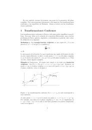
that the evolution of partisan conflict is remarkably similar to that of income inequality,proxied by the share of income held by the top 1%, in the postwar period. The increase ininequality observed since the late 1960s may be an important determinant of the rising trendin partisan conflict. This is consistent with McCarty, Poole, and Rosenthal (2003), who showthat partisanship became more stratified by income between 1956 and 1996. Prior to thisperiod, according to the authors, race and religion (rather than income and wealth) were thedominant determinants of political ideology.14030120GreatDepression25Partisan Conflict1008060‐ New Deal‐ D realignment‐ WWII201510Top one percent income share40Partisan ConflictTop 1% Share52018901893189618991902190519081911191419171920192319261929193219351938194119441947195019531956195919621965196819711974197719801983198619891992199519982001200420072010Year0Figure 5: Partisan conflict and income inequality, 1944-2012.Notes: Income inequality measured by the share of income held by the top 1%,from Alvaredo, Atkinson, Piketty, and Saez’s dataset. Data downloaded fromhttp://topincomes.parisschoolofeconomics.eu/.Causality, however, cannot be established, as argued by McCarty, Poole, and Rosenthal(2006). According to the authors, political disagreement can also affect income inequalityby hampering support for redistributive policies. This view is supported by the behaviorof partisan conflict and inequality in the late 1920s. Figure 5 shows that income inequalitypeaks right before the Great Depression, but exhibits a declining trend starting in 1929.Initially, inequality lowers due to the erosion of wealth in the top percentiles following thestock market crash. In addition, corporate taxes were raised and the top-bracket tax rate wasincreased from 25% to 63% under Hoover’s presidency. This resulted in further reductionsin the share of income held by the top 1%. From 1933 onwards, the size of the welfare statewas expanded to unprecedented levels in US history under the New Deal. Interestingly, thesenovel redistributive policies were approved in a period of unusually low levels of partisanconflict. PC scores were low for two reasons. First, polarization declined sharply duringthe 74th Congress (e.g., between 1935 to 1937) under Roosevelt’s presidency (see Figure 4).11
Ejemplo 60 El sistema{f k = 1 √2xe ikx }k∈Zes un sistema ortonormal completo en el espacio L 2 complejo ([−π, π]).Ejemplo 61 El sistema{d n (P n = c n · x 2dx n − 1 ) n, con cn = 1√ }2n + 1n! 2 n 2es un sistema ortonormal completo en L 2 ([a, b]) con la medida de Lebesgue. Aestos polonomios se les llama Polinomios de Legendre.Ejemplo 62 Tomemos L 2 (R, µ) con la medida∫µ (A) = h (x)dx,AA ∈ E con h (x) = e −x2 . Entonces el sistema { 1, x, x 2 , · · ·} es un sistemaortonormal completo en este espacio. Sin∈Ndn x2H n = c k edx n n ≥ 0, L ({H e−x2 0 , · · · , H n }) = L ({ 1, x, · · · , x 2n}) .A H n se les llama los Polinomios de Hermite.5 Funciones EspecialesExisten una serie de funciones que tienen caracteristicas muy particulares. Loimportante de estas funciones es que son solución de diferentes ecuaciones diferencialesmuy comunes en física, química, ingeniería, etc., por eso su estudiorequiere de una sección aparte. Hay una forma de estudiar todas estas funcionesespeciales de una forma unificada, es la versión que adoptaremos aqui.Todas estas funciones tienen caracteristicas comunes y adoptando esta versiónunificada es posible estudiar sus caracteristicas comunes de una sola vez.Definición 63 (Fórmula de Rodriques) Sead n1P n (x) = c nh dx n (hsn ), (1)tal que1) P n es un polinomio de grado n y c n una constante.2) s(x) es un polinomio de raices reales de grado menor o igual a 23) h : R → R es una función real, positiva e integrable en el intervalo[a, b] ⊂ R, (llamada peso) tal que h(a)s(a) = h(b)s(b) = 0.13