- Page 1:
ANÁLISIS NUMÉRICO SEGUNDA EDICIÓ
- Page 5 and 6:
Análisis numérico SEGUNOA EDICIÓ
- Page 7 and 8:
Contenido PREFACIO xüi CAPÍTULO 0
- Page 9 and 10:
Contenido | vil CAPÍTULO 4 Mínimo
- Page 11 and 12:
Contenido | ix 8.4 Ecuaciones difer
- Page 13:
Contenido | xi Apéndice B 590 B.1
- Page 16 and 17:
dv | Prefacio porque sabemos que el
- Page 18 and 19:
x v i | Prefacio Doron Levy Stanfor
- Page 21 and 22:
CAPITULO Fundamentos Este capitulo
- Page 23 and 24:
0.1 Evaluación de un polinomio | 3
- Page 25 and 26:
0.2 Números binarios | 5 0.1 Ejerc
- Page 27 and 28:
0 3 Números binarios | 7 0 .2 .2 D
- Page 29 and 30:
0 3 Representación del punto flota
- Page 31 and 32:
0 3 Representación del punto flota
- Page 33 and 34:
0 3 Representación del punto flota
- Page 35 and 36:
0 3 Representación del punto flota
- Page 37 and 38:
0.4 Pérdida de significancia | 17
- Page 39 and 40:
0.5 Repaso de cálculo | 19 0.4 Eje
- Page 41 and 42:
0.5 Repaso de cálculo | 21 // P j(
- Page 43 and 44:
Software y lecturas adicionales | 2
- Page 45 and 46:
1.1 B método de bisección | 25 1.
- Page 47 and 48:
1.1 B método de bisección | 27 co
- Page 49 and 50:
1.1 B método de bisección | 29 k
- Page 51 and 52:
U Iteración de punto fijo | 31 jet
- Page 53 and 54:
U Iteración de punto fijo | 33 En
- Page 55 and 56:
U Iteración de punto fijo | 35 y y
- Page 57 and 58:
U Iteración de punto fijo | 37 ►
- Page 59 and 60:
U Iteración de punto fijo | 39 ^ H
- Page 61 and 62:
U Iteración de punto fijo | 41 4.
- Page 63 and 64:
1 3 Límites de exactitud | 43 33.
- Page 65 and 66:
1 3 Límites de exactitud | 45 10 i
- Page 67 and 68:
1 3 Límites de exactitud | 47 enro
- Page 69 and 70:
1 3 Límites de exactitud | 49 La e
- Page 71 and 72:
1A Método de Newton | 51 1.3 Probl
- Page 73 and 74:
1A Método de Newton | 53 R g iira
- Page 75 and 76:
1.4 Método de Newton | 55 ftira es
- Page 77 and 78:
1.4 Método de Newton | 57 Se neces
- Page 79 and 80:
1A Método de Newton | 59 (a) xs -
- Page 81 and 82:
1 3 Localización de raíces sin de
- Page 83 and 84:
1.5 Localización de raíces sin de
- Page 85 and 86:
1.5 Localización de raíces sin de
- Page 87 and 88:
1.5 Localización de raíces sin de
- Page 89 and 90:
1.5 Localización de raíces sin de
- Page 91 and 92:
CAPITULO 2 Sistemas de ecuaciones L
- Page 93 and 94:
2.1 Eliminación gaussiana | 73 El
- Page 95 and 96:
2.1 Eliminación gaussiana | 75 El
- Page 97 and 98:
2.1 Eliminación gaussiana | 77 ANO
- Page 99 and 100:
2 J La factorización LU | 79 2.1 P
- Page 101 and 102:
2 J La factorizadón LU | 81 í\)r
- Page 103 and 104:
2 J La factorización LU | 83 Comen
- Page 105 and 106:
2 3 Fuentes de error | 85 4. Resuel
- Page 107 and 108:
2 3 Fuentes de error | 87 Al resolv
- Page 109 and 110:
2 3 Fuentes de error | 89 es ||A||
- Page 111 and 112:
2 3 Fuentes de error | 91 El factor
- Page 113 and 114:
2 3 Fuentes de error | 93 de donde
- Page 115 and 116:
2-4 La factorización PA = LU | 95
- Page 117 and 118:
2 A La factorizadón PA = LU | 97 2
- Page 119 and 120:
2-4 La factorización PA = LU | 99
- Page 121 and 122:
2A La factorización PA = LU | 101
- Page 123 and 124:
2A La factorización PA = LU | 103
- Page 125 and 126:
2A La factorización PA = LU | 105
- Page 127 and 128:
2 .5 Métodos iterativos | 107 Las
- Page 129 and 130:
2 .5 Métodos iterativos | 109 Obse
- Page 131 and 132:
2 .5 Métodos iterativos | 111 de l
- Page 133 and 134:
2 .5 Métodos iterativos | 113 2 .5
- Page 135 and 136:
2 .5 Métodos iterativos | 115 % Pr
- Page 137 and 138:
2 .6 Métodos para m atrices sim é
- Page 139 and 140:
2 .6 Métodos para m atrices sim é
- Page 141 and 142:
2 .6 Métodos para m atrices sim é
- Page 143 and 144:
2 .6 Métodos para m atrices sim é
- Page 145 and 146:
2 .6 Métodos para m atrices sim é
- Page 147 and 148:
2 .6 Métodos para m atrices sim é
- Page 149 and 150:
2 .6 Métodos para m atrices sim é
- Page 151 and 152:
2 .7 Sistem as de ecuaciones no lin
- Page 153 and 154:
2 .7 Sistem as de ecuaciones no lin
- Page 155 and 156:
2 .7 Sistem as de ecuaciones no lin
- Page 157 and 158:
2 .7 Sistem as de ecuaciones no lin
- Page 159 and 160:
3.1 Datos y funciones de interpolac
- Page 161 and 162:
3.1 Datos y funciones de interpolac
- Page 163 and 164:
3.1 Datos y funciones de interpolac
- Page 165 and 166:
3.1 Datos y funciones de interpolac
- Page 167 and 168:
3.1 Datos y funciones de interpolac
- Page 169 and 170:
3.1 Datos y funciones de interpolac
- Page 171 and 172:
3.2 Error de interpolación | 151 3
- Page 173 and 174:
3.2 Error de interpolación | 153 F
- Page 175 and 176:
3.2 Error de interpolación | 155 U
- Page 177 and 178:
3.2 Error de interpolación | 157 y
- Page 179 and 180:
3 3 Interpolación de C hebyshev |
- Page 181 and 182:
3 3 Interpolación de C hebyshev |
- Page 183 and 184:
3 3 Interpolación de C hebyshev |
- Page 185 and 186:
3 3 Interpolación de C hebyshev |
- Page 187 and 188:
3 .4 Splines cúbicas | 167 S,(x) =
- Page 189 and 190:
3 .4 Splines cúbicas | 169 ¿Cuán
- Page 191 and 192:
3 .4 Splines cúbicas | 171 Despué
- Page 193 and 194:
3 .4 Splines cúbicas | 173 y s = c
- Page 195 and 196:
3 .4 Splines cúbicas | 175 que se
- Page 197 and 198:
3 .4 Splines cúbicas | 177 9. Encu
- Page 199 and 200:
3.5 Curvas de Bézier | 179 15. Rec
- Page 201 and 202:
3.5 Curvas de Bézier | 181 un punt
- Page 203 and 204:
3.5 Curvas de Bézier | 183 3.5 P r
- Page 205 and 206:
3.5 Curvas de Bézier | 185 Figura
- Page 207 and 208:
Software y lecturas adicionales | 1
- Page 209 and 210:
4.1 Mínimos cuadrados y ecuaciones
- Page 211 and 212:
4.1 Mínimos cuadrados y ecuaciones
- Page 213 and 214:
4.1 Mínimos cuadrados y ecuaciones
- Page 215 and 216:
4.1 Mínimos cuadrados y ecuaciones
- Page 217 and 218:
4.1 Mínimos cuadrados y ecuaciones
- Page 219 and 220:
4.1 Mínimos cuadrados y ecuaciones
- Page 221 and 222:
4 .2 Exploración de m odelos | 201
- Page 223 and 224:
4 .2 Exploración de m odelos | 203
- Page 225 and 226:
4 .2 Exploración de m odelos | 205
- Page 227 and 228:
4 .2 Exploración de m odelos | 207
- Page 229 and 230:
4 .2 Exploración de m odelos | 209
- Page 231 and 232:
4 .2 Exploración de m odelos | 211
- Page 233 and 234:
4 3 Factorización QR | 213 '•i A
- Page 235 and 236:
4 3 Factorización QR | 215 m rn m
- Page 237 and 238:
4 3 Factorizadón QR | 217 El vecto
- Page 239 and 240:
4 3 Factorización QR | 219 ►EJEM
- Page 241 and 242:
4 3 Factorización QR | 221 Rgura4.
- Page 243 and 244:
4 3 Factorización QR | 223 EJEMPLO
- Page 245 and 246:
4 .4 Método del residuo mínimo ge
- Page 247 and 248:
4 A Método del residuo mínimo gen
- Page 249 and 250:
4 A Método del residuo mínimo gen
- Page 251 and 252:
4.5 Mínimos cuadrados no lineales
- Page 253 and 254:
4.5 Mínimos cuadrados no lineales
- Page 255 and 256:
4.5 Mínimos cuadrados no lineales
- Page 257 and 258:
4.5 Mínimos cuadrados no lineales
- Page 259 and 260:
4.5 Mínimos cuadrados no lineales
- Page 261 and 262:
4.5 Mínimos cuadrados no lineales
- Page 263 and 264:
C A P I T U L O 5 Diferenciación e
- Page 265 and 266:
5.1 Diferenciación numérica | 245
- Page 267 and 268:
5.1 Diferenciación numérica | 247
- Page 269 and 270:
5.1 Diferenciación numérica | 249
- Page 271 and 272:
5.1 Diferenciación numérica | 251
- Page 273 and 274:
5.1 Diferenciación numérica | 253
- Page 275 and 276:
5.2 Fórmulas de NewtonCotes para l
- Page 277 and 278:
5.2 Fórmulas de Newton-Cotes para
- Page 279 and 280:
5.2 Fórmulas de Newton-Cotes para
- Page 281 and 282:
5.2 Fórmulas de NewtonCotes para l
- Page 283 and 284:
5.2 Fórmulas de NewtonCotes para l
- Page 285 and 286:
5 3 Integración de Romberg | 265 2
- Page 287 and 288:
5 3 Integración de Romberg | 267 L
- Page 289 and 290:
5.4 Cuadratura adaptativa | 269 / \
- Page 291 and 292:
5.4 Cuadratura adaptativa | 271 La
- Page 293 and 294:
5.5 Cuadratura gaussiana | 273 3. R
- Page 295 and 296:
5.5 Cuadratura gaussiana | 275 Al a
- Page 297 and 298:
5.5 Cuadratura gaussiana | 277 1 .2
- Page 299 and 300:
5.5 Cuadratura gaussiana | 279 \ r
- Page 301 and 302:
CAPITULO Ecuaciones diferenciales o
- Page 303 and 304:
6.1 Problemas de valor inicial | 28
- Page 305 and 306:
6.1 Problemas de valor inicial | 28
- Page 307 and 308:
6.1 Problemas de valor inicial | 28
- Page 309 and 310:
6.1 Problemas de valor inicial | 28
- Page 311 and 312:
6.1 Problemas de valor inicial | 29
- Page 313 and 314:
6.2 Análisis del error en la soluc
- Page 315 and 316:
6.2 Análisis del error en la soluc
- Page 317 and 318:
6.2 Análisis del error en la soluc
- Page 319 and 320:
6 .2 Análisis del error en la solu
- Page 321 and 322:
6.2 Análisis del error en la soluc
- Page 323 and 324:
6 3 Sistema de ecuaciones diferenci
- Page 325 and 326:
6 3 Sistema de ecuaciones diferenci
- Page 327 and 328:
6 3 Sistema de ecuaciones diferenci
- Page 329 and 330:
6 3 Sistema de ecuaciones diferenci
- Page 331 and 332: 6 3 Sistema de ecuaciones diferenci
- Page 333 and 334: 6 3 Sistema de ecuaciones diferenci
- Page 335 and 336: 6 .4 Métodos y aplicaciones de Run
- Page 337 and 338: 6 .4 Métodos y aplicaciones de Run
- Page 339 and 340: 6 .4 Métodos y aplicaciones de Run
- Page 341 and 342: 6 .4 Métodos y aplicaciones de Run
- Page 343 and 344: 6 .4 Métodos y aplicaciones de Run
- Page 345 and 346: 6.5 Métodos con tamaño de paso va
- Page 347 and 348: 6.5 Métodos con tamaño de paso va
- Page 349 and 350: 6.5 Métodos con tamaño de paso va
- Page 351 and 352: 6.5 Métodos con tamaño de paso va
- Page 353 and 354: 6.6 Métodos implícitos y ecuacion
- Page 355 and 356: 6.6 Métodos implícitos y ecuacion
- Page 357 and 358: 6.7 Métodos de varios pasos | 337
- Page 359 and 360: 6.7 Métodos de varios pasos | 339
- Page 361 and 362: 6.7 Métodos de varios pasos | 341
- Page 363 and 364: 6.7 Métodos de varios pasos | 343
- Page 365 and 366: 6.7 Métodos de varios pasos | 345
- Page 367 and 368: Software y lecturas adicionales | 3
- Page 369 and 370: 7.1 Método de disparo | 349 7.1 M
- Page 371 and 372: 7.1 Método de disparo | 351 ginale
- Page 373 and 374: 7.1 Método de disparo | 353 Escrib
- Page 375 and 376: 7.1 Método de disparo | 355 2. Rea
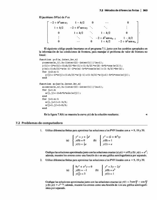
- Page 377 and 378: 7.2 Métodos de diferencias finitas
- Page 379 and 380: 7.2 Métodos de diferencias finitas
- Page 381: 7.2 Métodos de diferencias finitas
- Page 385 and 386: 7 3 Colocación y el método del el
- Page 387 and 388: 7 3 Colocación y el método del el
- Page 389 and 390: 7 3 Colocación y el método del el
- Page 391 and 392: 7 3 Colocación y el método del el
- Page 393 and 394: Software y lecturas adicionales | 3
- Page 395 and 396: 8.1 Ecuaciones parabólicas | 375 s
- Page 397 and 398: 8.1 Ecuaciones parabólicas | 377 i
- Page 399 and 400: 8.1 Ecuaciones parabólicas | 379 8
- Page 401 and 402: 8.1 Ecuaciones parabólicas | 381 c
- Page 403 and 404: 8.1 Ecuaciones parabólicas | 383 F
- Page 405 and 406: 8.1 Ecuaciones parabólicas | 385 F
- Page 407 and 408: 8.1 Ecuaciones parabólicas | 387 F
- Page 409 and 410: 8.1 Ecuaciones parabólicas | 389 u
- Page 411 and 412: 8.1 Ecuaciones parabólicas | 391 o
- Page 413 and 414: 8 .2 Ecuaciones hiperbólicas | 393
- Page 415 and 416: 8.2 Ecuaciones hiperbólicas | 395
- Page 417 and 418: 8.2 Ecuaciones hiperbólicas | 397
- Page 419 and 420: 8 3 Ecuaciones elípticas | 399 A s
- Page 421 and 422: 8 3 Ecuaciones elípticas | 401 A¡
- Page 423 and 424: 8 3 Ecuaciones elípticas | 403 «
- Page 425 and 426: 8 3 Ecuaciones elípticas | 405 Arg
- Page 427 and 428: 8 3 Ecuaciones elípticas | 407 Se
- Page 429 and 430: 8 3 Ecuaciones elípticas | 409 La
- Page 431 and 432: 8 3 Ecuaciones elípticas | 411 Rgu
- Page 433 and 434:
8 3 Ecuaciones elípticas | 413 A (
- Page 435 and 436:
8 3 Ecuaciones elípticas | 415 (a)
- Page 437 and 438:
IL4 Ecuaciones diferenciales parcia
- Page 439 and 440:
M Ecuaciones diferenciales parciale
- Page 441 and 442:
IL4 Ecuaciones diferenciales parcia
- Page 443 and 444:
IL4 Ecuaciones diferenciales parcia
- Page 445 and 446:
IL4 Ecuaciones diferenciales parcia
- Page 447 and 448:
IL4 Ecuaciones diferenciales parcia
- Page 449 and 450:
M Ecuaciones diferenciales parciale
- Page 451 and 452:
CAPÍTULO 9 Números aleatorios y s
- Page 453 and 454:
9.1 Números aleatorios | 433 x ¡
- Page 455 and 456:
9.1 Números aleatorios | 435 X Fig
- Page 457 and 458:
9.1 Números aleatorios | 437 aleat
- Page 459 and 460:
9.1 Números aleatorios | 439 La ve
- Page 461 and 462:
9.2 Simulación de Monte Cario | 44
- Page 463 and 464:
9.2 Simulación de Monte Cario | 44
- Page 465 and 466:
9.2 Simulación de Monte Cario | 44
- Page 467 and 468:
9 3 Movimiento browniano discreto y
- Page 469 and 470:
9 3 Movimiento browniano discreto y
- Page 471 and 472:
9 3 Movimiento browniano discreto y
- Page 473 and 474:
9A Ecuaciones diferenciales estocá
- Page 475 and 476:
9A Ecuaciones diferenciales estocá
- Page 477 and 478:
9A Ecuaciones diferenciales estocá
- Page 479 and 480:
9A Ecuaciones diferenciales estocá
- Page 481 and 482:
9A Ecuaciones diferenciales estocá
- Page 483 and 484:
9A Ecuaciones diferenciales estocá
- Page 485 and 486:
Software y lecturas adicionales | 4
- Page 487 and 488:
CAPITULO 10 Interpolación trigonom
- Page 489 and 490:
10.1 La transformada de Fourier | 4
- Page 491 and 492:
10.1 La transformada de Fourier | 4
- Page 493 and 494:
10.1 La transformada de Fourier | 4
- Page 495 and 496:
10.1 La transformada de Fourier | 4
- Page 497 and 498:
10.2 Interpolación trigonométrica
- Page 499 and 500:
10.2 Interpolación trigonométrica
- Page 501 and 502:
10.2 Interpolación trigonométrica
- Page 503 and 504:
1 0 3 FFT y el procesamiento de se
- Page 505 and 506:
1 0 3 FFT y el procesamiento de se
- Page 507 and 508:
1 0 3 FFT y el procesamiento de se
- Page 509 and 510:
1 0 3 FFT y el procesamiento de se
- Page 511 and 512:
1 0 3 FFT y el procesamiento de se
- Page 513 and 514:
1 0 3 FFT y el procesamiento de se
- Page 515 and 516:
CAPITULO 11 Compresión B movimient
- Page 517 and 518:
11.1 La transformada discreta del c
- Page 519 and 520:
11.1 La transformada discreta del c
- Page 521 and 522:
1 U TDC bidimensional y compresión
- Page 523 and 524:
1 U TDC bidimensional y compresión
- Page 525 and 526:
1 U TDC bidimensional y compresión
- Page 527 and 528:
1 1 3 TDC bidimensional y compresi
- Page 529 and 530:
1 U TDC bidimensional y compresión
- Page 531 and 532:
1 1 2 TDC bidimensional y compresi
- Page 533 and 534:
1 U TDC bidimensional y compresión
- Page 535 and 536:
1 1 3 Codificación de Huffman | 51
- Page 537 and 538:
1 1 3 Codificación de Huffman | 51
- Page 539 and 540:
11.4 TDC modificada y compresión d
- Page 541 and 542:
11.4 TDC modificada y compresión d
- Page 543 and 544:
11.4 TDC modificada y compresión d
- Page 545 and 546:
11.4 TDC modificada y compresión d
- Page 547 and 548:
11.4 TDC modificada y compresión d
- Page 549 and 550:
1 1 .4 TDC modificada y compresión
- Page 551 and 552:
CAPITULO 12 Valores y vectores cara
- Page 553 and 554:
12.1 Métodos de iteración de pote
- Page 555 and 556:
12.1 Métodos de iteración de pote
- Page 557 and 558:
12.1 Métodos de iteración de pote
- Page 559 and 560:
12.2 Algoritmo QR | 539 12.1 Proble
- Page 561 and 562:
12.2 Algoritmo QR | 541 que se llam
- Page 563 and 564:
12.2 Algoritmo QR | 543 Observe que
- Page 565 and 566:
12.2 Algoritmo QR | 545 es superior
- Page 567 and 568:
12.2 Algoritmo QR | 547 ► EJEM P
- Page 569 and 570:
12.2 Algoritmo QR | 549 4. 5. Repit
- Page 571 and 572:
12.2 Algoritmo QR | 551 donde p —
- Page 573 and 574:
1 2 3 Descomposición de valor sing
- Page 575 and 576:
1 2 3 Descomposición de valor sing
- Page 577 and 578:
12.4 Aplicaciones de la DVS | 557 3
- Page 579 and 580:
12.4 Aplicaciones de la DVS | 559 R
- Page 581 and 582:
12.4 Aplicaciones de la DVS | 561
- Page 583 and 584:
Software y lecturas adicionales | 5
- Page 585 and 586:
CAPITULO 13 Optimización B descu b
- Page 587 and 588:
13.1 Optimización no restringida s
- Page 589 and 590:
13.1 Optimización no restringida s
- Page 591 and 592:
13.1 Optimización no restringida s
- Page 593 and 594:
13.1 Optimización no restringida s
- Page 595 and 596:
13 .2 Optimización no restringida
- Page 597 and 598:
13.2 Optimización no restringida c
- Page 599 and 600:
13 .2 Optimización no restringida
- Page 601 and 602:
13.2 Optimización no restringida c
- Page 603 and 604:
Apéndice A: Álgebra matricial Se
- Page 605 and 606:
A.2 Multiplicación en bloque | 585
- Page 607 and 608:
L4 Matrices simétricas | 587 Las m
- Page 609 and 610:
A.5 Cálculo vectorial | 589 una fu
- Page 611 and 612:
B.2 Gráficas | 591 biarse con la i
- Page 613 and 614:
B 3 Programación en M a tla b | 59
- Page 615 and 616:
B.5 Funciones | 595 i f n2 (x) e x
- Page 617 and 618:
B.7 Animación y películas | 597 B
- Page 619 and 620:
Respuestas a los ejercicios selecci
- Page 621 and 622:
Respuestas a los ejercicios selecci
- Page 623 and 624:
Respuestas a los ejercicios selecci
- Page 625 and 626:
Respuestas a los ejercicios selecci
- Page 627 and 628:
Respuestas a los ejercicios selecci
- Page 629 and 630:
Respuestas a los ejercicios selecci
- Page 631 and 632:
Respuestas a los ejercicios selecci
- Page 633 and 634:
6.2 Ejercidos Respuestas a los ejer
- Page 635 and 636:
Respuestas a los ejercicios selecci
- Page 637 and 638:
Respuestas a los ejercicios selecci
- Page 639 and 640:
Respuestas a los ejercicios selecci
- Page 641 and 642:
Respuestas a los ejercicios selecci
- Page 643 and 644:
Respuestas a los ejercicios selecci
- Page 645 and 646:
Respuestas a los ejercicios selecci
- Page 647 and 648:
Bibliografía | 627 G. Birkhoff y G
- Page 649 and 650:
Bibliografía | 629 C. Edwards y D.
- Page 651 and 652:
Bibliografía | 6 31 M. Holmes [200
- Page 653 and 654:
Bibliografía | 633 J. A. Neldcr y
- Page 655 and 656:
Bibliografía | 635 J. C. Strikwerd
- Page 657 and 658:
índice actualización polinomio de
- Page 659 and 660:
Indice | 639 ecuaciones de Lorenz.
- Page 661 and 662:
Indice | 641 Mathematica. 23 Matlab
- Page 663 and 664:
índice | 643 mejorado, 298 orden,
- Page 665 and 666:
índice | 645 precondicionamiento,
- Page 668:
ANÁLISIS NUMÉRICO SEGUNDA EDICIÓ