université de montréal développement de la méthode sn à schémas ...

More documents

Recommendations

Info

112 I.2.2 Cas parabolique N subm 5 6 7 erreur relative ɛ max 0.01 0.005 0.0002 TAB. I.2 Erreur relative pour le cas parabolique etude de convergence: domaine monotonique 10 x 10−3 nombre de subdivision du maillage parabolique 9 8 7 erreur 6 5 4 3 2 5 5.2 5.4 5.6 5.8 6 6.2 6.4 6.6 6.8 7 FIG. I.4 Erreur relative pour le cas parabolique
113 −4.5 courbe log(e)=f(Nregions) cas parabolique −5 −5.5 log(erreur) −6 −6.5 −7 6.6 6.8 7 7.2 7.4 7.6 7.8 8 8.2 8.4 log(Nregions) FIG. I.5 Erreur relative pour le cas parabolique : courbe log-log Le coefficient directeur de la courbe de l’erreur en fonction du nombre de régions est d’environ M ≈ 1.6609.
Page 1 and 2:
UNIVERSITÉ DE MONTRÉAL DÉVELOPPE
Page 3 and 4:
À mes parents, Olivier et Anne Mar
Page 5 and 6:
vi RÉSUMÉ Le travail réalisé au
Page 7 and 8:
viii TABLE DES MATIÈRES DÉDICACE
Page 9 and 10:
x 2.3.2 Test de l’implémentation
Page 11 and 12:
xii CONCLUSION . . . . . . . . . .
Page 13 and 14:
xiv FIG. 3.10 FIG. 3.11 FIG. 3.12 F
Page 15 and 16:
xvi LISTE DES TABLEAUX TAB. 2.1 Ben
Page 17 and 18:
1 INTRODUCTION Le domaine de la sim
Page 19 and 20:
3 CHAPITRE 1 RÉSOLUTION DE L’ÉQ
Page 21 and 22:
5 - La variation du nombre de neutr
Page 23 and 24:
7 1.3 Traitement du terme de source
Page 25 and 26:
9 frontière est égal au flux sur
Page 27 and 28:
11 1.6.2 Quadratures angulaires pou
Page 29 and 30:
13 - Soient {i,j,k} les indices des
Page 31 and 32:
15 Z ez ξ Ω ψ (x,y,z) ω φ η e
Page 33 and 34:
17 Les termes {a,b,c} sont alors de
Page 35 and 36:
19 (Alcouffe, R.E. ; 1977), c’est
Page 37 and 38:
21 ̂Ω · −→ ∇δφ (κ+1/2)
Page 39 and 40:
23 Avec : P = I + D −1 E. (1.62)
Page 41 and 42:
25 On obtient ainsi une expression
Page 43 and 44:
27 FIG. 2.1 Système de coordonnée
Page 45 and 46:
29 u = 1 [ x − 1 ] ∆x i 2 (x i
Page 47 and 48:
31 Φ (α,∗,β) n,i,j,k±i/2 =
Page 49 and 50:
√ 5 ξ n ∆z k (Φ (1,0,∗) n,i
Page 51 and 52:
35 ordre M du schéma diamant class
Page 53 and 54:
37 - Cas parabolique (M=1) . La mat
Page 55 and 56:
39 φ n,i,j,k à partir de Q n,i,j,
Page 57 and 58:
41 nous avons comparé les résulta
Page 59 and 60:
43 Mélange Σ t Σ 0 s Σ 1 s νΣ
Page 61 and 62:
45 2.2.3.2 Test numéro 2 : Benchma
Page 63 and 64:
47 - Cas cubique : M=2. n Subm k ef
Page 65 and 66:
49 2.2.4.2 Test numéro 4 : géomé
Page 67 and 68:
51 le couplage entre les dérivés
Page 69 and 70:
53 des matrices d’assemblages (é
Page 71 and 72:
55 décroit très fortement avec le
Page 73 and 74:
57 - Cas cubique : M=2. n DSA Itér
Page 75 and 76:
59 Pour les deux premiers tests, le
Page 77 and 78: 61 6000 5500 5000 reduction du nomb
Page 79 and 80: 63 CHAPITRE 3 ÉTUDE DU BENCHMARK N
Page 81 and 82: 65 cartésiennes fixée comme origi
Page 83 and 84: 67 3.3 Valeurs recherchées Pour ch
Page 85 and 86: 69 - Ordre d’intégration spatial
Page 87 and 88: 71 3.4.2.1 Cas 222222 : Raffinement
Page 91 and 92: 75 On réalise maintenant la même
Page 95 and 96: 79 3.4.4 Étude de convergence pour
Page 99 and 100: 83 nimales de discrétisations angu
Page 101 and 102: 85 s’assurer que nos résultats n
Page 103 and 104: 87 3.5.2.1 Présentation des résul
Page 105 and 106: 89 erreur relative en % erreur rela
Page 107 and 108: 91 erreur relative en % erreur rela
Page 109 and 110: 93 Ces résultats peuvent être gé
Page 111 and 112: 95 120 100 Cas 111111 run3 80 60 40
Page 113 and 114: 97 Cas 311111 350 run3 300 250 erre
Page 115 and 116: 99 3.5.2.3 Analyse des résultats p
Page 117 and 118: 101 CONCLUSION Au cours de ce trava
Page 119 and 120: 103 RÉFÉRENCES Adams, M.L. & Lars
Page 121 and 122: 105 Expert group on 3D radiations t
Page 123 and 124: 107 Pour cela, on reprend le cas te
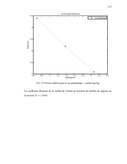
Page 125 and 126: 109 I.2 Étude du régime monotoniq
Page 127: 111 0 courbe log(e)=f(Nregions) cas
Page 131: 115 −5.8 −6 courbe log(e)=f(Nre
show all

université de montréal développement de la méthode sn à schémas ...

You also want an ePaper? Increase the reach of your titles

Delete template?

Save as template?