IV - Aérodynamique instationnaire des profils - Master 2 en ...
IV - Aérodynamique instationnaire des profils - Master 2 en ...
IV - Aérodynamique instationnaire des profils - Master 2 en ...

You also want an ePaper? Increase the reach of your titles
YUMPU automatically turns print PDFs into web optimized ePapers that Google loves.
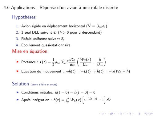
4.6 Applications : Réponse d’un avion à une rafale discrète<br />
Hypothèses<br />
1. Avion rigide <strong>en</strong> déplacem<strong>en</strong>t horizontal ( ⃗ V = U ∞ ⃗e x)<br />
2. 1 seul DLL suivant ⃗e z (h > 0 pour z <strong>des</strong>c<strong>en</strong>dant)<br />
3. Rafale uniforme suivant ⃗e z<br />
4. Ecoulem<strong>en</strong>t quasi-stationnaire<br />
Mise <strong>en</strong> équation<br />
◮ Portance : L(t) = 1 2 ρ∞U2 ∞S dC L<br />
dα<br />
(<br />
WG (x)<br />
U ∞<br />
+ ḣ<br />
U ∞<br />
)<br />
◮ Equation du mouvem<strong>en</strong>t : mḧ(t) = −L(t) ⇒ ḧ(t) = −λ(W G + ḣ)<br />
Solution (demo a faire <strong>en</strong> cours)<br />
◮ Conditions initiales: h(t = 0) = ḣ(t = 0) = 0<br />
◮ Aprés intégration : h(t) = ∫ t<br />
0 W G (x)<br />
[<br />
e −λ(t−x) − 1<br />
]<br />
dx