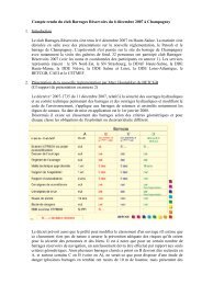
Laboratory experiments have been performed to study submarine and subaerial landslides (e.g., [3-7]),particularly in relation to case studies (see, [3] for a more detailed discussion of work to date), but these maybe both lengthy and costly to carry out. By contrast, numerical modeling, if properly validated withlaboratory experiments, may be a more flexible and efficient tool (e.g., [1], [6] and [9]). Moreover, numericalmodeling more easily provides flow variables for any point of space and, hence, is better suited to a detailedstudy of physical processes.Earlier modeling work of so-called tsunami landslides may be classified into two groups. In the first one,slide kinematics is a priori specified in the model, typically based on a semi-empirical equation, e.g.,describing the center of mass motion for solid landslides (e.g., [9-14]). This method has more often beenapplied to underwater landslides, for which induced free surface waves are usually initially less complex,although some authors have also applied it to subaerial landslides ([6],[15]). In the second group of methods,a fully coupled computation of both the slide and induced fluid motion is performed. Monaghan and Kos[16] thus use a Smooth Particle Hydrodynamics (SPH) method to study shallow water wave generation, dueto the impact of a falling rigid block. Panizzo and Dalrymple [17] also used a SPH model to studyunderwater landslide generated waves. Models based on a direct solution of Navier-Stokes (NS) equations,and featuring a free surface tracking algorithm, have also been used. Heinrich [18] and Assier Rzadkiewiczet al. [19] thus proposed two-dimensional (2D) NS simulations, with a Volume Of Fluids (VOF) type freesurface tracking, of both underwater and subaerial landslide tsunamis. Gisler et al. [20] recently proposed amodeling of the La Palma case study based on a compressible NS model, and Quecedo et al. [21] similarlymodeled the Lituya Bay case study with a multi-fluid NS model, in which both air and water motion weresimulated. These various NS model results are all quite promising, but the slide/fluid motion coupling stillneeds to be clarified, as it has not yet been fully studied. Also, a detailed analysis of physical processesinvolved has rarely been carried out.In this work, we present results of simulations of surface waves generated by subaerial landslides, obtainedwith the NS model Aquilon (developed in the Trefle laboratory, UMR 8508). In section 2, we brieflysummarize the equations and numerical methods for the model. In section 3, we present results of avalidation case for the 2D generation of a solitary wave by a falling block in shallow water. Finally, insection 4, the full potential of our model is illustrated by simulating the fully coupled case of wavesgenerated by a deformable slide moving down a slope.II NUMERICAL MODELThe computational domain is divided into three fluid subdomains: water, air and slide. In our approach, thelatter is also treated as a fluid, whose properties and constitutive law can be adjusted depending on watercontent and nature. Pierson and Costa [22] for instance indicate that, for water content greater than 50%,slides behave as Newtonian fluids. For smaller water contents, however, slides behave as viscoplastic fluids,with various constitutive laws depending on whether behaves more as a granular or a debris flow. The threefluids in the subdomains are similarly governed by incompressible NS equations:⎛ρ⎜∂U ⎝ ∂t∇ ⋅U = 0 (1)⎞+U⋅∇ ( )U ⎟ = ρg −∇P+∇( μ( ∇U +∇ t U)⎠(2)where U denotes the velocity vector and P the total pressure. The various fluids that co-exist in thecomputational domain are represented in Eq. (2) by their space-varying density ρ and viscosity μ. Equations(1) and (2) are discretized on a fixed structured grid, and solved using an augmented Lagrangian formulation[23]. The linear algebraic system obtained for each time step is solved using the iterative BiCGSTABalgorithm [24]. Since turbulence is not simulated in our model, results in fluid areas with strong shearstresses are to be taken with caution. Turbulence effects will be investigated in future work, which should bestraightforward considering that different turbulence models are already implemented in Aquilon.The motion of interfaces is represented by advection equations, expressed for a “volume fraction function”quantifying the fraction of each fluid present in interface cells, specifying that these interfaces are movingwith the flow. Here, two such equations can be expressed for the two interfaces between the three fluids :
C watertC slidetU C water 0 (3)U C slide 0 (4)where C water (resp. C slide ) is equal to 1 in water (resp. in the slide) and 0 everywhere else. Equations (3) and(4) are either solved using an explicit Total Variation Decreasing Lax Wendroff scheme of LeVeque [25]like in section IV, or with the PLIC-VOF reconstruction algorithm [26] like in section III. Lubin et al. [23]found that both methods lead to the same accuracy in the case of wave breaking simulation.Note, for interface cells, Eq. (2) is expressed using an equivalent density and viscosity, obtained by weighedaverage of individual fluid properties, based on their volume fraction in the cell. The whole model,composed of equations (1) to (4), is called a “one-fluid” model [27] because it approximates a three phaseflow with a single fluid formulation, in which the physical parameters are space varying. With such models,no conditions are required between the various fluid interfaces. The velocity continuity is implicitly specifiedin the model formulation itself.III VALIDATION CASEThe numerical model is first validated by simulating the 2D generation of a quasi-soliton in shallow water ofconstant depth, by a falling rigid block. This application, known as “Russel’s Scott wave generator”, hasbeen the object of well-controlled laboratory experiments as well as other numerical simulations. Figure 1shows the basic set-up and parameters for both the experiment and SPH simulations performed by Monaghanand Kos [16]. The experiment took place in a 2D flume, 9 m long and of variable depth D. A 38.2 kgrectangular block (0.4 m tall, 0.3 m long and 0.39 m wide; nearly the same as the inside of the flume) islocated just above still water level at initial time, and then released. Experiments were repeated for D =0.288, 0.210, and 0.116 m; in each case, the block vertical position and free surface elevation at a wavegauge located 1.2 m from the leftward extremity of the flume, were measured as a function of time.ywave gaugeD1.2 mxFigure 1 : sketch of Monaghan and Kos’ [15] experiment.Numerical simulations were performed using a 250x130 grid, with uneven cell dimensions in x (startingwith Δx min = 6 mm near the block and widening for larger x) and constant cell dimensions in y (Δ y= 6 mm).To closely reproduce experiments, in which the block was forced to have a vertical motion, horizontal blockvelocities are set to zero in the model. The block is represented by a very viscous fluid with μ = 10 4 Pa.s.Caltagirone and Vincent [28] have shown that, with such high viscosities, the local fluid flow within theblock behaves as a solid that only experiences a global translation or rotation (i.e. ∇×U = cst ). Slipboundary conditions are specified for the velocity components along all boundaries.Figure 2 shows numerical results at a few selected times, for D = 0.21 m. As in the experimental set-up,the block was slightly shifted rightward (by 25 mm), so that a very thin water sheet can rise to the left of itduring its fall, as can be seen on figure 2. Results show, as expected, that the numerical method allows theblock to keep its shape during motion, and hence to stay rigid. The main feature of the water flow is the
- Page 1 and 2:
Session 3Risques littoraux majeursP
- Page 4 and 5:
VI e Journées Scientifiques et Tec
- Page 6 and 7:
VI e Journées Scientifiques et Tec
- Page 8 and 9:
VI e Journées Scientifiques et Tec
- Page 10 and 11:
VI e Journées Scientifiques et Tec
- Page 12 and 13:
VI e Journées Scientifiques et Tec
- Page 14 and 15:
VI e Journées Scientifiques et Tec
- Page 16 and 17:
Colloque SHF "Valeurs rares et extr
- Page 18 and 19: Colloque SHF "Valeurs rares et extr
- Page 20 and 21: Hauteurs >ZH (cm)Saint-Jean-de-Luz2
- Page 22 and 23: Fréquence(%)3530252015Directions d
- Page 24 and 25: Fig. 4Station1. Saint-Jean-de-Luz2.
- Page 26 and 27: confrontés aux tendances passées
- Page 28 and 29: La majeure partie des indicateurs d
- Page 30 and 31: 1804 -4.8354 48.715 Au large de l
- Page 32 and 33: RUFINO DOS SANTOS T., PINOT J.-P.,
- Page 34 and 35: GoueltocGoulvenLe CurnicIle TariecR
- Page 36 and 37: 3203103002902802702602502401775 180
- Page 38 and 39: 7060504030201001775 1800 1825 1850
- Page 40 and 41: 315310305300Pt 1818295290285Pt 1804
- Page 42 and 43: MODELISATION DE L’IMPACT DU CHANG
- Page 44 and 45: évaluer leur importance lorsqu’i
- Page 46 and 47: l’enchaînement temporel des for
- Page 48 and 49: Morellato, D., Sabatier, F., Pon,s
- Page 50 and 51: CasHoule- intensité -Houle- durée
- Page 52 and 53: altitude m NGF (IGN 69)6543210-1-2-
- Page 54 and 55: 200augmentation de l'érosion (%180
- Page 56 and 57: Journées Scientifiques et Techniqu
- Page 58 and 59: Journées Scientifiques et Techniqu
- Page 60 and 61: Colloque SHF "Valeurs rares et extr
- Page 62 and 63: Colloque SHF "Valeurs rares et extr
- Page 64 and 65: Colloque SHF "Valeurs rares et extr
- Page 66 and 67: Colloque SHF "Valeurs rares et extr
- Page 70 and 71: development of a vortex at the bloc
- Page 72 and 73: moving slide among these three case
- Page 74 and 75: [3] Walder, J.S., P. Watts, O.E. So
- Page 76 and 77: Session 3 : Risques Littoraux Majeu
- Page 78 and 79: 6 ème journées scientifiques et t
- Page 80 and 81: 6 ème journées scientifiques et t
- Page 82 and 83: 6 ème journées scientifiques et t
- Page 84 and 85: 6 ème journées scientifiques et t
- Page 86: ABSTRACTObservations on the Impacts