Formulario - Sezione di Matematica - Sapienza

CORSO DI LAUREA IN INGEGNERIA EDILE - UNIVERSITÀ ”LA SAPIENZA”, ROMACORSO DI ANALISI MATEMATICA 2 (LETTERE M - Z) - a. a. 2007/’08FORMULARIO SINTETICO DI ANALISI MATEMATICA 2Coordinate polari{x = ρ cos(θ)y = ρ sin(θ), ρ ∈ [0, +∞) , θ ∈ [0, 2π)Coordinate polari centrate in P 0 ≡ (x 0 , y 0 ){x = x0 + ρ cos(θ)y = y 0 + ρ sin(θ), ρ ∈ [0, +∞) , θ ∈ [0, 2π)Coordinate ellittiche{x = aρ cos(θ)y = bρ sin(θ), ρ ∈ [0, +∞) , θ ∈ [0, 2π) , a, b > 0Coordinate ellittiche centrate in P 0 ≡ (x 0 , y 0 ){x = x0 + aρ cos(θ)y = y 0 + bρ sin(θ), ρ ∈ [0, +∞) , θ ∈ [0, 2π) , a, b > 0Differenziale totale e differenziabilitàSia f derivabile nel punto interno P 0 ≡ (x 0 , y 0 ).df(P 0 ) := f x (P 0 )(x − x 0 ) + f y (P 0 )(y − y 0 ) = f x (P 0 )dx + f y (P 0 )dy = −→ ∇f(P 0 ) · −→ dPf è differenziabile in P 0 ≡ (x 0 , y 0 ) sedove ρ = | −→ ∆P | =√(x − x0 ) 2 + (y − y 0 ) 2 .Formule di riduzione per gli integrali doppi∆f − df(P 0 )lim= 0ρ→0 ρSe T è un dominio normale rispetto all’asse x (o y-semplice):T = {(x, y) ∈ IR 2 | a ≤ x ≤ b ; α(x) ≤ y ≤ β(x)} , α, β ∈ C 0 ([a, b])∫∫Tf(x, y) dxdy =∫ bdx∫ β(x)a α(x)f(x, y)dy .Se T è un dominio normale rispetto all’asse y (o x-semplice):T = {(x, y) ∈ IR 2 | c ≤ y ≤ d ; γ(y) ≤ x ≤ δ(y)} , γ, δ ∈ C 0 ([c, d])1

∫∫Tf(x, y) dxdy =∫ ddy∫ δ(y)c γ(y)f(x, y)dx .Area di un dominio normaleSe T è un dominio normale rispetto all’asse x (o y-semplice):T = {(x, y) ∈ IR 2 | a ≤ x ≤ b ; α(x) ≤ y ≤ β(x)} , α, β ∈ C 0 ([a, b])Area(T ) =∫ ba[β(x) − α(x)]dx .Se T è un dominio normale rispetto all’asse y (o x-semplice):T = {(x, y) ∈ IR 2 | c ≤ y ≤ d ; γ(y) ≤ x ≤ δ(y)} , γ, δ ∈ C 0 ([c, d])Area(T ) =∫ dc[δ(y) − γ(y)]dy .Formule di trasformazione di coordinate nel pianoData la trasformazione invertibile di coordinate{ x = x(u, v)Φ :, Φ ∈ C 1 (A) , A ⊆ IR 2 , J(u, v) =y = y(u, v)∣ x uy u∣x v ∣∣∣≠ 0y vin A ,A = Φ(T ) , T = Φ −1 (A) ,cioè tale cheCoordinate polari:Φ −1 :{u = u(x, y)v = v(x, y)∫∫T{x = ρ cos(θ)y = ρ sin(θ)∫∫∫∫f(x, y) dxdy =T (x,y), J(x, y) =∣ u ∣x u y ∣∣∣ 1≠ 0 , J(x, y) =v x v y J(u, v) ,Af(x(u, v), y(u, v))|J(u, v)| dudv ., ρ ∈ (0, +∞) , θ ∈ [0, 2π) , J(ρ, θ) = ρ :∫∫f(x, y) dxdy =A(ρ,θ)f(x(ρ, θ), y(ρ, θ))ρ dρdθ .N.B.: in base a noti teoremi, la validità della formula di trasformazione in coordinate polaripuò essere estesa a (ρ, θ) ∈ [0, +∞) × [0, 2π].Volume di un dominio normale rispetto al piano (x, y)Dato il dominioT = {(x, y, z) ∈ IR 3 | (x, y) ∈ A ⊆ IR 2 , α(x, y) ≤ z ≤ β(x, y) , α, β ∈ C 0 (A)}2

∫∫V ol(T ) = [β(x, y) − α(x, y)] dxdy .AVolume di un solido di rotazioneDato il solido T ottenuto ruotando attorno all’asse z il rettangoloideR = {(x, z) ∈ IR 2 | z ∈ [c, d] , 0 ≤ x ≤ f(z)} ,detta x B l’ascissa del baricentro di R,V ol(T ) = 2π∫ ddz∫ f(z)x dx = π∫ dc 0c[f(z)] 2 dz = 2π · x B · Area(R)Formule di DirichletData f ∈ C 0 (D) , D ⊆ IR 2 ,Caso I. Funzione pari nella variabile x (f(x, y) = f(−x, y)) e dominio D simmetrico rispetto all’asse y:detto D 1 = D ∩ {(x, y) ∈ IR 2 | x ≥ 0}∫∫D∫∫f(x, y) dxdy = 2 f(x, y) dxdy .D 1Caso II. Funzione dispari nella variabile x (f(x, y) = −f(−x, y)) e dominio D simmetrico rispetto all’assey: ∫∫f(x, y) dxdy = 0 .DCaso III. Funzione pari nella variabile y (f(x, y) = f(x, −y)) e dominio D simmetrico rispetto all’asse x:detto D 2 = D ∩ {(x, y) ∈ IR 2 | y ≥ 0}∫∫D∫∫f(x, y) dxdy = 2 f(x, y) dxdy .D 2Caso IV. Funzione dispari nella variabile y (f(x, y) = −f(x, −y)) e dominio D simmetrico rispetto all’assex: ∫∫f(x, y) dxdy = 0 .DForme differenziali lineariω(x, y) = X(x, y)dx + Y (x, y)dyforma differenziale−→ F = (X(x, y), Y (x, y))campo vettoriale associato alla formaIntegrale curvilineo di forma differenzialeSe X , Y ∈ C 0 (A) , A ⊆ IR 2 connesso, data la curva regolare del pianoγ :{x = x(t)y = y(t), t ∈ [t 1 , t 2 ] , P (t 1 ) = P 1 , P (t 2 ) = P 23

allora∫ω :=γ(P 1 ,P 2 )∫ t2t 1[X(x(t), y(t)) · x ′ (t) + Y (x(t), y(t)) · y ′ (t)] dt .Metodi per il calcolo delle primitive V (x, y) di una forma differenziale esattaPrimo metodo: dato P 0 ≡ (x 0 , y 0 ) e il generico punto P ≡ (x, y) , P 0 , P ∈ A,V (x, y) =∫ x∫ yX(t, y 0 )dt + Y (x, t)dt + Cx 0 y 0oppureV (x, y) =∫ y∫ xY (x 0 , t)dt + X(t, y)dt + C .y 0 x 0Secondo metodo:oppure∫∫X(x, y)dx = V (x, y) + φ(y)dφdy = −∂V ∂y+ Y (x, y)Y (x, y)dy = V (x, y) + ψ(x)dψdx = −∂V ∂x+ X(x, y)Equazione della retta tangente a una curva regolare del piano nel punto di coordinate (x(t), y(t))y − y(t)y ′ (t)= x − x(t)x ′ (t)Componenti del versore tangente a una curva regolare del piano nel punto di coordinate(x(t), y(t))()vers( −→ x ′ (t)τ ) = √(x′ (t)) 2 + (y ′ (t)) , y ′ (t)√ .2 (x′ (t)) 2 + (y ′ (t)) 2Componenti del versore della normale interna a una curva regolare del piano nel punto dicoordinate (x(t), y(t))()vers( −→ y ′ (t)n i ) = −√ (x′ (t)) 2 + (y ′ (t)) , x ′ (t)√ .2 (x′ (t)) 2 + (y ′ (t)) 2Lunghezza di una curva regolareData la curva regolare del pianoγ :{x = x(t)y = y(t), t ∈ [t 1 , t 2 ] , P (t 1 ) = P 1 , P (t 2 ) = P 24

alloral(γ) =∫ t2t 1√(x′ (t)) 2 + (y ′ (t)) 2 dt .Se la curva γ è grafico della funzione y = f(x) , f ∈ C 1 ([a, b]), alloral(γ) =∫ ba√1 + (f′(x)) 2 dx .Equazione del piano tangente Π P0a una superficie regolare nel punto P 0 ≡ (x 0 , y 0 , z 0 )Data la superficie S grafico della funzione z = f(x, y) , f ∈ C 1 (A) , A ⊆ IR 2 , il piano tangente Π P0equazionez − z 0 = ∂f∂x (P 0) · (x − x 0 ) + ∂f∂y (P 0) · (y − y 0 )haComponenti del versore della normale interna alla superficie regolare nel punto P 0 ≡ (x 0 , y 0 , z 0 )()vers( −→ f x (P 0 )n i ) = √(fx (P 0 )) 2 + (f y (P 0 )) 2 + 1 , f y (P 0 )√(fx (P 0 )) 2 + (f y (P 0 )) 2 + 1 ,−1√(fx (P 0 )) 2 + (f y (P 0 )) 2 + 1Area della superficie∫∫Area(S) =A√(f x (x, y)) 2 + (f y (x, y)) 2 + 1 dxdyBaricentri e momenti di inerziaTutte le formule vanno intese per corpi aventi densità di massa uniforme e di massa unitaria.Coordinate del baricentro di un corpo γ filiforme nel piano, di equazioneγ :{x = x(t)y = y(t), t ∈ [t 1 , t 2 ] , P (t 1 ) = P 1 , P (t 2 ) = P 2x B = 1 ∫ t2x(t) √ (xl(γ)′ (t)) 2 + (y ′ (t)) 2 dt ; y B = 1 ∫ t2y(t) √ (xt 1l(γ)′ (t)) 2 + (y ′ (t)) 2 dt .t 1Coordinate del baricentro di un corpo D bidimensionale:x B =∫∫1Area(D) Dx dxdy ; y B =∫∫1Area(D) Dy dxdy .Coordinate del baricentro di un dominio T tridimensionale:x B =∫∫∫1V ol(T ) Tx dxdydz ; y B =∫∫∫1V ol(T ) Ty dxdydz ; z B =∫∫∫1V ol(T ) Tz dxdydz .Momento d’inerzia di un dominio T tridimensionale rispetto a un punto P 0 ≡ (x 0 , y 0 , z 0 ):5

∫∫∫I P0 =T∫∫∫[dist(P 0 , P )] 2 dxdydz =T[(x − x 0 ) 2 + (y − y 0 ) 2 + (z − z 0 ) 2 ] dxdydz .Momento d’inerzia di un dominio T tridimensionale rispetto all’asse delle z (analogamente per i momentid’inerzia rispetto agli altri due assi):∫∫∫I = (x 2 + y 2 ) dxdydz .TMomento d’inerzia di un dominio T tridimensionale rispetto al piano (x, y) (analogamente per i momentid’inerzia rispetto agli altri due piani coordinati):∫∫∫I = z 2 dxdydz .TDivergenza e rotoreDato il campo vettoriale −→ F = (X(x, y), Y (x, y)) ∈ C 1 (D) , D ⊆ IR 2 ,div( −→ F ) = −→ ∇ · −→ F := ∂X∂x + ∂Y∂y; rot( −→ F ) = −→ ∇ ∧ −→ F :=( ∂Y∂x − ∂X )−→k.∂yDato il campo vettoriale −→ F = (X(x, y, z), Y (x, y, z), Z(x, y, z)) ∈ C 1 (T ) , T ⊆ IR 3 ,div( −→ F ) = −→ ∇ · −→ F := ∂X∂x + ∂Y∂y + ∂Z∂z ;−→ −→ −→ i j k−−−−→rot( −→ F ) = −→ ∇ ∧ −→ F =∂∂∂∂x∂y∂z=∣ X(x, y, z) Y (x, y, z) Z(x, y, z) ∣=( ∂Z∂y − ∂Y ) (−→i ∂X+∂z ∂z − ∂Z ) (−→j ∂Y+∂x ∂x − ∂X )−→k∂yFormule di Gauss-Green in due dimensioni:Dato un dominio regolare e limitato D ⊂ IR 2 , considerate f, g ∈ C 1 (D),∫∫∫∫∂fD ∂x∫+∂Ddxdy = ∂gf dy ;D ∂y∫+∂Ddxdy = − g dx ;Applicazioni∫∫Area(D) = x dy = y dx = 1 ∫+∂D+∂D 2+∂D(x dy − y dx)Teorema della Divergenza in due dimensioni:∫∫div( −→ ∫∫ ( ∂XF )dxdy =DD ∂x + ∂Y ) ∫∫−→dxdy = (X dy − Y dx) = F · −→ ne ds∂y+∂D+∂D6

Teorema del Rotore (o di Stokes) in due dimensioni:∫∫D( ∂Y∂x − ∂X ) ∫dxdy = (X dx + Y dy)∂y+∂DTeorema del Rotore (o di Stokes) in tre dimensioni:Data una superficie S, grafico della funzione regolare z = f(x, y), definita su un dominio regolare D, fissatoarbitrariamente l’orientamento positivo del bordo +BS e orientati coerentemente S e il versore normalepositivo −→ n , considerato il campo vettoriale −→ F = (X(x, y, z), Y (x, y, z), Z(x, y, z)) ∈ C 1 (A) , S ⊂ A ⊆ IR 3 ,Φ S ( −−−−→rot( −→ ∫−−−−→F )) := rot( −→ ∫∮F ) · −→ −→n dS = X dx + Y dy + Z dz =: F · −→ τ dsS+BS+BSEquazioni differenziali a variabili separabilidydx = f(x) · g(y) ; f ∈ C0 (I x ) , g ∈ C 0 (I y ) .Metodo della separazione delle variabili: ponendo g(y) ≢ 0, si risolve∫∫dyg(y) =f(x)dxEventuali soluzioni singolari: si ottengono risolvendo g(y) = 0.(integrale generale)Equazioni differenziali lineari del primo ordine a coefficienti continuiy ′ (x) = a(x) · y(x) + b(x) ; a, b ∈ C 0 (I)∫Metodo del fattore integrante: e − a(x)dx∫∫e − a(x)dx [y ′ (x) − a(x) · y(x)] = e − a(x)dx b(x)∫d] ∫[e − a(x)dx y(x) = e − a(x)dx b(x)dxda cui∫ [∫a(x)dxy(x) = ee − ∫]a(x)dx b(x)dx + Covvero, usando la funzione integrale,∫ x[∫ x∫a(t)dtxy(x) = e 0 e − t]a(τ)dτx 0 b(t)dt + y0x 0, x 0 ∈ I ,dove, assegnato un Problema di Cauchy, y 0 = y(x 0 ).Equazioni differenziali di Bernoulliy ′ (x) = a(x) · y(x) + b(x) · y α (x) ; a, b ∈ C 0 (I) ; α ∈ IR , α ∉ {0, 1} .Solo se α > 0, occorre tener conto anche della soluzione singolare y ≡ 0.7

Supposto y ≢ 0, si pone z(x) = y 1−α (x), da cuiz ′ (x) = (1 − α)a(x)z(x) + (1 − α)b(x) .Equazioni differenziali lineari del secondo ordine a coefficienti costantiy ′′ (x) + ay ′ (x) + by(x) = f(x)y ′′ (x) + ay ′ (x) + by(x) = 0equazione non omogenea o completaequazione omogeneaIntegrale generale y 0 (x) dell’equazione omogenea: chiamiamo λ 1 e λ 2 le soluzioni dell’equazione caratteristica(o secolare)λ 2 + aλ + b = 0 .I caso (∆ > 0 , λ 1 , λ 2 ∈ IR , λ 1 ≠ λ 2 ) (radici reali e distinte):y 0 (x) = C 1 e λ1·x + C 2 e λ2·x , C 1 , C 2 ∈ IR .II caso (∆ = 0 , λ 1 = λ 2 = λ ∈ IR) (radici reali e coincidenti):y 0 (x) = C 1 e λ·x + C 2 · x · e λ·x , C 1 , C 2 ∈ IR .III caso (∆ < 0 , λ 1 = α + iβ , λ 2 = α − iβ = λ 1 ∈ IC) (radici complesse coniugate):y 0 (x) = e α·x [C 1 · cos(βx) + C 2 · sin(βx)] , C 1 , C 2 ∈ IR .Integrale generale y(x) dell’equazione non omogenea: detti y 0 (x) = C 1 y 1 (x) + C 2 y 2 (x) l’integrale generaledell’equazione omogenea associata e y(x) un integrale particolare dell’equazione non omogenea,y(x) = y 0 (x) + y(x)Metodo di Lagrange della variazione delle costantiy(x) = C 1 (x)y 1 (x) + C 2 (x)y 2 (x) ,doveC ′ 1(x)y 1 (x) + C ′ 2(x)y 2 (x) = 0ovverodove W (x) =∣ y 1(x)y 1(x)′⎧⎨⎩C 1(x)y ′ 1(x) ′ + C 2(x)y ′ 2(x) ′ = f(x)∫ f(x)y2 (x)C 1 (x) = −dx ; C 2 (x) =W (x)y 2 (x)y 2(x)′ ∣ è il Wronskiano di y 1 e y 2 .∫ f(x)y1 (x)W (x)dxMetodo di somiglianzaSi vedano anche le due pagine in fondo al formulario.8

1) f(x) = P m (x),con P m (x) polinomio di grado m in x:y(x) = p m (x) · x h ,dove h è la molteplicità (eventualmente nulla) della soluzione λ = 0 dell’equazione caratteristica e p m (x) èun generico polinomio di grado m in x.2) f(x) = e ηx P m (x),dove η ∈ IR , P m (x) polinomio di grado m in x:y(x) = e ηx q m (x) · x h ,dove h è la molteplicità (eventualmente nulla) della soluzione λ = η dell’equazione caratteristica e q m (x) èun generico polinomio di grado m in x.3) f(x) = e ηx [P m (x) cos(µx) + Q k (x) sin(µx)],dove η, µ ∈ IR , P m (x) , Q k (x) polinomi rispettivamente di grado m e k in x:y(x) = e ηx [p n (x) cos(µx) + q n (x) sin(µx)] · x h ,dove h è la molteplicità (eventualmente nulla) della soluzione λ = η + iµ dell’equazione caratteristica ep n (x), q m (x) sono generici polinomi di grado n = max{k, m} in x.Principio di sovrapposizioneData la generica equazione differenziale di ordine n lineare L(y) = f, con f = f 1 + f 2 , se esistono y 1 e y 2tali che L(y 1 ) = f 1 e L(y 2 ) = f 2 , allora la funzione y = y 1 + y 2 soddisfa l’equazione L(y) = f.9

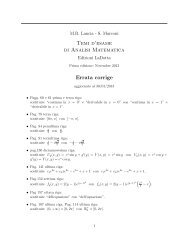
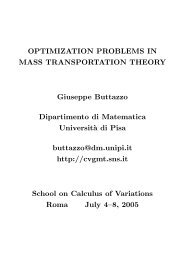
Punti critici liberi(da M. Bramanti, C.D. Pagani, S. Salsa, Matematica, Zanichelli, 2004)

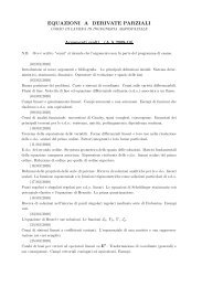
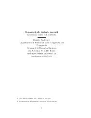
Metodo di somiglianza(da Krasnov, Kiselyov, Makarenko – A book of problems in ordinary differentialequations)