Optimality

260 G. Zheng, B. Freidlin and J. L. Gastwirth
Type I errors for all tests are expected to be close to the nominal level α = 0.05
and the powers of all tests are comparable. When HWE holds, the probabilities
(p0, p1, p2) for cases and (q0, q1, q2) for controls can be calculated using (3.1) under
the null and alternative hypotheses, where (g0, g1, g2) = (q 2 ,2pq, q 2 ) and (f1, f2) are
specified by the null or alternative hypotheses and D = � figi. After calculating
(p0, p1, p2) and (q0, q1, q2) under the null hypothesis, we first simulated the genotype
distributions (r0, r1, r2)∼mul(R; p0, p1, p2) and (s0, s1, s2)∼mul(S;q0, q1, q2) for
cases and controls, respectively (see Table 1). When HWE does not hold, we assumed
a mixture of two populations with two different allele frequencies p1 and p2.
Hence, we simulated two independent samples with different allele frequencies for
cases (and controls) and combined these two samples for cases (and for controls).
Thus, cases (controls) contain samples from a mixture of two populations with different
allele frequencies. When p is small, some counts can be zero. Therefore, we
added 1/2 to the count of each genotype in cases and controls in all simulations.
To obtain the critical values, a simulation under the null hypothesis was done
with 200,000 replicates. For each replicate, we calculated the test statistics. For each
test statistic, we used its empirical distribution function based on 200,000 replicates
to calculate the critical value for α = 0.05. The alternatives were chosen so that
the power of the optimal test Z0, Z 1/2, Z1 was near 80% for the recessive, additive,
dominant models, respectively. To determine the empirical power, 10,000 replicates
were simulated using multinomial distributions with the above probabilities.
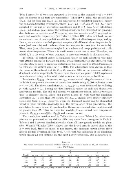
To calculate ZMERT, the correlation ρ0,1 was estimated using the simulated data.
In Table 3, we present the mean of correlation matrix using 10,000 replicates when
r = s = 250. The three correlations ρ 0,1/2, ρ0,1, ρ 1/2,1 were estimated by replacing
pi with ni/n, i = 0, 1,2 using the data simulated under the null and alternatives
and various models. The null and alternative hypotheses used in Table 3 were also
used to simulate critical values and powers (Table 4). Note that the minimum
correlation ρ0,1 is less than .50. Hence, the ZMAX3 should have greater efficiency
robustness than ZMERT. However, when the dominant model can be eliminated
based on prior scientific knowledge (e.g. the disease often skips generations), the
correlation between Z0 and Z 1/2 optimal for the recessive and additive models would
be greater than .75. Thus, for these two models, ZMERT should have comparable
power to ZMAX2 = max(|Z0|,|Z 1/2|) and is easier to use.
The correlation matrices used in Table 4 for r�= s and Table 5 for mixed samples
are not presented as they did not differ very much from those given in Table 3.
Tables 4 and 5 present simulation results where all three genetic models are plausible.
When HWE holds Table 4 shows that the Type I error is indeed close to the
α = 0.05 level. Since the model is not known, the minimum power across three
genetic models is written in bold type. A test with the maximum of the minimum
power among all test statistic has the most power robustness. Our comparison fo-
Table 3
The mean correlation matrices of three optimal test statistics based on 10,000 replicates
when HWE holds
p
.1 .3 .5
Model ρ 0,1/2 ρ0,1 ρ 1/2,1 ρ 0,1/2 ρ0,1 ρ 1/2,1 ρ 0,1/2 ρ0,1 ρ 1/2,1
null .97 .22 .45 .91 .31 .68 .82 .33 .82
rec .95 .34 .63 .89 .36 .74 .81 .37 .84
add .96 .23 .48 .89 .32 .71 .79 .33 .84
dom .97 .21 .44 .90 .29 .69 .79 .30 .83
The same models (rec,add,dom) are used in Table 4 when r = s = 250.