Underpinnings of fire management for biodiversity conservation in ...

Underpinnings of fire management for biodiversity conservation in reserves
Fire and adaptive management
Percent cover
64
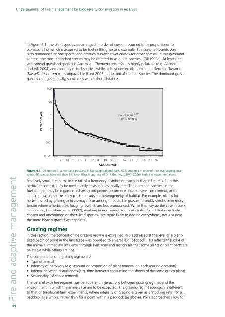
In Figure 4.1, the plant species are arranged in order of cover, presumed to be proportional to
biomass, all of which is assumed to be fuel in this grassland example. The curve represents very
high dominance of one species and drastically lower cover classes for other species. In this grassland
context, the most abundant species may be referred to as a ‘fuel species’ (Gill 1999a). At least one
widespread grassland species in Australia – Themeda australis – is highly palatable (e.g. Allcock
and Hik 2004) and a dominant fuel species; while at least one exotic dominant – Serrated Tussock
(Nassella trichotoma) – is unpalatable (Lunt 2005 p. 24), but also a fuel species. The dominant grass
species changes spatially, sometimes within short distances.
100
10
1
0.1
0.01
0.001
y = 72.406x -2.214
R 2 = 0.9866
1 7 13 19 25 31 37 43 49 55 61 67 73 79 85 91 97
Species rank
Figure 4.1 102 species of a montane grassland in Namadgi National Park, ACT, arranged in order of their overlapping cover
values; 95 species have less than 1% cover (Graph courtesy of Dr R Godfrey, CSIRO, 2006). Note the logarithmic Y-axis.
Relatively small rare herbs in the tail of a frequency distribution, such as that in Figure 4.1, in the
herbivore context, may be most readily envisaged as locally rare. The dominant species, in the
fuel context, may be regarded as having ubiquitous occurrence. In a conservation context, at the
landscape scale, species may persist because of heterogeneity of habitat. For example, niches for
herbs desired by grazing animals may occur among unpalatable grasses or prickly shrubs or in rocky
terrain where a herbivore’s foraging rewards are less pronounced. While this may be the case in some
landscapes, Landsberg et al. (2002), working in north-west South Australia, found that selectively
chosen and uncommon or short-lived species, ‘are more likely to decline everywhere’, not just near
the more heavily grazed water points.
Grazing regimes
In this section, the concept of the grazing regime is explained. It is addressed at the level of a plantsized
patch or point in the landscape – as opposed to an area e.g. paddock. This reflects the scale of
the animal’s immediate influence through herbivory and recognises that some plants or plant parts are
palatable while others are not.
The components of a grazing regime are:
• Type of animal
• Intensity of herbivory (e.g. amount or proportion of plant removal on each grazing occasion)
• Interval between disturbances (e.g. time between consuming the shoots of the same grassy plant)
• Seasonality (of shoot removal).
The parallel with fire regimes may be apparent. Interactions between grazing regimes and the
environment in which the animals live are to be expected. The grazing-regime approach is different
to that of traditional farm experiments, where intensity of grazing is given as a ‘stocking rate’ for a
paddock as a whole, rather than for a point within a paddock (as above). Point approaches allow for