Random Processes in Hyperbolic Spaces Hyperbolic Brownian ...
Random Processes in Hyperbolic Spaces Hyperbolic Brownian ...
Random Processes in Hyperbolic Spaces Hyperbolic Brownian ...

Create successful ePaper yourself
Turn your PDF publications into a flip-book with our unique Google optimized e-Paper software.
31 <strong>Hyperbolic</strong> <strong>Brownian</strong> Motion<br />
motion on H n may be obta<strong>in</strong>ed by solv<strong>in</strong>g the stochastic differential equations<br />
⎧<br />
⎨dXi(s)<br />
= Y (s)dBi(s), i = 1, ..., n − 1,<br />
⎩dY<br />
(s) = Y (s)dBn(s) − n−2Y<br />
(s)ds.<br />
By Itô’s formula we have that the solution {Z(t) = (X(t), Y (t)), t ≥ 0} satisfy<strong>in</strong>g Z(0) = z = (x, y)<br />
may be represented as follows:<br />
2<br />
⎧<br />
⎨Xi(t)<br />
= xi + y<br />
⎩<br />
t<br />
0 exp{Bµ (s)} dBi(s), i = 1, ..., n − 1,<br />
Y (t) = y exp{B µ (t)},<br />
where µ = (n − 1)/2 and B µ (t) = Bn(t) − µt has constant drift −µ. S<strong>in</strong>ce µ is assumed to be<br />
positive, Y (t) is the usual geometric <strong>Brownian</strong> motion with negative drift and then {Z(t), t ≥ 0}<br />
converges almost surely to the boundary of H n as t → ∞.<br />
3.2 <strong>Hyperbolic</strong> <strong>Brownian</strong> motion <strong>in</strong> H 2<br />
3.2.1 Transition function<br />
The 2-dimensional hyperbolic <strong>Brownian</strong> motion is a diffusion process on the upper half-plane<br />
H 2 = {z = (x, y) : x ∈ R, y > 0}<br />
associated with the Laplace operator ∆2 given by<br />
(3.7)<br />
∆2 = y 2<br />
2 ∂ ∂2<br />
+<br />
∂x2 ∂y2 <br />
. (3.8)<br />
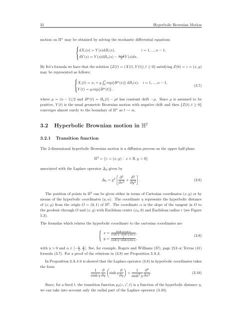
The position of po<strong>in</strong>ts <strong>in</strong> H 2 can be given either <strong>in</strong> terms of Cartesian coord<strong>in</strong>ates (x, y) or by<br />
means of the hyperbolic coord<strong>in</strong>ates (η, α). The coord<strong>in</strong>ate η represents the hyperbolic distance<br />
of (x, y) from the orig<strong>in</strong> O = (0, 1) of H 2 . The coord<strong>in</strong>ate α is the slope of the tangent <strong>in</strong> O to<br />
the geodesic through O and (x, y) with Euclidean center (x0, 0) and Euclidean radius r (see Figure<br />
5.3).<br />
The formulas which relates the hyperbolic coord<strong>in</strong>ate to the cartesian coord<strong>in</strong>ates are<br />
x =<br />
y =<br />
s<strong>in</strong>h η cos α<br />
cosh η−s<strong>in</strong>h η s<strong>in</strong> α ,<br />
1<br />
cosh η−s<strong>in</strong>h η s<strong>in</strong> α ,<br />
with η > 0 and α ∈ [− π π<br />
2 , 2 ]. See, for example, Rogers and Williams (37), page 213 or Terras (41)<br />
formula (3.7). For a proof of the relations <strong>in</strong> (3.9) see Proposition 3.A.3.<br />
In Proposition 3.A.4 it is showed that the Laplace operator (3.8) <strong>in</strong> hyperbolic coord<strong>in</strong>ates takes<br />
the form<br />
<br />
1 ∂<br />
s<strong>in</strong>h η<br />
s<strong>in</strong>h η ∂η<br />
∂<br />
<br />
1<br />
+<br />
∂η s<strong>in</strong>h 2 ∂<br />
η<br />
2<br />
.<br />
∂α2 (3.10)<br />
S<strong>in</strong>ce, for a fixed t, the transition function p2(z, z ′ , t) is a function of the hyperbolic distance η,<br />
we can take <strong>in</strong>to account only the radial part of the Laplace operator (3.10).<br />
(3.9)