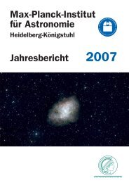
Max Planck Institute for Astronomy - Annual Report 2007

86 III. Selected Research Areas
sion is higher compared to the model with layered abundances.
The radial temperature gradient is also prominent
in this case.
The model without chemical stratification but with a
vertical temperature gradient also reveals the self-absorption
layer in the upper part of the channel map. The excitation
temperature of the HCO (4–3) transition changes
strongly with the disk height and has the lowest value
in the midplane. This zone of low intensity appears as a
fake “spiral arm” in the lower part of the map (marked as
“midplane” in Fig. III.3.5, middle panel). Note that such
a pattern somewhat resembles the “omega” structure for
the model with chemical stratification of HCO . While
only one representative channel is shown, one should
bear in mind that analysis of the interferometric data
is more reliable when all channels and dust continuum
emission are taken into account.
Despite the fact that all the models considered can
be distinguished in the synthetic channel maps, it is important
to study whether al m a is able to disentangle the
effects of thermal and chemical structure in disks. To
simulate the observations with al m a , use of the synthetic
HCO (4–3) channel maps is made as an input
to the gi l d a S simulation software. The focus lies on the
0.77 km s −1 channel (with 120 kHz bandwidth or 0.1 km
s −1 velocity width). Typical weather conditions at the
Chajnantor plateau are assumed, with the following main
types of errors leading to noise: 1) receiver temperature
is 80 K, system temperature is 230 K (at n 357 GHz,
see Guilloteau 2002), 2) random pointing errors during
the observation are 0.60, 3) relative amplitude errors are
3 % with a 6 % hour-1 drift, 4) residual phase noise after
calibration is 30°, 5) anomalous refraction. The object is
assumed to pass the meridian in the middle of a single
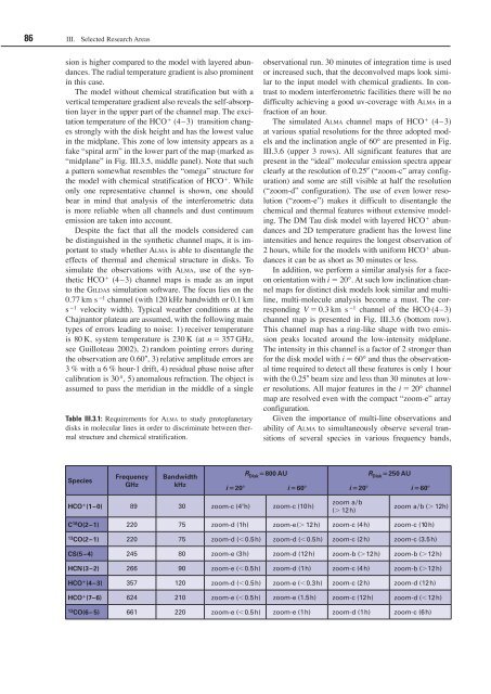
Table III.3.1: Requirements for al m a to study protoplanetary
disks in molecular lines in order to discriminate between thermal
structure and chemical stratification.
Species
Frequency
GHz
Bandwidth
kHz
HCO (1–0) 89 30 zoom-c (4h) zoom-c (10h)
observational run. 30 minutes of integration time is used
or increased such, that the deconvolved maps look similar
to the input model with chemical gradients. In contrast
to modern interferometric facilities there will be no
difficulty achieving a good uv-coverage with al m a in a
fraction of an hour.
The simulated al m a channel maps of HCO (4–3)
at various spatial resolutions for the three adopted models
and the inclination angle of 60° are presented in Fig.
III.3.6 (upper 3 rows). All significant features that are
present in the “ideal” molecular emission spectra appear
clearly at the resolution of 0.25 (“zoom-c” array configuration)
and some are still visible at half the resolution
(“zoom-d” configuration). The use of even lower resolution
(“zoom-e”) makes it difficult to disentangle the
chemical and thermal features without extensive modeling.
The DM Tau disk model with layered HCO abundances
and 2D temperature gradient has the lowest line
intensities and hence requires the longest observation of
2 hours, while for the models with uniform HCO abundances
it can be as short as 30 minutes or less.
In addition, we perform a similar analysis for a faceon
orientation with i 20°. At such low inclination channel
maps for distinct disk models look similar and multiline,
multi-molecule analysis become a must. The corresponding
V 0.3 km s −1 channel of the HCO (4–3)
channel map is presented in Fig. III.3.6 (bottom row).
This channel map has a ring-like shape with two emission
peaks located around the low-intensity midplane.
The intensity in this channel is a factor of 2 stronger than
for the disk model with i 60° and thus the observational
time required to detect all these features is only 1 hour
with the 0.25 beam size and less than 30 minutes at lower
resolutions. All major features in the i 20° channel
map are resolved even with the compact “zoom-e” array
configuration.
Given the importance of multi-line observations and
ability of al m a to simultaneously observe several transitions
of several species in various frequency bands,
R Disk 800 AU R Disk 250 AU
i 20 i 60 i 20 i 60
zoom a/b
( 12h)
zoom a/b ( 12h)
C 18 O(2–1) 220 75 zoom-d (1h) zoom-e( 12h) zoom-c (4h) zoom-c (10h)
13 CO(2–1) 220 75 zoom-d (0.5h) zoom-d (0.5h) zoom-c (2h) zoom-c (3.5h)
CS(5–4) 245 80 zoom-e (3h) zoom-d (12h) zoom-b (12h) zoom-b (12h)
HCN(3–2) 266 90 zoom-e (0.5h) zoom-d (1h) zoom-c (4h) zoom-b (12h)
HCO (4–3) 357 120 zoom-d (0.5h) zoom-e (0.3h) zoom-c (2h) zoom-d (12h)
HCO (7–6) 624 210 zoom-e (0.5h) zoom-e (1.5h) zoom-c (12h) zoom-d (12h)
13 CO(6– 5) 661 220 zoom-e (0.5h) zoom-e (1h) zoom-d (1h) zoom-c (6h)