popLA Manual (PDF) - Materials Science and Engineering

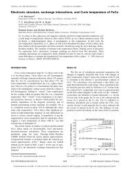
Figure 5 – DEMO_W-Q.DIF
Concerning Hardcopies
The prints you have been making are fast and adequate, but of lower resolution than the screen; and they do not
copy well. The figures in the document result from a different way of making hardcopies. We used a
commercial screen-dump program (GRAFLASR) to make a .PCX file, then opened it in PAINTBRUSH (within
WINDOWS 3.1), and printed in the "coarse-dither" option. To get all eight gray-shades, you must have a 256color
monitor. The figure may not look pretty to you now: but copy it (it works) and then copy it to a reduction
of less than 70%: it works, and it looks pretty. (If you want just a single figure, for example one transparency,
you can print out in high resolution with a 600dpi printer – but it doesn't copy well.)
Also try the regular Laserjet method (via F3), having loaded POPFONT?.HP when first entering POD).
This works as expected for 2 plots; for more plots, the arrangement on the hardcopy will be different from that
on the screen. The option to use PostScript is similar (via F4).
DISPLAY the three-dimensional Orientation Distributions (ODs)
Now inspect your .SOD (p.1#1). The format looks much like the .EPF, but there are only 19 lines of data in each
block. The OD (orientation distribution) files list the intensities in sections of 3-dimensional orientation space.
In the .SOD, each section is a “partial inverse pole figure”: partial in that the third angle is constant; the sum of
all sections is the projection, which is the inverse pole figure for axis 3, which is appended as the last block.
This file is only one way to arrange the derived densities in orientation space; it is the “Sample Orientation
Distribution”, or. SOD (with respect to crystal coordinates).
Each section contains one quadrant (for cubic crystal symmetry): 19 lines. The sections are given at every 5° of
the section angle. There are 19 of them (because we chose orthotropic sample symmetry). This is too many to
plot and inspect comfortably.
• Let us pare the file down to sections every 10°: p.5#5 will let you do this. Call the output file .SOS (the last S
for Selected sections). Plot it (p.6#2): 11 plots per page. If you use the scale 400/3 again, the last plot (the
projection) should look quantitatively like the .WIP plotted out before (only smaller in size). However, since
the densities in 3-D orientation space are usually higher than in the projections, it is better to plot it to a
different scale: try it now, using F2, (put a net on every plot for a change, but leave out the contours), then
choose the maximum 1600, next 3.
A different way to section orientation space is as "partial pole figures" or a "crystal orientation distribution", or
.COD (with respect to sample coordinates).
• To rearrange the OD that WIMV gave us from an .SOD to a .COD, use p.5#3, then again pare to something
you can plot: p.5#5, call .COS. Plot the 11 sections: the last one is the projection, which is the {001} pole
figure, and thus should be the same as the second plot on .WPF.
TUTORIAL 14