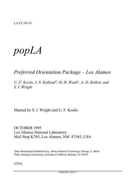
popLA Manual (PDF) - Materials Science and Engineering

LA-CC-89-18 

popLA 

Preferred Orientation Package – Los Alamos 

U. F. Kocks, J. S. Kallend*, H.-R. Wenk†, A. D. Rollett, and 

S. I. Wright 

Manual by S. I. Wright and U. F. Kocks 

OCTOBER 1995 

Los Alamos National Laboratory 

Mail Stop K765, Los Alamos, NM 87545, USA 

* Dept. Metallurgical & Materials Eng., Illinois Institute of Technology, Chicago, IL 60616 

† Dept. Geology & Geophysics, University of California, Berkeley, CA 94720 

GTDA 

INTRODUCTION 1

CONTENTS 

INTRODUCTION .........................................................................................5 

What does popLA do?.......................................................................................................................5 

Ownership .........................................................................................................................................5 

Problems............................................................................................................................................5 

Acknowledgments.............................................................................................................................5 

BASIC FEATURES.......................................................................................7 

Structure ............................................................................................................................................7 

Conventions.......................................................................................................................................7 

File Types and Names .......................................................................................................................7 

TUTORIAL....................................................................................................9 

BEFORE YOU START ....................................................................................................................9 

LOOK................................................................................................................................................9 

Plot......................................................................................................................................9 

Play .....................................................................................................................................9 

Print the plot......................................................................................................................10 

Inspect the file...................................................................................................................10 

MASSAGE......................................................................................................................................10 

Rotate................................................................................................................................11 

Smooth..............................................................................................................................11 

Normalize using the harmonic method..............................................................................11 

Analyze using the WIMV Method ......................................................................................12 

Concerning Hardcopies.....................................................................................................14 

DISPLAY the three-dimensional Orientation Distributions (ODs) .................................................14 

Discrete Grains Files.........................................................................................................20 

Weights .............................................................................................................................20 

DIOR.................................................................................................................................21 

DETAILS......................................................................................................22 

MAIN MENU (page 1) ...................................................................................................................22 

#1 Directory .....................................................................................................................22 

#2 Massage Data Files .....................................................................................................22 

#3 WIMV Analysis ..........................................................................................................22 

#4 Harmonic Analysis......................................................................................................22 

#5 Conversions.................................................................................................................23 

#6 Displays and Plots .......................................................................................................23 

#7 Properties ....................................................................................................................23 

#8 DOS ............................................................................................................................23 

MASSAGE (page 2)........................................................................................................................23 

#2 Create a Theoretical .DFB file ....................................................................................23 

#3 Digest Raw Data .........................................................................................................24 

#4 Rotate Pole Figures .....................................................................................................24 

#5 Tilt Pole Figures..........................................................................................................25 

#6 Symmetrize Pole Figures ............................................................................................25 

#7 Expand Pole Figures....................................................................................................25 

#8 Smooth Pole Figures ...................................................................................................25 

#9 Take Difference Between Two Pole Figures or ODs ..................................................26 

WIMV ANALYSIS (page 3) ..........................................................................................................26 

#2 Make SOD for High Symmetry Samples ....................................................................26 

#3 Make SOD for Lower Symmetry Sample ...................................................................27 

#4 Make SOD for Lower Symmetry Sample ...................................................................27 

INTRODUCTION 2

#5 Recalculate Pole Figures, High Symmetry..................................................................27 

#6 Recalculate Pole Figures, Low Symmetry ..................................................................27 

#7 Calculate Inverse Pole Figures from .SOD .................................................................27 

#8 Make WIMV Matrix ...................................................................................................27 

#9 Make WIMV Matrix for Inverse Pole Figures ............................................................27 

HARMONIC ANALYSIS (page 4) ................................................................................................28 

#2 Harmonic Analysis—Cubic ........................................................................................28 

#3 Harmonic Analysis—Lower Symmetry......................................................................28 

#4 Compute SOD.............................................................................................................29 

#5 Recalculate Pole Figures .............................................................................................29 

#6 Inverse Pole Figures....................................................................................................29 

#7 List Harmonic Coefficients .........................................................................................29 

#8 Establish coefficients for a transformation..................................................................29 

#9 Apply a transformation to given coefficients ..............................................................29 

CONVERSIONS (page 5)...............................................................................................................29 

#2 Permute axes in .SOD .................................................................................................29 

#3 Make .COD from .SOD (or .CHD from .SHD) ..........................................................30 

#4 Make OBLIQUE sections from .SOD file ..................................................................30 

#5 Pare to Subset for Display...........................................................................................30 

#6 Convert Miller Indices to Euler Angles.......................................................................30 

#7 DIOR See the description in the TUTORIAL section................................................30 

DISPLAYS AND PLOTS (page 6).................................................................................................31 

#2 Program POD..............................................................................................................31 

#3 Many contour plots (OD sections) from density files (Wenk program) ......................33 

#4 Single contour plot from density file (Wenk program) ...............................................33 

#5 Single contour PF from density file (Kallend program) ..............................................33 

#6 PFs, points or contours (Tomé program).....................................................................33 

#7 DIOR all OD sections and projections, compatible with POD....................................33 

#8 Square sections on the screen......................................................................................33 

#9 Square sections on the printer .....................................................................................33 

PROPERTIES (page 7) ...................................................................................................................34 

#2 Assign Weights To Discrete Grains File .....................................................................34 

#3 Elastic Properties.........................................................................................................34 

#4 Simulation of Polycrystal Plasticity ............................................................................34 

#5 Yield Locus Section ....................................................................................................35 

#6 Lankford Coefficients .................................................................................................35 

APPENDIX A – Computer Setup ..............................................................36 

A1 Hardware Requirements ...........................................................................................................36 

A2 Software Requirements.............................................................................................................36 

Memory and CONFIG.SYS..............................................................................................36 

Paths and AUTOEXEC.BAT............................................................................................36 

Screendump.......................................................................................................................37 

A3 Program Installation .................................................................................................................37 

A4 Some Features of DOS .............................................................................................................37 

APPENDIX B – popLA Conventions ........................................................38 

B1 File Extensions..........................................................................................................................38 

Pole Figure Files ...............................................................................................................38 

Analysis Input Files...........................................................................................................38 

WIMV Results Files..........................................................................................................38 

Harmonics Results Files....................................................................................................39 

Discrete Orientation Files .................................................................................................39 

Miscellaneous Files...........................................................................................................40 

B2 General Intensity File Format ...................................................................................................40 

B3 Conversion from other File Formats.........................................................................................41 

RAW data file format........................................................................................................41 

B4 Defocusing and Background Correction ...................................................................................43 

B5 Miller Indices Conventions.......................................................................................................43 

INTRODUCTION 3

B6 Format of Discrete Grains Files (TEXfiles, .WTS files)...........................................................44 

APPENDIX C – Sample Coordinate Systems ..........................................45 

The Euler Angle System (XYZ)......................................................................................................45 

The Sample Markings (123)............................................................................................................45 

The Goniometer System (ABN)......................................................................................................45 

The Plotting System (RTC).............................................................................................................45 

Summary and Recommendations ....................................................................................................45 

APPENDIX D – LApp DOCUMENTATION..........................................47 

D1 Introduction ..............................................................................................................................47 

D2 Installation................................................................................................................................47 

D3 Overview of Operation .............................................................................................................47 

Input Files .........................................................................................................................47 

Output Files.......................................................................................................................48 

Interactive Set-up ..............................................................................................................48 

D4 Details of File Formats .............................................................................................................50 

TEXIN ..............................................................................................................................50 

SXIN.................................................................................................................................51 

PROPIN ............................................................................................................................53 

BCIN.................................................................................................................................55 

TEXOUT ..........................................................................................................................55 

HIST .................................................................................................................................56 

ANAL ...............................................................................................................................57 

D5 Developments...........................................................................................................................58 

D6 LApp References......................................................................................................................58 

APPENDIX E – Custom Versions .............................................................60 

E1 I/O Redirection ..........................................................................................................................60 

E2 Command Line Interface ..........................................................................................................60 

UNRAW (Digest Raw Pole Figure Data – p.2#3).............................................................60 

ROTATE (Rotate Pole Figures – p.2#4) ...........................................................................60 

BWIMV (Calculate a .SOD – p.3#3) ................................................................................61 

BSOD2PF (Recalculate Pole Figures from a .SOD – p.3#6) ............................................61 

SOD2INV (Calculate Inverse Pole Figures from a .SOD – p.3#7) ...................................61 

CUBAN2 (Cubic Harmonic Analysis – p.4#2) .................................................................61 

WEIGHTS (Assign Weights To Discrete Grains File – p.7#2).........................................61 

REFERENCES ............................................................................................62 

INTRODUCTION 4

INTRODUCTION 

What does popLA do? 

popLA is a set of computer programs that help analyze texture in materials. It is designed as a coherent 

package, but individual programs may be used separately. Compatibility with other packages is achieved 

through various conversion programs. popLA is primarily designed to evaluate pole figures generated by 4circle 

goniometer X-ray diffraction equipment but can also be used with pole figures generated from other 

sources (e.g. neutron diffraction). popLA’s data analysis programs correct pole figure data for background Xray 

counts, the drop in measured intensity which occurs at the edge of the sample due to geometric 

considerations, and sample misalignment. Two types of analysis, the harmonic method and the WIMV method, 

may be used to calculate the orientation distribution of the sample. Pole figures and orientation distribution 

determined by popLA may be displayed or printed on a variety of hardware. 

Included with popLA is the Los Alamos polycrystal plasticity (LApp) code which may be used to simulate 

the development of texture during plastic deformation and to predict its effects on material properties. A short 

documentation for LApp is included; however, LApp may not be easy to use for the non-expert. 

Ownership 

©Copyright 1989, The Regents of the University of California and John S. Kallend. Major parts of the software 

package were produced under U. S. Government contract (W-7405-ENG-36) by Los Alamos National 

Laboratory, which is operated by the University of California for the U. S. Department of Energy. 

The U. S. Government is licensed to use, reproduce and distribute this software. Permission is granted to 

the public to copy and use this software without charge, provided that this notice and the above statement of 

authorship are reproduced on all copies. 

Neither the Government nor the University nor John S. Kallend makes any warranty, express or implied, or 

assumes any liability or responsibility for the use of this software. 

Problems 

We consider it part of the cooperative agreement with you that you let us know of any bugs you discover (and 

perhaps fix). If you feel that you have a problem, and have read all the painfully compiled instructions (on the 

screen and in the printed material), please contact us and we will try to help: 

Fred Kocks: FAX (505) 665-2992, or e-mail to: ufk@rho.lanl.gov; or 

Stuart Wright: FAX (505) 667-5268, or e-mail to: stuw@lanl.gov 

Fax is preferred. 

This is not a commercial product: we do not expect it to work immediately in an environment other than 

that for which it was created, nor work flawlessly for all applications even within this environment. For some 

such uses, we give recommendations, generally at the beginning of source codes; for others, you may have to use 

your own imagination. If you are interested in extensions that are not now supplied (such as a VAX version, 

which however would not be updated), you may succeed in engaging: 

John Kallend: FAX (312) 567-8875, e-mail METMKALLEND@karl.iit.edu. 

He is also knowledgeable on experimental details. For low-symmetry materials the contact is: 

Rudy Wenk: FAX (510) 643-9980, e-mail wenk1@UCBCMSA.berkeley.edu. 

Due to the fact that popLA is still under development, this manual will most likely not be completely up to 

date. The main purpose of this document is to give you basic instruction for using popLA . We would greatly 

appreciate hearing about any significant errors or omissions. 

Acknowledgments 

We are grateful for contributions, at various stages during the writing of the manual, by T. R. Bieler, R. B. 

Calhoun, S. R. Chen, M. R. Martinez, C. T. Necker, and A. D. Rollett. 

INTRODUCTION 5

BASIC FEATURES 

Structure 

popLA is a menu oriented program; it has a Main Menu from which the user gets to the second layer of menus, 

(entitled pages in this document) which call the various programs that do the actual calculations. Each program 

returns control to an appropriate page after completion. Navigation through the menus is accomplished by 

typing the number of the desired option. DO NOT press Return after entering an option; execution begins as 

soon as the number is typed. When input is requested within a program it must be followed by the Return key. 

Often when a program requests input it will display a frequently used default value. Pressing the Return key by 

itself will accept the default value for that option. 

In this document, information that popLA displays on the screen is displayed in the following format: 

Please type a number from 0 to 8 --> 

Information that you enter in respond is typed in bold italics. 

Please type a number from 0 to 8 --> 1 

In the documentation, the word “type” will be used when popLA expects input without the Return key, and 

“enter” when it expects the information to be followed by the Return key. 

Conventions 

At the menu stages of the program, entering option “0” terminates the program and returns control to the DOS 

command shell. Entering option “1” returns the program to the top menu level. Within programs there is no 

standard method for exiting the routine cleanly without execution,. Execution of a program can be halted by 

typing Control-C. popLA will respond 

Terminate batch job? (Y/N) Y 

Typing “Y” will return control the DOS command shell. You can restart popLA in the normal manner. Typing 

"N" will go back to a page of popLA. 

File Types and Names 

popLA makes extensive use of disk files. In fact, each program is a separate file which is loaded as required, a 

process invisible to the user. However, in order to effectively use the program it is necessary to understand the 

different types of data files that it creates. The majority of files are in standard ASCII text format and can be 

viewed with a variety of DOS utilities. There are essentially two kinds of files used by popLA – data files and 

property files. A description of the different types of files is given in Appendix B. 

Data files contain the actual data measured on the X-Ray machine or generated by a computer program. 

Each data file contains texture information about a specific sample. Each mathematical transformation 

performed by popLA produces a new file, which shares the same filename as the original data file but with a 

different extension. (e.g. AL2O3.RAW, AL2O3.EPF, etc.) We call the part of the filename before the extension 

the "specimen name" (or "specname" - AL203 in the above example). It should be entered as a parameter when 

starting popLA. In this manual, ".EPF" (etc.) means "specname.EPF": you must enter the whole filename. 

Because popLA can perform many different mathematical operations, a single data file created by an X-Ray 

machine can easily generate ten or more related data files. You may be concerned about the amount of space 

taken up by the various data files created by a single sample. There is no need to keep them all, since popLA 

can always re-create the files from the original data. Generally the .EPF file is kept rather than the .RAW file. 

The .SOD file is the parent of all files following from the WIMV analysis. 

Property files contain information used by popLA to perform various mathematical transformations. A 

single property file may be useful for many different samples. Property files are kept in the main directory C:\X 

so that they can be found easily by all users. Your own data files are best kept in a separate directory. 

BASIC FEATURES 7

TUTORIAL 

This section gives a quick guide through a “standard procedure” for an easy case. It is assumed, for this 

exercise, that you already have an “experimental pole figure (.EPF)” file: with experimental corrections like 

defocusing and background already incorporated, and in the right format. Appendix B2 will discuss how you get 

raw data into an .EPF file. 

The specimen name for this case is “demo”. All the files you will generate are already contained in 

C:\X\DEMO. In addition, this subdirectory contains a file TRY.EPF which is identical to DEMO.EPF and should 

be used to regenerate a whole set of TRY.* files (without overwriting the DEMO.* files). 

The sequence in this tutorial does not follow the sequence in the popLA menu, but rather how you might 

end up using popLA routinely later. References to the different screens are made by page number, to the option 

on that page by #; e.g.: p.2#4, page 2 (in this case the Massage page) option number 4 (in this case the Rotate 

Pole Figures option). 

BEFORE YOU START 

• popLA must have been installed (from the yellow and blue disks, see Appendix A3) into C:\X on a PC (which 

requires about 4 MB) 

• Your AUTOEXEC.BAT file must have been augmented as suggested in AUTOEXEC.POP: put C:\X into the 

path (preferably early); and (after the path statement) add the line: APPEND C:\X /path:on. There are 

some problems with this recommendation; for other options, see Appendix A3. 

• The computer must have been configured to have at least 540 MB of free memory (for some programs); this is 

the last number given as an answer to CHKDSK. 

LOOK 

At every stage, you will want to see what has been accomplished. We will use two instruments: 

p.1#1: lists a file (which we'll do later); and 

p.6#2: plots it on the screen and allows you to make hardcopies. The quickest way to make hardcopies (although 

not WYSIWYG) is by downloading our special fonts (POPFONT?.HP) to an HP Laserjet II or better: do this 

now by entering popLA (from your work directory), opting for p.6#2, and answering 2 to the first question; it 

will take a while but during any future use, skip this step by answering 0 to the first question. 

Plot 

Play 

Now stay within POD and merely RETURN upon every question (which selects default values), until it asks: 

"Enter name of data file # 1": try.epf 

and then again RETURN until you see that the calculations are running. Pretty soon, you'll see a pretty picture. 

• Press F1 repeatedly to see different colors and gray-shades; some have eight values, some fourteen (plus black 

and white); however, the contour lines are drawn in at eight levels only, in either case. 

• Look at the scale bar: there are numbers that go, in a logarithmic scale, from the minimum to the maximum. 

To get a nicer scale, press F2; when it asks you for a maximum, answer 400 (for this file), and then 3 to the 

next question. To all other questions, RETURN to get the defaults. Eventually, you'll see a new picture. Note 

that there are no contour lines (that was a default choice); that the region just above and just below random 

density have the same shade; and that pure black and pure white (or pink) are used to show regions in which 

the density is beyond the limits you specified. 

(At this point, you should perhaps stop playing for now, and go on.) 

TUTORIAL 9

Figure 1 – DEMO.EPF 

Print the plot 

Now press F3: it will make a file copy (black/white and with lower resolution) which you will then be given an 

option to print (hopefully self-explanatory). If the print doesn't come out right, restart the printer (thereby 

deleting all downloaded fonts) and then download ours again. 

Inspect the file 

Get yourself to page 1 of the menu and select 1, then try.epf. You will see the general format. (Press p to print 

out the file.) It will be worth your while to study Appendix B2 some time to understand all aspects of the 

format. For now, we emphasize only a few things: 

• The first line contains, in its first eight characters, the “specimen name” (here “demo”). This specimen name 

will be used by some of the programs, with new extensions. (The rest of line 1 can be arbitrary comments – 

some of which may get overwritten later.) 

• The second line has first an identifier ("(111)" in this case). Page down a few times to see that this file in fact 

contains 3 pole figures, identified with their indices, and separated by a blank line (and a repeat of the title 

line). 

•Go back home. In line 2, the next number is 5.0 (the angular increment in the radial direction) and then 80.0: 

this is the tilt to which measurements were made. Plots are always made to the angle listed in this position. 

Note, however, that the file contains numbers right up to 90°: these come from a simple extrapolation 

procedure for the purpose of providing a preliminary normalization of the pole figures. 

• In line 2, the second number from the end is 100: it is a scaling factor (multiplied by 100); if any of the data 

values would exceed 9999, the whole file is multiplied with a factor, and this factor (×100) is shown in line 2. 

(It would be less than 100.) 

• Immediately preceding the 100 are 3 integers (" 2 1 3" in this case) which reflect your choice of axis 

nomenclature, in the sequence right-top-center on the figure. You will note that what you looked at before had 

a "2" on the right – reflecting our choice to call the rolling direction "1" and plot it on top. Exit by pressing X. 

NOTE: It is at this stage that you should edit your .EPF file, if you ever want to, because all the information in it 

is carried forward to all subsequent files! 

MASSAGE 

There are three common things that one may wish to do with experimental pole figures before proceeding with a 

detailed analysis: rotate them, smooth them, and normalize them better. (Other "massaging" items will be 

discussed in the DETAILS section.) 

TUTORIAL 10

Rotate 

Smooth 

The experimental pole figures shown above seem to have some symmetry – except that it is not exactly aligned 

with the axes. This could, for example, be due to a slight misalignment of the specimen on the goniometer. If 

orthotropic symmetry were imposed on the data without first aligning them with the axes, some accuracy would 

be lost. 

• The program ROTATE (p.2#4, option 1) can analyze the data for this effect (by looking at sin terms in the 

harmonic expansion) and suggest an angle by which the pole figure should be rotated in order to make it as 

symmetrical as possible around the axes. In addition, you may wish to impose another rotation around the 

center of the pole figure; e.g., 90° if the way the specimen was mounted resulted in the rolling direction 

appearing on the right and you want it on top. 

(Other utilities in ROTATE are discussed in the DETAILS section.) 

The output file is called .RPF. 

Some data are very spotty; e.g., when only a few grains were covered. It is a matter of judgment in every case 

whether this effect should be smoothed out in the beginning, or at the end of the analysis (or never). 

• The program SMOOTH (p.2#8) provides an option to apply a Gaussian filter of arbitrary breadth to the data. 

We have found smoothing by 2.5° or 5° to be useful under some circumstances (remembering that this is 

about the grid resolution). You may try the program now using .RPF as an input. Note, however, that the 

“maximum” values observed in the texture decrease. For this reason, we will not use the smoothed file for 

further analysis, only perhaps for plotting. 

• The output file is called .MPF (“Massaged Pole Figure” – even when you later use it to smooth whole ODs). 

Inspect it via p.1#1: note that the two last actions were recorded on the title line. 

Normalize using the harmonic method 

The orientation distribution (OD) analysis in terms of spherical harmonics may be used as the principal tool of 

Quantitative Texture Analysis (QTA), or a discrete method may eventually be preferred by the user. Even in the 

latter case, harmonic analysis brings a significant initial advantage: it predicts the intensities in the unmeasured 

rim of all pole figures in a way that is consistent with all pole figures. In the process, all pole figures are renormalized, 

and this can be important (for example, in the WIMV program in popLA). 

• Use p.4#2, with your .RPF as input. Answer defaults, and use only the output file .FUL: it is identical to the 

input file except for the rim and the normalization. (The title line records this fact, but the two previous 

actions have now been dropped from being thus recorded.) 

This program is currently available only for crystal symmetries greater than orthorhombic and sample 

symmetries that have at least one two-fold axis in the center of the pole figure. 

Figure 2 – DEMO.FUL 

TUTORIAL 11

Analyze using the WIMV Method 

For this, you need the .FUL pole figures just obtained; WIMV will ignore the values above a tilt of 80° (but 

needs the normalization obtained in the last step). You also need "pointer files". They have the extension .WIM, 

.BWM, or .WM3, depending on which level of WIMV you use. Use the default files supplied for now. (Later 

you can make your own on p.4#8.) There are three levels of the WIMV program in popLA, depending on the 

complexity of your problem: look at p.4 numbers 2, 3, and 4. We have the easiest case, so we will use the fastest 

program: 

• Opt for p.4#2. Take the defaults on all options (especially the one on treating these as “incomplete” pole 

figures (even though they go to 90°). The progress will be displayed. The error estimates are listed for you 

to judge the rate of conversion. One may wish to stop when the change from one iteration to the next is only 

a fraction of a percent. (For the DEMO. files, we have stopped after iteration 17. The number of iterations, 

the final error estimate, and the Texture Strength will all be listed on the title line of the resulting .SOD and 

.WPF files. 

At the end you have an option as to which Euler angles you wish to have the files sequenced in. Your choice 

will be recorded in the output file, on the second line, position 5: B or R or K (for Bunge, Roe/Matthies, or 

Kocks). Pick 1 for now. 

• Before you look at the files, opt for p.4#7: make a file of WIMV-calculated inverse pole figures, .WIP. Since 

you have just made it, you may as well look at it first: 

• Opt for p.6#2 (for which you need to go back to p.1 first), answer 0, then defaults until "...plots on page?" If 

you answer 3, you get the whole file; but answer 2 to get the Z- and Y-axis pole figures. (You can print only 

2 plots in higher resolution). Note that a whole quadrant is shown even though, for this case, just one of the 

“stereographic triangles” would have been sufficient. (You can cut it out...) 

Figure 3 – DEMO.WIP 

• Now you are back on p.6, opt again for #2, etc., but this time look at .WPF: the WIMV-recalculated pole 

figures; the first two suffice. Use scale 400/3 again. Do they look familiar? They should be similar to the 

original .EPF, only rotated a bit and symmetrized, and completed in the rim. Since we assumed orthotropic 

sample symmetry (as one of the default answers while WIMVing), the four quadrants of the pole figure 

contain the same, averaged information. Plotting only one quadrant allows a better resolution of the figure in 

the same area. 

For a quantitative comparison of the recalculated and the input pole figures, we could either EXPAND the .WPF 

(p.2#7) or, which we suggest, SYMMETRIZE (p.2#6) the input pole figure. The actual input to WIMV was the 

.FUL pole figure, and we compare to it – firstly, because it has the rotation already built in, and second because 

it is properly normalized. As a fringe benefit, we get a comparison of the rim predictions from WIMV and from 

the harmonic method. Thus: 

TUTORIAL 12

• Opt for p.2#6 (via p.1), using .FUL as input, getting .QPF as output. Now back to p.6#2 (via p.1). Try 

something new: the third question within POD asks whether you want all standard options, and you have 

answered “yes” (0) so far. Answer 1 “for any change”. Now opt for the default of all options until the 

directive is “Enter the number of FILES to open”: answer 2. Now you know why it always asked 

you to “Enter the name of date file #1”. This will be the next question and you pick .QPF. For the 

“maximum” you pick 400, and for the next number enter 3. When the question data file #2 comes up, enter 

.WPF, then later the same scale options. You will get the {111} pole figures side by side (and to the same 

scale: one good reason to pick the scale yourself rather than taking the defaults!) Inspect the similarities and 

differences by eye. (You may also wish to get rid of the net in the right figure, or put a net on both: you can 

play using F2. But these nets don't print on the Laserjet by the procedure we are using now.) 

Figure 4 – DEMO.WPF and DEMO.QPF 

• To do the comparison between the two files in a quantitative way, opt for p.2#9 (via p.1) and make a 

difference file (.DIF), subtracting the .QPF from the .WPF. It will do it for all three pole figures. (It will ask 

you whether the difference in second-line parameters is OK: it is.) 

• Go to p.6#2 (you are already on p.6!), defaults, 2 plots, until it tells you “THIS FILE CONTAINS NEGATIVE 

INTENSITIES”: answer 2 to make a scale symmetric around zero. For the amplitude, pick 140. You will 

see, for both the {111} and {100} pole figures, the actual difference between recalculated and experimental 

values. Note that the differences are small everywhere but especially in the areas of very low density: this 

good fit is a consequence of the WIMV algorithm. It is also noteworthy that the peaks are higher 

(particularly, the "copper" and the "cube" orientations) than those predicted by the harmonic method. 

TUTORIAL 13

Figure 5 – DEMO_W-Q.DIF 

Concerning Hardcopies 

The prints you have been making are fast and adequate, but of lower resolution than the screen; and they do not 

copy well. The figures in the document result from a different way of making hardcopies. We used a 

commercial screen-dump program (GRAFLASR) to make a .PCX file, then opened it in PAINTBRUSH (within 

WINDOWS 3.1), and printed in the "coarse-dither" option. To get all eight gray-shades, you must have a 256color 

monitor. The figure may not look pretty to you now: but copy it (it works) and then copy it to a reduction 

of less than 70%: it works, and it looks pretty. (If you want just a single figure, for example one transparency, 

you can print out in high resolution with a 600dpi printer – but it doesn't copy well.) 

Also try the regular Laserjet method (via F3), having loaded POPFONT?.HP when first entering POD). 

This works as expected for 2 plots; for more plots, the arrangement on the hardcopy will be different from that 

on the screen. The option to use PostScript is similar (via F4). 

DISPLAY the three-dimensional Orientation Distributions (ODs) 

Now inspect your .SOD (p.1#1). The format looks much like the .EPF, but there are only 19 lines of data in each 

block. The OD (orientation distribution) files list the intensities in sections of 3-dimensional orientation space. 

In the .SOD, each section is a “partial inverse pole figure”: partial in that the third angle is constant; the sum of 

all sections is the projection, which is the inverse pole figure for axis 3, which is appended as the last block. 

This file is only one way to arrange the derived densities in orientation space; it is the “Sample Orientation 

Distribution”, or. SOD (with respect to crystal coordinates). 

Each section contains one quadrant (for cubic crystal symmetry): 19 lines. The sections are given at every 5° of 

the section angle. There are 19 of them (because we chose orthotropic sample symmetry). This is too many to 

plot and inspect comfortably. 

• Let us pare the file down to sections every 10°: p.5#5 will let you do this. Call the output file .SOS (the last S 

for Selected sections). Plot it (p.6#2): 11 plots per page. If you use the scale 400/3 again, the last plot (the 

projection) should look quantitatively like the .WIP plotted out before (only smaller in size). However, since 

the densities in 3-D orientation space are usually higher than in the projections, it is better to plot it to a 

different scale: try it now, using F2, (put a net on every plot for a change, but leave out the contours), then 

choose the maximum 1600, next 3. 

A different way to section orientation space is as "partial pole figures" or a "crystal orientation distribution", or 

.COD (with respect to sample coordinates). 

• To rearrange the OD that WIMV gave us from an .SOD to a .COD, use p.5#3, then again pare to something 

you can plot: p.5#5, call .COS. Plot the 11 sections: the last one is the projection, which is the {001} pole 

figure, and thus should be the same as the second plot on .WPF. 

TUTORIAL 14

• Now plot the .COD again, but in square sections. From within POD, opt for non-standard options: the first 

one is for ksquare. The best scale (which defaults to linear) is 700/0. The resulting plot is on a very coarse 

scale, but it should be recognizable to people who have worked with rolled FCC materials. 

. 

TUTORIAL 15 

Figure 6 – DEMO.SOS

. 

TUTORIAL 16 

Figure 7 – DEMO.COS

TUTORIAL 17 

Figure 8 – DEMO.COS Square sections

In all the polar figures, there is some concentration near the origin of many sections. (This is a cube component 

due to partial recrystallization.) In the square plot, the concentrations at the top line (at various places in the 

various sections) all correspond to this one component. The best way to avoid any degeneracies for this 

orientation is to use oblique sections. 

• Run p.5#4, take option 2, angles from 0 to 45°. The output is .CON. For the benefit of some improvement in 

the plots themselves, let us also smooth this file: go to p.2#8, range 5.0, do not treat as “INCOMPLETE pole 

figures”. The resulting file is called .MPF (and overwrote the smoothed .RPF you may have made early on. 

The best is to rename it to .CMN, which you can do by escaping to DOS (p.1#8), then type exit to come back 

to popLA. 

• Now plot (.MPF or .CMN): 10 sections. (The projection from this is the {001} pole figure again, but it is not 

plotted because, under some circumstances, the projections contains more, symmetrically equivalent 

components than are shown in the sections.) Scale 1600/3. 

• Try a few visual changes: F2, rewrite the first line to something descriptive, put a net on all plots, delete the 

Euler-angle information, stay with high resolution, but eliminate the contours (default!), finally change to 

vertical stacking (which allows you easier pasting for a “column figure”). 

TUTORIAL 18

. 

TUTORIAL 19 

Figure 9 – DEMO.CMN

Discrete Grains Files 

So far, we have described textures by densities in orientation space; even though they were assigned to discrete 

boxes, these were contiguous and meant to represent a continuous function. Under other circumstances, one 

describes textures by a set of discrete grains; for example, if they have been individually measured, or if they are 

the result of a simulation. One needs a way to convert one description into the other. 

Weights 

This program converts continuous distributions into discrete ones. As input, one needs a “grains” file that 

represents “no texture”. One can do this by picking a regular lattice of grains in orientation space or a random 

distribution. The grains are specified by a set of Euler angles. (The WEIGHTS program is written for one 

nomenclature only: the “symmetric” or “Kocks’” Euler angles). These grains will be assigned weights that 

reflect the density in orientation space at its location. We often assign different weights (near 1.0) to different 

grains even in the beginning: to make the random (or regular) distribution more isotropic. This can be tested by 

converting the grains files back to orientation distributions (see below: DIOR). 

• Try this for our example: p.7#2. For the initial grains file, use TEXCUB.WTS. This is a file that contains 

"triplets" of grains at positions that are equivalent due to the three-fold axis of the crystal symmetry. Use the 

triplets (256 of them, for a total of 768 orientations); the program will average the OD density at the three 

equivalent positions and deliver only the 256 irreducible orientations. 

• Another option you will have is to discard grains of low weight, such as to arrive at the smallest number of 

grains that describes your texture well enough. Try discarding all grains below a weight of 0.2. When the 

program is done, it will tell you how many grains are left, and what volume fraction was discarded (128, 0.05 

in our case). Now you must judge whether this is tolerable, or whether the number of grains is still too large; 

iterate until you are satisfied. The output file has the extension .WTS. 

• Inspect the resulting file (p.1#1). You see three columns of Euler angles and one of weights. (The weights 

are not necessarily normalized to 1.0: this must be done in subsequent programs.) The last line before the 

data block must contain, in its first position, the letter K (as it does here, for "Kocks" angles) or B or R or C. 

The first line, as always, contains the specimen name in its first 8 positions. The third line reflects the grain 

shape, which you have to edit yourself if you need it for future use (advanced topic). 

Figure 10 – DEMO.WTS 

TUTORIAL 20

DIOR 

This program goes the other way: the input is a (weighted) grains file, the output can be an orientation density 

file; other outputs are discrete plots and modified grains files. Before any output is produced, you may apply 

various symmetry operators, and decide how you want the data organized. Try it with the .WTS file produced 

above. 

• Go to DIOR (p.5#7). For the crystal symmetry file, enter cub.sym, for the sample symmetry file ort.sym. 

(It finds these in the c:\x directory; if it doesn't, say c:\x\cub.sym, etc.) Stay with the axes definition we 

picked originally: " 2 1 3" (this must be in 3i2 format -- you could permute the axes here). Opt to plot a 

pole figure (2). For the format of the plot, pick 2, for a single quadrant. Defaults 'til “intensity file” (1), "bin 

size" (5,5), defaults. Which pole figure? Pick 1,1,1 (later, 1,0,0). The output file is called DDEMO (a D 

prefixed to your specimen name). 

• Smooth it (p.2#8) by 2.5° (or 5° if you like). The output will be called DDEMO.MPF; go to DOS (p.1#8), 

rename DDEMO.MPF DEMOWTS.111. 

• Plot it (p.6#2), print it, compare to .WPF. 

• One more exercise. Use DIOR again, but this time ask for sample axes “ 1 3 2”, and plot the whole pole 

figure (plot style 0). You will see a rolling pole figure as if it had been taken from the transverse direction, 

with RD on the right, ND on top. 

Figure 11 – DEMOWTS.111 

TUTORIAL 21

DETAILS 

This section will detail page by page the menus used in popLA. Activate popLA by typing 

popla 

from anywhere. For the scientific background behind popLA refer to the paper entitled “Operational Texture 

Analysis” by J. S. Kallend, U. F. Kocks, A. D. Rollett and H.–R. Wenk published in Materials Science and 

Engineering, A132 (1991) pages 1-11. A corrected reprint is available and included with the package. 

MAIN MENU (page 1) 

You must return here to go from one page to another. 

popLA: preferred orientation package - Los Alamos (Page 1) 

J.S. Kallend, U.F. Kocks, A.D. Rollett, and H.R. Wenk (October 1993) 

0. QUIT 

1. Get specimen DIRECTORY and VIEW a file 

2. MASSAGE data files: correct, rotate, tilt, symmetrize, smooth, compare 

3. WIMV: make spec.SOD; calculate PFs and inverse PFs; make matrices 

4. HARMONIC analysis: COMPLETE rim (.FUL), get Roe Coeff.file (.HCF) 

5. CONVERSIONS, permutations, transformations, paring 

6. DISPLAYS and plots 

7. Derive PROPERTIES from .SOD or .HCF files, make WEIGHTS file for simul. 

8. DOS (temporary, type EXIT to return) 

Please enter a number from 0 to 8 --> 

#0 Quit 

This exits popLA and returns control to the DOS command shell. 

#1 Directory 

This option is to look at the contents of a data file within popLA. It displays all files name specname.* in the 

current directory and prompts 

Enter filename: 

The data file selected is passed to a program called LIST. LIST has many commands useful for looking through 

ASCII files. Type “P” to print what is displayed. It will continue printing upon Page Down – until “P” is 

toggled again. Type “X” to quit LIST and return to popLA. 

LIST is a shareware product with a $15 registration fee 

LIST Copyright 1986 by Vernon D. Buerg 

456 Lakeshire, Daly City CA 94015 

#2 Massage Data Files 

This option displays the Massage Data Files menu. This section of popLA is used for correcting raw data file 

obtained from X-Ray analysis for various effects and rotating the resulting pole figures so that the intrinsic 

sample symmetry is apparent. 

#3 WIMV Analysis 

WIMV analysis is the best method in popLA for determining orientation distributions. It is named for the 

authors of the algorithm—Williams, Imhof, Matthies, and Vinel. A short introduction to WIMV is given in a 

text by Wenk (1985) and a more detailed description in one by Matthies (1982). 

#4 Harmonic Analysis 

Another method of determining orientation distributions is harmonic analysis. An analytical solution to the 

orientation distribution function (ODF) is known for a special harmonic function. The coefficients of this 

function can be determined from the experimental data through an iterative process, allowing the ODF to be 

determined. The present harmonic analysis uses only the even (symmetrical) part of the ODF, which can lead to 

some errors in determining the true ODF. 

It is often useful to use harmonic analysis on a group of pole figures to extrapolate the pole figures to the very 

high tilt angles which cannot be measured experimentally, especially when there is significant intensity at the 

edge of the pole figure. After extrapolation the pole figure is re-normalized, giving more accurate intensities in 

the interior region, which can then be analyzed using WIMV. 

DETAILS 22

#5 Conversions 

There are a number of ways to represent the three dimensional orientation distribution in 2-D space. This section 

allows the sample SOD to be viewed displayed on different axes. It also contains DIOR , a program which can 

convert discrete grain files (those made up of a weighted set of Euler angles) from LApp to normal density files. 

#6 Displays and Plots 

This section of the program plots pole figures, inverse pole figures, and orientation distributions. Orientation 

distributions are fundamentally three dimensional in nature, so there are several different methods available for 

plotting the distribution in two dimensions. 

#7 Properties 

One of the most powerful features of popLA is the ability to predict the physical properties of materials and 

simulate the development of texture during deformation. The program which actually does this is known as 

LApp (Los Alamos Polycrystal Plasticity) which uses modifications of Taylor’s theory of polycrystalline 

plasticity to simulate the straining of materials. LApp requires that a texture be converted from an orientation 

distribution to a file which contains a finite number of grains of evenly spaced orientations, each “weighted” 

according to the texture of the material. LApp itself is complex and this document discusses only briefly in 

much detail how to use it. 

#8 DOS 

This allows the user to temporarily use DOS. To return to popLA, type EXIT from the same subdirectory popLA was 

started from. 

MASSAGE (page 2) 

MASSAGE DATA FILES (mostly PFs) (popLA page 2) 

0. Quit 

1. Return to Page 1 

2. Make THEORETICAL defocusing & background file: .DFB (R. Bolmaro) 

3. DIGEST Raw Data (.RAW), with defoc. & bkg (.DFB): make .EPF 

4. ROTATE PFs or adjust for grid offsets: make .RPF or .JWC 

5. TILT PFs around right axis (T. Ozturk) 

6. SYMMETRIZE PFs: make QPF or .SPF or .FPF 

7. EXPAND PFs back to full circle (needed for WIMV & harm.): .FPF 

8. SMOOTH PFs or ODs with Gaussian Filter (quad, semi, or full): make .MPF 

9. Take DIFFERENCE between 2 files (PFs or ODs): make .DIF 

Please enter a number from 0 to 9 ==> 

#0 Quit 

Selecting this option quits popLA and returns control to DOS command shell 

#1 Return to Page 1 

Selecting this option returns control to the main menu of popLA 

#2 Create a Theoretical .DFB file 

The .DFB (defocusing and background) file contains information necessary for popLA to correct for geometric 

defocusing and background X-Ray intensity. A unique .DFB file is required for each material, and, because the 

number of scattered X-Rays detected increases with the size of the detector slit, each slit width. .DFB files can 

be determined experimentally by running a sample with “random” texture on the X-Ray machine, to create a 

.COR file. Take the .COR file as input to COR2DFB (a program separate from popLA) to create .DFB file. 

Additional inputs to COR2DFB are the {hkl} of the pole figure correction data. 

Sometimes it is not convenient or even possible to create a .DFB file empirically. In this case it is possible 

to create a theoretical .DFB file which can be used instead. In order to create a theoretical .DFB, you must 

know the following information 

The detector slit width used 

The {hkl} of each measured pole figure 

The theta value of each {hkl} 

DETAILS 23

The width of each peak in degrees, the distance (in 2θ degree) between the point at which intensity 

decays to background level at the high side of the peak and corresponding point on the low side of the 

peak. 

This information can be obtained from a slow 2θ scan. When this option is selected popLA will prompt: 

Enter name of file : specname 

Enter only the filename; the .DFB extension will be added and the file stored in the default directory. (At Los 

Alamos, .DFB files are generally named in such a way that both the material and the slit width is incorporated 

into the file name, i.e. “TI3ALS40” for Ti3Al, slit width 4.0 mm.) When full pathnames are entered all but the 

first eight characters are truncated, generating unexpected results. The rest of the inputs are self-explanatory. 

Enter date, comments for the first line ( 1 

DETAILS 24

Select one of the options and enter the file name when requested. 

• Option 1: (most commonly used) popLA performs symmetry analysis on the sample and suggests a rotation 

angle which will improve sample symmetry. You may accept this angle or select your own. The output is an 

.RPF (rotated pole figure) data file. 

• Options 2 and 3: popLA changes the angular “phases”, e.g. from the 2.5°, 7.5°, . . . sequence (IW=0 or JW=0) to 

the 0°, 5°, . . . sequence. This is necessary if the programs are used as input to any of the analysis files 

(though not for the plotting programs, at least for POD). It should actually be done before the rotate step 

above. The output is a .JWC file. 

• Option 4: popLA inverts the spin of the sample. The output is a .-PF file. Note that this is not the same thing 

as an Inverse Pole Figure. The azimuthal spin in popLA data files is from the right to the top to left to the 

bottom and back. Some goniometers spin the other way and popLA assumes this as the norm: in going from 

.RAW to .EPF, the spin is inverted. To invert it back use Option 4. 

#5 Tilt Pole Figures 

This is similar to "Rotate", except that the rotation is performed about the horizontal axis in the pole figure. This 

option creates a .TPF (tilted pole figure) data file and returns control to the Massage Data menu. Upon 

selecting this routine the following is displayed: 

-TILT rotates pole figures around axis 

figure to be tilted, (default .WPF)? specname.ext 

-positive rotations move center up 

amount of rotation in deg.? 7 

If a rotation of 90° or greater is entered Tilt asks you whether you wish to record the permutation of the axes in 

the file. A rotation about the vertical axis can be achieved by first using Rotate to rotate the pole figure 90° 

about the axis normal to the page. Tilt can then be used to tilt the pole figure around the horizontal axis (the 

former vertical axis). This pole figure must then be rotated back 90° using Rotate to return to the original 

position. Tilt works only for complete pole figures, or for small tilt angles (since otherwise the area of lacking 

information in the rim is transferred into the central region). 

#6 Symmetrize Pole Figures 

An experimental data set is forced to conform to the presupposed sample symmetry. Symmetrize produces either 

a .QPF (quadrant pole figure) or a .SPF (semicircular pole figure) file depending on the selected sample 

symmetry. When this option is selected, popLA displays all data files in the present directory. Then: 

Input file (with .ext, default .RPF): 

Sample symmetry is: 

0. Orthorhombic 

1. Diad on Z 

Enter 0 or 1: 0 

If you want full (.FPF), say y or Y:n 

Some popLA operations (e.g., WIMV) require full, rather than half or quarter, pole figures. Entering “y” creates 

a full pole figure (.FPF). A .FPF file can also be created using the Expand Pole Figure option (4.2.7). Control is 

returned to the Massage Data menu. 

#7 Expand Pole Figures 

Some popLA options (e.g. WIMV) require full pole figures. This option creates full pole figures out of quarter 

or half pole figures using the intrinsic sample symmetry implied by these formats. When this option is selected, 

popLA displays 

(All .QPF and .SPF files in the present directory) 

Make a full pole figure from quadrant or semi 

Program by John Kallend 

Enter name of data file (with extension): specname.ext 

The output is a .FPF data file. Control is returned to the Massage Data menu. 

#8 Smooth Pole Figures 

This option applies a Gaussian filter to experimental derived pole figures in order to remove sharp spikes in the 

data which are uncharacteristic of real textures. Some loss of detail will occur. When this option is selected, 

popLA displays 

(All data files in the present directory) 

Gaussian smoothing of pole figure data 

Program by John Kallend (c) 1989 

Input file (with ext., default .EPF) specname.ext 

Smoothing range in degs. (w/dec pt.) --> 2.5 

DETAILS 25

The output is an .MPF file. Control is returned to the Massage Data menu. 

#9 Take Difference Between Two Pole Figures or ODs 

Sometimes it is helpful to take the difference between two pole figures or ODs, for example, in order to monitor 

textural evolution or to compare predictions with experiments. The program inspects the second line of both 

files for identity of the parameters. A warning is given if the two files do not appear to be similar enough for 

comparison – for example, a measured pole figure may say “(200)” and a calculated one “(001)”, in which case 

it is appropriate to compare the two pole figures and the warning should be ignored. The output of this option is 

a .DIF (difference) file. Control is returned to the Massage Data page menu. 

WIMV ANALYSIS (page 3) 

WIMV Analysis (popLA page 3) 

0. Quit 


WIMV: make .SOD and recalc pole figures .WPF -- for: 

2. cubic, tetra-, hexagonal crystals; sample diad; up to 3 PFs, 13 poles 

3. trigonal cry., gen’l.sample sym.,or higher: up to 7 PFs, 25 poles 

4. orthorhombic crystal; sample Z-diad: up to 7 PFs, 25 poles 

**or: orthorh,/gen’l/7/25 **requires 386, DOS 5, and 4MB memory ** 

Recalculate POLE FIGURES (even non-measured ones): make .APF- 

5. using .WIM matrix for the desired PFs (up to 3, 13 poles) 

6. using .BMW matrix for the desired PFs (up to 7, 25 poles) 

7. Calculate INVERSE pole figures from .SOD: .WIP 

8. Make WIMV matrix for new crystal structure and set of PFs: 

9. Make WIMV matrix for any INVERSE pole figures: make .WMI 


#0 Quit 

Quits program and returns control to DOS command shell 


Returns to the main menu of popLA 

#2 Make SOD for High Symmetry Samples 

This option determines the sample orientation distribution (SOD) for high symmetry samples using the WIMV 

algorithm. 

(Displays a list of .WIM files in C:\X\ directory) 

ODF ANALYSIS - WIMV ALGORITHM 

COPYRIGHT (C) 1987, 1988 JOHN S. KALLEND 

Enter the name of the wimv matrix (c:\x\?.wim) 

[Default is CUBIC] ==> 

You don’t have to enter the .WIM extension. If a .WIM matrix which corresponds to your sample symmetry 

does not exist, you will have to make one using option #7. 

Name of data file (default extension .EPF): 

You do have to enter the extension here. Using a .FUL file from harmonic analysis usually helps WIMV 

converge faster. 

Sample Symmetry is: 

0. Orthotropic 

1. Diad on Z 

Enter 0 or 1 ==> 0 

(Displays a list of pole figures in the data file) 

If you did use a .FUL data file for analysis, popLA displays 

Treat these as INCOMPLETE, OK? Y 

Press return for yes. popLA will then use only the data up to 80° of the pole figure, rather than the entire pole 

figure. Harmonic analysis helps to determine the intensities in the center more accurately but those extrapolated 

to high angles are not necessarily correct. popLA then displays information about the progress of the 

calculation, including the error of the ODF calculation and the texture "strength" (the root mean square density, 

i.e. the square root of the so-called "texture index"). 

DETAILS 26

After six iterations popLA asks if it should continue. Continue the iteration process until the error stops 

dropping rapidly. (Usually this is around 6 to 20 iterations.) An error of less than 5% is pretty good and 

indicates the pole figures used in the analysis are consistent with each other. 

Normalization factor: 0.95 

This is the correction factor that popLA had to apply in order for the average intensity of the data file to be 1.0. 

The closer to one, the less fudging WIMV had to do. 

In output file, angles increase from 0 in nomenclature of 

1. Kocks (need this one for WEIGHTS) 

2. Roe/Matthies 

3. Bunge (rotates plot +90 deg.) 

Enter 1,2, or 3 ==> 1 

Normally you should select 1 because the other options in popLA will all work if the SOD is described in Kocks 

nomenclature. For more information about Euler angles, see Kocks (1988). 

The output of WIMV analysis is a .SOD file, a density file which contains the orientation distribution with 

respect to the sample axes (longitudinal, transverse, etc.) in the requested format. Also produced is a .WPF file, 

which contains the same pole figures used in the analysis, recalculated from the SOD. Compare these with the 

original pole figures and make sure they are reasonable. Usually they look sharper than the originals. 

#3 Make SOD for Lower Symmetry Sample 

This is similar to #2 except for samples with low symmetry or higher pole multiplicity. 

#4 Make SOD for Lower Symmetry Sample 

This is similar to #3 but also incorporates orthorhombic crystal symmetry. This option is faster than #3 and 

requires a 386, DOS 5 and at least 4MB of memory. 

#5 Recalculate Pole Figures, High Symmetry 

Once the orientation distribution is known, the pole figure of any {hkl} in the crystal can be calculated, given the 

appropriate .WIM matrix (which can be created under p.3#8 below). This option creates an .APF (arbitrary pole 

figure) file. 

#6 Recalculate Pole Figures, Low Symmetry 

Similar to #5, but for crystals of low symmetry. A .BWM matrix is used instead of .WIM matrix. (It can also be 

created under p.3#8.) 

#7 Calculate Inverse Pole Figures from .SOD 

Another way of displaying texture data is to plot a particular sample orientation the framework of the crystal 

axes; this is called an inverse pole figure . It is especially useful for "fiber textures" in which only one sample 

axis special. This option of popLA creates inverse pole figures using the SOD determined by WIMV analysis. 

Output is a .WIP (WIMV inverse pole figure) file. 

#8 Make WIMV Matrix 

Before WIMV analysis can be performed on a sample, a WIMV matrix which contains information on the crystal 

symmetry must be created. WIMV matrices already exist for many materials but need to be created for others. 

There are three sub-options: to create 

• a .WIM matrix for use with p.3#2 

• a .BWM matrix for use with p.3#3 

• a .WM3 matrix for use with p.3#4 

#9 Make WIMV Matrix for Inverse Pole Figures 

This creates a WIMV matrix to project the .SOD onto an inverse pole figure for any sample direction. 

DETAILS 27

HARMONIC ANALYSIS (page 4) 

HARMONIC ANALYSIS (popLA page 4) 

0. Quit 


Find harmonic coefficients .HCF, completed PFs (.FUL) for: 

2. Cubic crystal system 

3. Hexagonal, tetragonal or orthorhombic crystal system 

4. Compute SOD or COD from harmonic coefficients (slow!) 

5. Recalculate pole figures .HPF 

6. Inverse pole figures .HIP 

7. List harmonic coefficients to screen or printer 

8. Establish coefficients for a given transformation 

9. Apply TRANSFORMATION to given coefficients 

Note: To convert Aachen-format Bunge coeffs. to Kallend’s binary 

Roe coeff.file .HCF: use AC2Wlmn (outside this menu) - 

Also need FAKTOR.CtW (J. Hirsch) 


#0 Quit 




#2 Harmonic Analysis—Cubic 

mn 

Determines the harmonic coefficients Wl from a sample with cubic symmetry--even l only, to l=22. When 

this option is selected, popLA displays 

Pole figure analysis to fit Wlmn, cubic 

Harmonic method 

Program (c) John Kallend 1971, 1982 

(x) Pole Figures read in 

How many iterations on missing parts? 6 

Six or eight iterations is usually sufficient. 

Sample Symmetry 


1. Mirror perpendicular to Z 

Enter 0 or 1 ==> 0 

After sample symmetry is entered, popLA determines the harmonic coefficients from the data. After the 

calculation is completed it will ask if you would like to print the harmonic coefficients to the screen. The output 

of this program is an .HCF file which contains the harmonic coefficients (in a binary format) and a .FUL file, 

which is a pole figure which has been extrapolated to low (non-measurable) angles using the harmonic 

coefficients determined during the analysis. Note that the .HCF file is not a density file like most of the files (i.e. 

pole figures) produced by popLA. 

#3 Harmonic Analysis—Lower Symmetry 

mn 

Determines the harmonic coefficients Wl (for l even, to 22) from a sample with orthorhombic, tetragonal, or 

hexagonal symmetry. It is necessary to know information about the unit cell because the sample is not cubic. 

The requests for input are self-explanatory. 

Pole figure analysis to fit Wlmn, non cubic 

Harmonic method 

Program (c) John Kallend 1971, 1982 

(x) Pole Figures read in 

How many iterations on missing parts? 6 

Six or eight iterations is usually sufficient. 

ODF Analysis for (file) 

Enter CRYSTAL SYSTEM code 

2=ORTHORHOMBIC, 4=TETRAGONAL, 6=HEXAGONAL 

Enter 2, 4, or 6 ===> 2 

(Program requests information about ratio of sides in the unit cell) 

Please enter sample symmetry: 

DETAILS 28


1. Mirror perpendicular to Z (monoclinic) 

After sample symmetry is entered, popLA determines the harmonic coefficients from the data. After the 

calculation is completed it will ask if you would like to print the harmonic coefficients to the screen. 

The output of this program is an .HCF file which contains the harmonic coefficients and a .FUL file, which 

is a pole figure which has been extrapolated to low (non-measurable) angles using the harmonic coefficients 

determined during the analysis. Note that the .HCF file is not a density file like most of the files (i.e. pole 

figures) produced by popLA. 

#4 Compute SOD 

The orientation distribution function for a sample can be calculated from the harmonic coefficients. It is usually 

less accurate than the WIMV method. Note that any negative density values (due to the assumption of l even 

only) are set to zero, and then the file is renormalized; this can lead to severe distortions. 

#5 Recalculate Pole Figures 

Once the harmonic coefficients (.HCF data file) are determined for a sample, any pole figure existing in the 

crystal system can be created. 

#6 Inverse Pole Figures 

This creates inverse pole figures from previously determined harmonic coefficients. 

#7 List Harmonic Coefficients 

This option lists the Roe harmonic coefficients. Control is returned to the harmonic analysis menu. 

#8 Establish coefficients for a transformation 

#9 Apply a transformation to given coefficients 

CONVERSIONS (page 5) 

CONVERSIONS of SODs, HCFs, and discrete angles files (popLA page 5) 

0. QUIT 

1. RETURN to Page 1 

--- ORIENTATION DENSITY FILES --- 

2. Permute axes in .SOD 

3. Make .COD from .SOD file (or .CHD from .SHD) 

4. Make OBLIQUE sections from .SOD files: .SON,.CON or .SHN,.CHN from .SHD 

(note: projections not reliable...) 

5. Pare to SUBSET for display: make .SOS or .COS (or .SHS, .CHS) 

--- DISCRETE ORIENTATION FILES --- 

6. Convert generic MILLER INDICES to any Euler angles 

7. DIOR: Add crystal symmetry and sample symmetries, permute axes, change 

angle convention, or make DENSITY file from DISCRETE grain file 


#0 Quit 




#2 Permute axes in .SOD 

We do not have a direct way to do this yet, but either of the following work: 

1) Use the .WPF file you already have 

(if it isn’t a full pole figure, first EXPAND: p2#7 to .FPF); 

ROTATE it (p2#4) 90 degs. around the center, or 

TILT it (p2#5) 90 degs. around the right axis 

(if you want to tilt around top axis, ROTATE 90 degs. before TILT); 

then re-run WIMV on the resulting .RPF or .TPF file. --- OR: 

2) Make a WEIGHTS file (p7#2), using a large number of grains. 

DETAILS 29

(However, if output >= 1152, you’d have to increase dimensions in DIOR.) 

Use DIOR (p5#7) with this file as input, and the symmetry files 

actually applicable to the SOD (e.g., cub.sym and ort.sym). 

Pick the axes permutation you want (need not be right-handed). 

Pick SOD, 19 quadrants to 90 deg. for cubic cry./ortho.sample, 

37 quadrants to 180 deg. for cubic cry./mono.sample, 

37 semis to 180 deg. for at least ortho./ortho. 

(lower symmetries won’t work this way). 

Ask for density file, 5 x 5 degs., defaults. 

Look at it (dspecnam): should have same format as original SOD, 

but with different IPER’s in line 2. Done. 

#3 Make .COD from .SOD (or .CHD from .SHD) 

This routine converts a sample orientation distribution into a crystal orientation distribution (regardless of how 

the SOD was obtained.) 

#4 Make OBLIQUE sections from .SOD file 

"Oblique sections" are handy to remove the last vestige of non-uniqueness at the origin; the sum (or difference) 

of the two azimuthal Euler angles is used as the section parameter. popLA does this only in the "symmetric" 

angle nomenclature, using the angle nu. 

The resulting file extension ends on N (.SON, .CON, etc.). The azimuth in the section may be chosen in an 

arbitrary manner; this distinguishes an .SON from a .CON. (A doubly oblique set is called an .OON.) 

In some versions, we append the projection, in some we do not. The reason is that one typically chooses as 

few sections as necessary, and then the sum of these sections is only part of the total projection. 

#5 Pare to Subset for Display 

Our displays typically accommodate only up to 12 figures. This option lets you pick an arbitrary selection of 

SOD sections (or COD section, CON sections, etc.) 

#6 Convert Miller Indices to Euler Angles 

The input is either one set of Miller indices (or direction indices) or a pair describing a full orientation (by one 

plane and one direction in it). For hexagonal crystals, the four-index notation is used. The program also needs a 

defined CRY.SYM in the directory (or the appended path) and will use this to calculate all symmetrically 

equivalent orientations for this crystal structure. The output file is called MILLER.EUL (overwriting any 

previous one!) and contains all these orientations in any of the Euler angle conventions we use (Bunge, Canova, 

Kocks, or Roe/Matthies). The format of this output file is that of a standard "weights file" or "discrete grains 

file". (Note that when the fourth column is left blank. the weight is assumed to be 1.0.) 

#7 DIOR See the description in the TUTORIAL section. 

The program DIOR (for DIscrete ORientations) was introduced in the tutorial for one purpose: to convert a 

discrete grains file into a density file (pole figure, inverse pole figure or any of the OD files). It also has plotting 

capabilities, which will be described under page 6,#7. 

Here we concentrate on its ability to manipulate an input weights file (DIORIN) and produce a new weights 

file (DIOROUT). One may increase the number of grains by adding all orientations that are symmetrically 

equivalent by virtue of any crystal symmetry elements or any sample symmetry elements. Conversely, one may 

reduce the number of grains by only keeping those within a certain part of orientation space (such as in one 

quadrant of a pole figure). The two actions often combine to leave the total number of grains constant (on 

purpose). In addition, one may change the Euler angle nomenclature, and one may permute the sample axes. 

(Note that, since both the input and the output are Euler angle files, the handedness must be kept the same; thus, 

if the input IPER was cyclic (e.g., the default 1 2 3), you must specify a cyclic output IPER (say, 2 3 1). 

When DIORIN and/or CRY.SYM and/or SAM.SYM exist in the subdirectory (or in the appended path), 

DIOR will take these and print some information that helps you recognize what was used. When they do not 

exist, DIOR asks you which file to use for DIORIN (e.g., MILLER.EUL), which for CRY.SYM (e.g., 

CUB.SYM -- which it will find in the appended C:\X), and which for SAM.SYM (e.g., ORT.SYM, ditto). 

To do these operations, DIOR has to reserve a certain amount of memory. We have different versions: the 

more recent ones use up to 540 KB of RAM (allowing up to 1002 input grains and 18 total symmetry operators). 

DIOR does not use extended memory. 

DETAILS 30

DISPLAYS AND PLOTS (page 6) 

DISPLAYS AND PLOTS (popLA page 6) 

0. Quit 


-------- POLAR REPRESENTATION (Wenk and Kocks) --------- 

DENSITY PLOTS: 

2. POD: colors or gray-shades on VGA 

(with possibility to capture into .PCX file or such) 

or (with less resolution) direct to hp-LASERJET or PS-file 

CONTOUR PLOTS: 

3. Many plots (OD sections) from density files (Wenk program) 

4. single PF from density file (Wenk program) 

5. single PF from density file (Kallend program, need PP.EXE or hp.plotter) 

DISCRETE ORIENTATION PLOTS: 

6. PFs, points or contours (Tome/Wenk program) 

7. DIOR: all OD sections and projections, compatible with POD 

-------- SQUARE SECTIONS (Kallend): cub/hex/tetr.cry.,ort/mono samples 

8. Colors on screen (fast, but limited options) 

9. Contours on hp-Laserjet (needs PP.EXE) or hp-plotter 


#0 Quit 

Selecting this option quits popLA and returns control to DOS command shell. 


Selecting this option returns control to the main menu of popLA. 

#2 Program POD 

This option displays "Polar Orientation Distributions" in up to 12 sections, or as pole figures or inverse pole 

figures. It requires input in the popLA format, with an angle registry that has the first value at zero (both 

radially and azimuthally). POD has many options, some refer to the hardware to be used, and others modify the 

appearance of the displays themselves. If you are a new user, selecting the defaults by pressing the Return key at 

the various options usually works. 

When the option is first selected, POD displays 

Do you wish to (first time around) 

1. Install program to PrintScreen to .PCX or .TIF file? (Need to restart) 

2. download POPFONTs for LaserjetII (or higher)? 

Enter one number or 0 for NO: ==> 2 

Selecting 2 loads a custom font into an HP Laserjet. (It works only for printers with the HP language.) This 

needs to be done each time the Laserjet is turned on. If you encounter trouble printing pole figures, turning the 

printer off and on again and reloading the custom fonts will sometimes help. 

0 Standard procedure (with options) 

1 Automatic quick scan of single patterns --> 0 

Option zero is normally used. Option 1 quickly displays a set of single pole figures, albeit at low resolution and 

with limited options. When Option 0 is selected, POD then displays 

THE DISPLAY SCHEME can be re-chosen later. 

Initial option: 

1 - 7 colors (+B+W) on black 

2 or 3 - 14 colors (+B+W) on black 

4 - 7 grey shades (+B,+W) on black 

5 - 7 grey shades (+B,+W), on white 

6 - 7 colors (+B) on white 

7 - LOW RESOLUTION (FAST, LO-RES, non-final, good for direct print) 

8 - NO DISPLAY, print equal area densities 

(interpolated on 36x36 grid) 

ID - - > 5 

DETAILS 31

5 is recommended for quick viewing of gray scale density plots. Pressing RETURN (or 0) activates the defaults 

specified in PODIN (see below). The next display reads: 

DEFAULT OPTIONS 

Input: 1 input file only 

output: interpolated (only if iw=jw=1) 

polar not square 

resolutions as chosen in PODIN lres 0 

contours as specified in PODIN: Y 

rotation as specified in PODIN : ang.= .0 

projection as specified in PODIN: kea = 1 

intensity scale as specified in PODIN 

(1:logarithmic, 2 linear) : klog 1 

(linear for difference file) 1 

Enter 0 for above standard, 1 for any changes -->0 

Answering 1 allows you to alter options for this particular run (and to plot 1 figure each from up to 3 files). The 

default (0) uses the values you specified (e.g., log or linear intensity scale) in the input file PODIN. One sample 

is provided in C:\X, but you may wish to have a different one on each subdirectory you use, for different 

applications. Just edit line 2 of PODIN according to the explanations provided right in the file. 

The size of each plot depends on how many are on page: 

on screen on laserjet 

quadrants or semis 1,2,3-6,7-12 1-2,3-11 (8) 

full circles 1,2, 3-12 1-2,3-11 

Enter the number of plots on page ( 1 

The above groups indicate the size of the plot. For example, selecting 3 on the LaserJet will print pole figures 

of the same size as if there were 11, which is quite small. 2 is the best for pole figures, and 10 for 5° spaced 

orientation distributions. 

You have to enter the of extension of the data file. 

Enter name of data file #1 -> filename 

0 to start with this data set 

n to skip n data sets --> 0 

You have to rerun POD for each page of output. This option lets you skip ahead to the pole figures you want to 

plot. For example, if you want to plot four pole figures, 2 per page, the first time through POD enter 0 here, and 

the second time enter 2 so that the pole figures you have already printed are skipped. 

POD then allows you to control the contours of the density plot. It displays 

Choose highest contour value 

0 

The default selects the maximum intensity appearing in the file. This give good results, but when comparing 

several pole figures it is helpful to keep the contours at the same level by explicitly specifying the top and bottom 

values. The numbers above are suggested top values (100 = random). 

-- How many shades below intensity 1.0 ? 

 

- -> 2 

In normalized data files, intensity 1 is "random", so this option allows you to determine the breakdown between 

the high and low intensity portions of the pole figure. The numbers above give scales if coupled with the top 

value in the same position on the previous questions. The default option allows you to specify the lowest 

intensity to be plotted instead of specifying the number of contours. If this is selected, POD will display 

Choose lowest contour value: 

-> 0 

Again, selecting the default will give good results, but sometimes it is desirable to specify a base value for 

consistency among different plots. 

POD now displays 

*** END OF INPUT SEQUENCE *** 

Then it beeps again and displays (sometimes). 

Do you wish to renormalize file? (1=yes) --> 0 

Normally press return for no. Otherwise POD will renormalize the data so that the average intensity is 1.0 and 

optionally write this to a .NPF file. POD then builds the plot in memory and displays it on the screen. 

The display now includes the texture "strength" if it was calculated in WIMV, in the top right corner. Below 

it is the "max" value of the actual density displayed (which is typically a little less than the maximum value on 

the file, because of interpolation). 

Once the entire screen is displayed, you may change the color or gray-shade scheme very rapidly by 

pressing F1. (ALT/F1 or CTL/F1 goes backwards.) The one that is actually displayed is dumped (see below). 

You may also change some of your previous options at this stage (even before the entire screen is 

displayed): press F2 and you may write a new title, add or delete contours, add or delete grids, re-scale, use a 

DETAILS 32

different resolution, toggle between equal-area and stereographic projections, and change the plot sequence to 

vertical or horizontal. Try it! 

The easiest method for direct printing is to hit the F3 key which will create the file POD?.HP (? increments 

from 1 through 9). Then you will be prompted for the POD?.HP files you wish to print. These files should be 

deleted after printing. Other useful output options are to create PostScript or PCX files. On the Los Alamos 

system the screen can be dumped to a Polaroid camera for slides or prints. Note that both the Laserjet and the 

PostScript files use a standard low resolution. The PCX files contain the exact information you see on the 

screen. Pressing F5 before dumping eliminates the control line. ESC leaves POD. 

CONTOUR PLOTS 

#3 Many contour plots (OD sections) from density files (Wenk program) 

This program does not work well on screen but produces very nice hp-Laserjet output (only very slowly indeed). 

The options are self-explanatory. Rudy Wenk uses this program to advantage for many PFs; for OD sections 

compatible with the rest of the package, we prefer POD prints (though it is more difficult to reproduce). 

#4 Single contour plot from density file (Wenk program) 

Similar to #3 above. 

#5 Single contour PF from density file (Kallend program) 

This is very fast, but low resolution. It first produces a plot file, which then must be converted to a Laserjet file 

by means of a program such as the commercial PrintAPlot (PP.EXE). 

DISCRETE ORIENTATION PLOTS 

#6 PFs, points or contours (Tomé program) 

This program requires special input files. It is no longer useful for point plots: use DIOR (#7); however, it is the 

only program producing contours directly from discrete grains files. An alternative is to use DIOR to make a 

density file and then plot this file using POD (for shades) or #4 or #5 above (for contours). 

#7 DIOR all OD sections and projections, compatible with POD 

This is the third time we have encountered the DIscrete ORientation program: this time to plot individual 

orientations. It is done with diamonds of an area proportional to the point weight. (Grains falling on the same 

point are integrated into a single weight.) The plot sizes, etc., are made identical to POD, so that one can 

produce a continuous and a discrete description of the same file to be overlaid (physically, with transparencies, 

or in a program such as PAINTBRUSH). 

Hardcopies can only be made via a screen dump: press F1 (or F5) first to invert black and white, then dump. 

"Dump" means: you must have loaded a screen dump program (such as GRAFLASR) before; then pressing Print 

Screen (while in graphics mode) will produce a .PCX file (or whatever you set up for). 

#8 Square sections on the screen 

This prints an orientation distribution in square sections on the screen. It is low resolution, not interpolated, and 

very fast: merely offered for a quick comparison. 

#9 Square sections on the printer 

This option makes contour plots of an orientation distribution on a plotter or an HP LaserJet via Laserplotter. It 

asks for the filename to print and the destination of the plot. 

DETAILS 33

PROPERTIES (page 7) 

Properties (popLA page 7) 

0. Quit 

1. Return to page one 

2. Assign Weights to discrete grains file from .SOD 

(Need Kocks style Euler angles in both .SOD and TEXfilecan 

convert the latter in DIOR, p.5,7) 

3. Average elastic properties (Reuss, Voigt, Hill, self-consistent) 

(Program by C. Tome) Input ELTEX.DAT, ELMOD.DAT; out ELOUT?.DAT 

4. Simulation of polycrystal plasticity from weighted grain file - 

LApp code: with rate sensitivity and grain shape effects, 

for all crystal and sample symmetries, 

calculate current yield surface, Lankford coefficients; 

predict texture development, Taylor factors, 

stress/strain curves for all straining paths. 

SHEET properties directly from harmonic coefficients 

(orthotropic plane strain cubic metals) 

5. Yield locus section (11,22) for any angle in plane (Bishop-Hill) 

6. Lankford coefficients (Hosford-Backofen model) 


#0 Quit 

This option quits popLA and returns to DOS. 

#1 Return to Page One 

Selecting this option returns you to the main menu of popLA 

#2 Assign Weights To Discrete Grains File 

This option creates a .WTS file from a .SOD file. 

popLA first lists the available weights files that can be used as inputs, and the conditions for which they 

apply. The output file has the weights of the input file multiplied with the density in the appropriate box in the 

.SOD; it assumes the specname of the .SOD, with the extension .WTS. 

A detailed description is given in the TUTORIAL section of this manual. The following displays the screen 

interaction, with some sample answers. 

* Intensity file (w/ext: .SOP or . S?D, default =.SOD: TRY 

* Enter the name of the [\dir\] grains file: TEXCUB.WTS 

* Discard grains below a certain weight? 0.25 

* Is this a file of triplets to be averaged ? 1 

* How many orientations total? 768 

* Do you wish to bring grains from outside the irreducible area into 

it, by applying 360/PHI Max.-fold crystals z-axis? (Use 0 with 

TEXLAT.WTS, TEXIS0.WTS,TEXCUB.WTS)--> 0 

#3 Elastic Properties 

This routine by C. Tomé calculates the Voigt and Reuss bounds on the elastic constants of the textured 

polycrystal, given an input texture and the single crystal elastic constants. It will also estimate the polycrystal 

elastic constants using the Hill average and a self-consistent method. 

You need two input files: 

• ELMOD.DAT, which contains the single-crystal properties. Use the sample provided and edit it. There are 

also other options appended, which can be moved to the appropriate place. 

• ELTEX.DAT, which is a standard .WTS file (in any Euler angles) except that the grain aspect ratios are 

(currently) not calculated from F in the 3rd line, but need to be explicitly given as 3 number in this line. 

When the first number is 0.0 (as usual for Evm in initial files), all aspect rations are assumed 1.0. 

The output file ELOUT1.DAT contain all the various polycrystal moduli (labeled). 

#4 Simulation of Polycrystal Plasticity 

This option displays only rudimentary instructions on how to use LApp, a polycrystal plasticity code based on the 

Taylor model. This routine requires the texture be represented by a set of weighted discrete orientations (.WTS 

file). Further instructions can be found at the end of this manual. 

DETAILS 34

#5 Yield Locus Section 

This routine calculates the (11,22) section of the yield surface for cubic materials with orthotropic sample 

symmetry. This routine requires the texture be represented by harmonic coefficients (.HCF file). 

#6 Lankford Coefficients 

This routine calculates R-values in the plane for rolled sheet for materials with cubic crystal symmetry. R-values 

provide a measure for predicting the plastic anisotropy in rolled sheet. This routine requires the texture be 

represented by harmonic coefficients (.HCF file). 

DETAILS 35

APPENDIX A – Computer Setup 

A1 Hardware Requirements 

Desktop computer: The programs are written for a PC-compatible computer (with math-coprocessor, on 386 or 

equivalent, or older, PCs) running DOS (version 3.3 or higher). You must have 5MB available on your C: drive 

to be able to install the program (plus another 400kB or so if you want LApp, the Los Alamos polycrystal 

plasticity simulation code, on any drive). A few of the programs (e.g., OWIMV, LApp) can be used only if you 

have a 386 or higher, with at least 4MB of extended memory, running under DOS 5 or higher. 

Monitor: This is critical only for our Polar Orientation Density (POD) program. It is written specifically for the 

VGA, with standard resolutions (480x640). You will need a minimum of 8 colors of gray shades, which works 

best on a 256-color monitor! Laptops with 8 or 16 “true gray shades” should first be tested. 

Hardcopier: A Hewlett-Packard Laserjet Series II or higher with an extra 1MB memory board is extremely 

desirable. Again, this is most critical for the POD program: all our area-fill graphics is written with a 

downloadable font for the Laserjet, and it works very fast. We also give you the option to produce a PostScript 

file, which you may use on other printers; it is slow. All the curve-plotting we do uses commercial drivers 

designed for the Laserjet (and some HP plotters, with possible conversion to the Laserjet). 

A2 Software Requirements 

The way your PC responds is governed by two files, in the versions that are active when you (re-)boot: 

CONFIG.SYS and AUTOEXEC.BAT. 

Memory and CONFIG.SYS 

Some of the programs need 540kB usable RAM. If you run CHKDSK, the last number tells you how much 

“free memory” you have. If it is not enough, eliminate unnecessary instructions from your CONFIG.SYS (such 

as the shell). For this reason, some programs will not run in the DOS window of WINDOWS. Also, you may 

have to make sure that nothing is running in the background, such as a terminal emulator or the Norton 

Commander. We do not use a mouse. 

The CONFIG.SYS file must contain sufficient BUFFERS for the menu to run fast. It also should contain, if 

possible, at least a memory manager that keeps as much as possible out of "lower memory" (the 640 KB RAM). 

The programs labeled "386" (including LApp) need an extended memory manager that is compatible with 

Lahey's executable files. If all else fails, install merely 

DEVICE=C:\DOS\HIMEM.SYS 

DOS=HIGH,UMB 

in CONFIG.SYS and reboot, for the time you need to use these programs. 

It is very handy to have a print spooler. There are various commercial products that need installation either in 

CONFIG.SYS or in AUTOEXEC.BAT. 

Paths and AUTOEXEC.BAT 

Any AUTOEXEC.BAT file already contains a PATH statement. It must be augmented by 

;C:\X 

This allows for executable popLA files (ending on .EXE or .BAT) that are stored on C:\X to be used from any 

(sub)directory on any drive. 

A difficult question is the use of "appended paths". We used to recommend that you use one, by inserting the 

line, in AUTOEXEC.BAT, after the PATH: 

APPEND C:\X /path:on 

This allows even non-executable popLA files (such as those ending on .SYM or .WTS, etc., or those having no 

extension, such as PODIN), which are stored in C:\X, to be used from anywhere. 

However, some newer DOS programs as well as Windows may misbehave, and it is currently recommended 

by Microsoft to delete all APPEND statements. Two alternatives exist. One is to copy all the non-executable 

files you need for a particular project from C:\X into your current subdirectory. In particular, this must be done 

when some of John Kallend’s properties calculations on p.7 are used. 

The other option is to explicitly state the full path name in answer to any query for a file. All the common 

filenames should now have been dimensioned long enough, within the programs, to allow for this procedure. It 

is the first recourse when a programs says, “Can’t find that file”, or something to that effect. 

(Note that data file names are restricted to 12 characters: you must work in your data directory.) 

APPENDICES 36

Screendump 

For the best reproductions, you need a program to convert the screen image to a .PCX (or other binary) file: all is 

prepared for you to use one. (We use GRAFLASR.) Then you can make hardcopies on a color printer or via 

WINDOWS PAINTBRUSH. Also the Polaroid C-5000 is very handy (though slow); we use it both to make 

(small) color transparencies or slides and to produce negatives for publishable black/white prints. Finally, you 

can convert a .PCX file to a Macintosh .PICT file and do further editing by a program such as CANVAS. 

A3 Program Installation 

The whole program structure assumes that all executable files, and some others, are located in a directory C:\X. 

If you have such a directory now, save the contents somewhere else; if you don’t have one, you don’t need to 

create it. Insert the “yellow” popLA disk in your floppy drive, make it your default drive, and type INSTALL. 

The installation procedure does not lead to copying all of the “blue” disk. You may wish to type XSOURCE to 

unpack the source codes for some of the input/output and massaging programs of the texture analysis package, to 

facilitate your adaptation to different schemes or tastes. They should be compiled with MSFORT (some need 

version 5 or higher). A batch file MSF.BAT is included with the right options spelled out. You would also need 

the libraries supplied (plus those for the compiler). 

In addition, from the “yellow” disk, subdirectory \386, you may unpack XLAPP for our Los Alamos 

polycrystal plasticity simulation code, preferably into its own directory (e.g., c:\LApp) This is a research code 

that will continue to evolve. Some instructions are given at the end of this manual; however, you would have to 

cooperate with Fred Kocks or Tony Rollett to use it in more than a cursory manner. 

You may have to modify POPLA.BAT (the main menu file)to adjust for you particular system. For 

example some do not recognize the @ at the beginning of lines to suppress their printing, resulting in much 

garbage appearing on the screen. Or you may not have some handy utilities such as LIST.COM (replace LIST in 

line 78 of POPLA.BAT by BROWSE or whatever), D.COM and DDIR.COM (replace by DIR). You may also 

write your own batch file, for example to contain only your standard options. Use POPLA.BAT as a guide. 

You absolutely must have your data in ASCII format. Then you have to convert “their” format to ours (see 

Appendix B2). For SCINTAG’s, PHILIPS’, RIGAKU’s and Aachen’s standard files, we have included 

conversion programs (both source codes and compiled): you get them into your current directory by typing 

A:\XCONVERT (replacing the A by whatever drive you have inserted the “blue” disk in). 

A4 Some Features of DOS 

DOS is a Disk Operating System based on a command line interface: the computer is controlled by typing short 

commands with various parameters and hitting the Return key at the end of the line to tell the computer to 

process the command. 

DOS tells you that it is ready to process commands by printing a prompt. A typical MS-DOS prompt is 

C:> 

The first character is a letter, usually A through D. It refers to the drive currently in use. For historical reasons, 

the floppy drives are known as A and B and the larger hard disk is known as C:. Higher letters are usually 

additional drives, obtained by partitioning the hard disk. To change from one drive to another, type the name of 

the drive followed by a colon. To organize files better, each drive is separated into directories and 

subdirectories. DOS keeps track of the current subdirectory that you are in. You can change to another 

directory with the cd command,; e.g.: 

C:> cd X 

The response will be a prompt 

C:\X> 

(If it is not, insert a line 

prompt $p$pg 

in your AUTOEXEC.BAT file.) 

To make a new directory, for your texture data and analysis files, as a subdirectory of C:\X, type (while you 

are in C:\X,) 

md texfiles 

Other DOS commands you will need are (by example): 

copy a:\tex1.dat c:X\texfiles\cu0.111 

ren(ame) diorout cu0.SWD 

del(ete) *.BAK 

The last one deletes all files ending on .BAK 

APPENDICES 37

APPENDIX B – popLA Conventions 

B1 File Extensions 

Pole Figure Files 

Analysis Input Files 

WIMV Results Files 

Extension Description of file 

.-PF “Inverted Pole Figure” – Pole figure with inverted spin (not an inverse pole 

figure) 

.APF “Arbitrary Pole Figure” – Simulated pole figure calculated from WIMV-derived 

sample orientation distribution. 

.EPF “Experimental Pole Figure” – Pole figure corrected for defocusing and 

background. 

.FPF “Full Pole Figure” – Pole figure which has been extended to a circle from a 

quadrant or semicircle, or which has been directly symmetrized. 

.FUL “Full Pole Figure” – Complete pole figure, with high angle intensities, as 

determined by harmonic analysis; renormalized. 

.HIP “Harmonic Inverse Pole Figure” – Inverse pole figure determined by harmonic 

analysis. 

.HPF “Harmonic Pole Figure” – Pole figure recalculated from harmonic coefficients. 

.JWC Pole figure with shifted azimuthal offset. 

.MPF “Massaged Pole Figure” – Pole figure smoothed with Gaussian distribution 

technique. 

.NPF “Normalized Pole Figure” – Pole figure renormalized to an average intensity of 

1.0 by program POD. 

.QPF “Quadrant Pole Figure” – Pole figure which has been reduced by application of 

orthotropic sample symmetry. 

.RAW “RAW” – pole figure data as received from X-Ray machine. 

.RPF “Rotated Pole Figure” – Pole figure corrected for improper sample alignment or 

deliberately turned. 

.SPF “Semicircular Pole Figure” – Pole figure which has been reduced by the 

application of a two-fold sample axis in the center.. 

.TPF “Tilted Pole Figure” – Pole figure which has been tilted. 

.WIP “WIMV Inverse Pole Figure” Inverse pole figures calculated from WIMVderived 

.SOD. 

.WPF “WIMV Pole Figure” – Pole figure recalculated from WIMV-derived orientation 

distribution. 


.BWM “Big WIMV Matrix” – A WIMV matrix (.WIM) for samples of low symmetry. 

.CFS Coefficients files used by the various harmonics routines. 

.WIM “WIMV Matrix” – Contains information about a specific crystal structure, 

necessary in order to determine the orientation distribution from a collection of 

pole figures. 

.WM3 as .WIM and .BWM, for the 386 version OWIMV 

.WMI “WIMV Inverse Matrix” – A WIMV matrix created from a set of inverse pole 

figures. 


.COD “Crystal Orientation Distribution” – Distribution of crystal orientations with 

respect to sample axes. 

.CON Oblique section (at constant ν), with Ψ as azimuth. 

APPENDICES 38

Harmonics Results Files 

Discrete Orientation Files 

.COP “Crystal Orientation Projection” – The {001} recalculated pole figure. 

.COS Selected (pared) sections from .COD. 

.OON Oblique section (at constant ν), with μ as azimuth. 

.OOP Projection along ν of .OON. 

.SOD “Sample Orientation Distribution” – Distribution of sample orientations with 

respect to crystal axes. 

.SOP “Sample Orientation Projection” – The 3-axis inverse pole figure. 

.SON Oblique section (at constant ν), with φ as azimuth. 

.SOS Selected (pared) sections from .SOD. 


.CHD .COD derived from harmonic analysis. 

.CHN Oblique section (at constant ν), with Ψ as azimuth. 

.CHP “Crystal Orientation Projection” – The {001} recalculated pole figure. 

.CHS Selected (pared) sections from .CHD. 

.HCF “Harmonic Coefficients File” – A list of coefficient for the harmonic series 

expansion of the Orientation Distribution Function (ODF) according to Roe. Not 

a density file for plotting. 

.OHN Oblique section (at constant ν), with μ as azimuth. 

.OHP Projection along ν of .OHN. 

.SHD .SOD derived from harmonic analysis. 

.SHP “Sample Orientation Projection” – The 3-axis inverse pole figure. 

.SHN Oblique section (at constant ν), with φ as azimuth. 

.SHS Selected (pared) sections from .SHD. 


.WTS “Weights File” Either a list of Euler angles weighted according to an 

.SOD or an isotropic distribution (before .SOD weighting). 

.SWD .SODs determined from .WTS files. 

.CWD .CODs determined from .WTS files. 

.SWN .SONs determined from .WTS files. 

.CWN .CONs determined from .WTS files. 

.SWP Projections of .SWD, .SLD and .SRD. 

.CWP Projections of .CWD, .CLD and .CRD. 

.SMD, .CMD, etc. Smoothed (“massaged”) .SOD, .COD, etc. (as above). 

APPENDICES 39

Miscellaneous Files 


.DFB “Defocusing and Background” – Contains information which corrects for sample 

geometry, random scattering of X-Rays and fluorescence. see (4.2.2) 

.DIF “Difference File” – A set of distributions (ODs or Pole Figures) created by taking 

the difference between two other sets distribution files. 

.SYM Symmetry operators for various crystal structures used by DIOR and HKL2EUL. 

Some data files are produced with an extension .DAT: they are meant for GRAPHER or other curve plotters. 

Some others have the extension .PLT: they are meant for HP plotters and can be converted for use with the HP 

Laserjets by PP.EXE. 

B2 General Intensity File Format 

• 1st line: (text) 26 characters are put in when an experimental pole figure file is first made and are carried 

forward forever. The first 8 characters must be the specimen name, and it is suggested that the date of the 

experiments start on column 9 (so one can find original notes in the logbook). Later programs automatically 

add evaluation history to this line. 

• 2nd line: (parameters) the parameter line in all texture files is formatted as (a5,4f5.1,5i2,2i5,2a5) and contains 

the following parameters: 

HKL;DR,RM,DAZ,AZM;IW,JW,IPER;IAVG,IBG;stuff 

HKL (200), etc. in pole figures; in digested texture files, it may be, e.g. SODK, where SOD an identifier of 

the type of section, and K a mark for the nomenclature used (K = Kocks, R = Roe/Matthies, B = Bunge 

and C = Canova); in the case of an SOP (inverse pole figure) the last symbol is 3, or whatever: an 

indicator of the name of the sample axis. 

DR Signifies the radial degree increment; we have actually used only 5.0° for this value. 

RM The maximum pole distance you wish to be take seriously by subsequent analysis (e.g., 80.0, even if 

you measured the pole figure to 85°). The output of the analysis programs enters 90.0 here. Note 

that some programs take all data to 80° seriously, even if you specified RM9999, the whole data block (but not the whole file ) is multiplied by AVG (

demo Cu rol.90%,pt.reX 17 WIMV iter: 3.0%,Fon= 0 5-OCT-93 strength= 2.36 

SODK 5.0 90.0 5.0 90.0 1 1 2 1 3 100 Psi= 0.0 

27831723 189 3 2 5 1 0 0 0 0 0 1 5 2 3 18917232783 

853 500 43 6 3 1 1 0 0 0 0 0 1 1 3 6 43 500 853 

576 262 96 21 5 2 1 0 0 0 0 0 1 2 5 21 96 262 576 

218 322 166 24 11 3 6 2 1 1 1 2 6 3 11 24 166 322 218 

119 94 65 50 21 12 12 4 3 1 3 4 12 12 21 50 65 94 119 

247 77 22 25 25 14 3 1 1 3 1 1 3 14 25 25 22 77 247 

110 128 37 41 48 16 1 1 6 39 6 1 1 16 48 41 37 128 110 

239 112 56 39 19 2 6 2 3 1 3 2 6 2 19 39 56 112 239 

246 151 65 29 1 1 1 3 4 2 4 3 1 1 1 29 65 151 246 

80 152 147 37 1 10 17 2 3 0 3 2 17 10 1 37 147 152 80 

246 175 62 62 9 22 29 10 1 0 1 10 29 22 9 62 62 175 246 

239 174 43 55 37 72 23 10 2 1 2 10 23 72 37 55 43 174 239 

110 232 102 49 86 78 46 34 6 3 6 34 46 78 86 49 102 232 110 

247 91 74 77 44 40 55 63 17 4 17 63 55 40 44 77 74 91 247 

119 176 90 49 33 58 63 20 14 4 14 20 63 58 33 49 90 176 119 

218 86 125 94 16 26 25 31 11 17 11 31 25 26 16 94 125 86 218 

576 456 113 15 10 12 8 29 2 7 2 29 8 12 10 15 113 456 576 

853 547 123 26 7 9 6 6 0 0 0 6 6 9 7 26 123 547 853 

2783 437 55 20 2 2 2 8 0 0 0 8 2 2 2 20 55 4372783 

demo Cu rol.90%,pt.reX 17 WIMV iter: 3.0%,Fon= 0 5-OCT-93 strength= 2.36 

SODK 5.0 90.0 5.0 90.0 1 1 2 1 3 100 Psi= 5.0 

172327831723 189 3 2 5 1 0 0 0 0 0 1 5 2 3 1891723 

6661452 663 83 8 4 2 1 0 0 0 0 0 1 1 1 5 57 666 

414 485 395 87 36 6 4 2 0 0 1 0 1 2 2 7 26 61 414 

... 

B3 Conversion from other File Formats 

There are two ways to get YOUR data into popLA format. One is to use your data with defocusing and 

background corrections already incorporated in any way you wish, and normalized in some way by you, and then 

put them into popLA format; this would yield an .EPF file. 

The other way (which we recommend) is to first put your data into popLA format, yielding a .RAW file, 

and then use popLA programs for corrections and normalization. For this, you would also need to make a .DFB 

file: specifying the defocusing and background curves for the particular material and reflections. 

RAW data file format 

The main body of the data must be put into the integer-numbers format you see in all the popLA files: it is 

(1x,18i4); it will be read as a formatted file in FORTRAN language. This requires that no number be larger than 

9999. Thus, you can enter the actual number of counts; if the largest value exceeds 9999, multiply all values by 

a constant scaling factor (

• The next three numbers are integers in (3i2) format: they are set to plus or minus 1 or 2 or 3 (one each), 

indicating your choice of axis labels. Sequence: right-top-center. It can be quite important (in non-trivial 

cases) that you label three faces of your sample with these three numbers and convince yourself where which 

axis (with sign!) ends up. It is good to incorporate in your measurement driver queries to this effect (“Which 

specimen axis number is pointing away from the mounting plate, which in the direction of the x-ray tube, 

(and/or) which way does the cradle move toward first”.) Experience indicates that a good deal of care should 

be taken at this step! 

• The next 5 positions contain a scaling factor which is normally " 100": set it to that now (except if you have 

rescaled as described above). 

• Finally, if you are using a single background level (which will be adjusted for different tilts automatically in 

the .DFB file), the last number, again as (i5), should be this level: the actual counts if you did not have to 

rescale (in order to stay below 9999), or the similarly re-scaled value otherwise. 

If you leave the last number 0, the program expects that you have measured background levels on every ring. 

In this case, the measured counts should appear as the 19th (i4) at the end of every 4th line of the data block; 

and it should be re-scaled along with the whole block, if this is necessary. 

On the first line, the first 8 characters are reserved for a “specimen name”, which must be a legal file name 

in DOS (because it will be used, with different DOS extensions, during various evaluation stages). 

After this, you may keep any comments – but put the important ones first (such as the date under which you 

find the information in your log book), because subsequent programs insert information (past character 26). 

Positions 74-80 on the first line must be a floating-point variable. (The “Texture Strength” is inserted there by 

some programs.) 

All the pole figures are meant to be strung together in a single file: with one blank line in between (and one 

at the end, preferable, but not more than one). The first line is repeated every time, the second line also except 

for the identifier, the scale factor, and the background. 

What follows is a portion of a sample .RAW file. It may be instructive to look through the other DEMO.* 

files provided with the package. 

demo Cu rol.90%,pt.reX (from Necker’s CNCU9054 10/31/89) 

111 5.0 80.0 5.0360.0 1 1 2 1 3 44 195 

211 211 211 211 211 211 211 211 211 211 211 211 211 211 211 211 211 211 

211 211 211 211 211 211 211 211 211 211 211 211 211 211 211 211 211 211 

211 211 211 211 211 211 211 211 211 211 211 211 211 211 211 211 211 211 

211 211 211 211 211 211 211 211 211 211 211 211 211 211 211 211 211 211 

220 218 253 220 216 188 216 209 201 232 291 306 226 229 209 276 223 250 

429 250 245 223 226 211 207 236 373 227 224 236 272 235 234 215 222 237 

237 250 228 231 241 253 218 224 255 235 263 270 254 246 302 252 294 254 

246 260 235 288 236 223 230 248 263 279 229 219 210 346 233 199 355 213 

241 186 2181024 233 575 467 748 338 306 308 408 395 274 879 278 328 752 

2741219 580 31527232384 261 277 578 3222954 287 232 236 295 352 821 381 

226 252 232 367 316 253 282 290 2991121 29824721553 676 585 609 423 647 

500 489 836 7451133 456 4721416 568 432 363 249 490 226 718 217 810 369 

306 263 7851275 558 381 459 424 455 5934566 80820981049 6282502 4831528 

535 476 50011571676 662 650 7302144 8023337 348 285 475 231 227 209 234 

229 219 294 594 306165550981642 7141429 61611602947 9131129146624242176 

225120892118161813191390 9801129 58619341710 502 375 793 241 739 227 275 

221 246 272 263 213 314 443 762 490 8451027 737 853 8171078100413721686 

20351999182815741311 932 826 662 699124032241194 439 526 2292892 262 214 

238 341 276 486 361 321 500 3871041 542 5091362115718472973457464447951 

806073035788420731432757124214114561 533 719 463 638 376 580 265 263 230 

212 260 656 231 541 266 348 326 360 339 623 638 83911821856278339845477 

800 671 613 336 286 271 241 205 216 257 275 309 336 379 507 358 5401450 

408 329 816 371 328 340 293 227 245 227 192 195 221 234 308 624 503 580 

828 641 512 644 333 272 194 206 229 271 316 335 403 598 534 5941404 716 

655 9521229 666 705 514 402 362 304 318 259 515 282 281 330 336 504 733 

0 0 0 0 0 0 0 0 0 0 0 0 0 0 0 0 0 0 

0 0 0 0 0 0 0 0 0 0 0 0 0 0 0 0 0 0 

0 0 0 0 0 0 0 0 0 0 0 0 0 0 0 0 0 0 

0 0 0 0 0 0 0 0 0 0 0 0 0 0 0 0 0 0 

0 0 0 0 0 0 0 0 0 0 0 0 0 0 0 0 0 0 

0 0 0 0 0 0 0 0 0 0 0 0 0 0 0 0 0 0 

0 0 0 0 0 0 0 0 0 0 0 0 0 0 0 0 0 0 

0 0 0 0 0 0 0 0 0 0 0 0 0 0 0 0 0 0 

demo Cu rol.90%,pt.reXeX (from Necker’s CNCU9054 10/31/89) 

200 5.0 80.0 5.0360.0 1 1 2 1 3 61 248 

APPENDICES 42

249624962496249624962496249624962496249624962496249624962496249624962496 

249624962496249624962496249624962496249624962496249624962496249624962496 

249624962496249624962496249624962496249624962496249624962496249624962496 

249624962496249624962496249624962496249624962496249624962496249624962496 

266916072228328548521057141021331090 610 839646221821460 661 8281126 719 

654 628 762 8271086 9432026382719982891 720 896150241814989689920243067 

... etc. 

B4 Defocusing and Background Correction 

Defocusing and background corrections are incorporated into a single .DFB file, which is used by the program 

UNRAW in the conversion from a .RAW to an .EPF file. In the detail description for p. 2#2, the process was 

reviewed to create a theoretical .DFB file. It is always better, however, to have an experimental one for your 

particular goniometer, with all the same settings as will be used in the experiments (especially slit widths). 

The formation of an experimental .DFB file necessitates having a sample with a random texture. Samples 

with random textures are difficult to obtain isostatic consolidation of a powder. There are two ways of checking 

the randomness of the texture. The better and more reliable way is to measure pole figures for the random 

sample. The raw data from the pole figures should not contain any peaks. The intensity should not change 

within a ring (constant χ). (χ is defined as the angle the sample normal makes with the beam). The intensity 

should decrease smoothly with increasing χ starting at χ = 50°. The center region of the pole figure, out to about 

45° should show little change in intensity. Another test of randomness is to run 2θ scans through the major 

peaks of interest and compare the ratios of maximum intensities, corrected for background, with the theoretical 

intensity ratios found in JCPDS (Joint Committee on Powder Diffraction Standards) files. If the experimental 

and theoretical ratios match, then the sample has a relatively random texture. This method is not as reliable as 

the measurement of pole figures because the theoretical values are not set in stone and the single measured 

maxima will vary from one scan to the next.. 

The experimental DFB file is created using the following steps: 

• Determine peak positions for the pole figures as well as low and high background positions by running 2θ 

scans on the randomly textured sample. 

• For each plane of interest measure a coarse "pole figure," consisting of 10 measured intensities for each χ, 

incrementing 5°, to 90°. You may choose to measure the background at χ=0° only or at every χ. 

• Correct the intensities for background and average the 10 measurements for each χ. The background 

correction is scaled by χ so the correction is actually: 

background = measured background * BG(J)/BG(1) 

where BG(J) is the scaling value as J ranges from 1 to 19 (same as χ ranging from 0° to 90°). BG(1-10) is 

100 and BG(11-19) scales as follows: 99, 96, 92, 83, 72, 54, 32, 13, 0. 

• Normalize each set of 19 values for each pole figure by dividing the value at each χ by the corrected value at 

χ=0°. Multiply each by 1000. These values are your defocusing correction values. 

• The format for your DFB file must be as follows: 

line 1 Title or informational line 

line 2 HKL indices - do not use parentheses! 

lines 3-22 19 defocusing values for HKL - Fortran format F7.2 

line 23 blank line 

line 24-43 19 background values for HKL - Fortran format F7.2 

line 44 next HKL (restart cycle as above in line 2) 

• Notes: The background values are the same as listed above for the background scaling and are independent of 

your decision to measure background at χ=0o or at every χ. As a quality check on your DFB file, measure a 

set of pole figures for the randomly textured sample and use the DFB file to correct the data. A good DFB 

file correction will result in pole figures with equal intensity over all χ with a corrected intensity near 100 

(i.e., 1.0 m.r.d.). 

B5 Miller Indices Conventions 

In the .DFB files as well as in all the pole figures and pointer files, a Miller index notation is used that requires 3 

indices (concatenated as i3) all of which must be positive. 

APPENDICES 43

For hexagonal materials start with the 4-index notation (e.g., 2 110 ). Rearrange it so that the first two 

indices are positive (112 0 ). Then leave the third index out (which is the negative sum of the first two, 

anyway). The last index remains untouched. The final form for this example is (110) or (11•0). This is the label 

for pole figures. Note, however, that in inverse pole figures and SODs, as well as in DIOR and LApp, we use 

ortho-hexagonal axes with x = [21 1 0 ] ≡ (11•0) and y = [01 1 0 ] ≡ (01•0). 

Higher orders (which may be the first measurable; e.g., 220 in FCC) are treated the same as the first order 

(110). This leads to a problem only in materials (such as quartz) where, e.g., (006) and (009) give different 

information; these can, in any case, not be treated by any of the distributed popLA programs. (There is a special 

private version by Kallend and Wenk, "MIXWIMV", with which one can analyze overlapping peaks.) 

B6 Format of Discrete Grains Files (TEXfiles, .WTS files) 

• 1st Line: Title. The first 8 characters are used by other programs as file name (with some new extension 

attached). It is always good practice to use the rest of the line for comments for later identification. 

• 2nd Line: Explanation of 3rd line. 

• 3rd Line: Grain shape description by the deformation gradient matrix that would have made this shape (and 

orientation with respect to the sample axis) from a sphere. You must enter this by hand after the WTS file 

has been made if you wish to have LApp take account of Relaxed Constraints. (The fist number must be 

nonzero to activate F-matrix reading.) In some files, the end of the 2nd and 3rd lines lists the number of state 

parameters for each grain; i.e. the number of columns in excess of 4. 

• 4th Line: Explanation of the Euler angles and state parameters listed below. The first character on this line 

identifies the Kocks, Roe (Matthies), and Bunge notations by K, R, and B, respectively. In some older 

programs, any other character is interpreted as Canova angles; now these are defined by C. At the end of the 

4th line, there may be a notation " X Y Z= 1 2 3". This relates the Euler-angle sample coordinates X, Y, Z to 

how you may have labeled your sample (faces 1, 2, and 3) and how the sample axes are labeled in plots (1, 2, 

and 3). See Appendix C. 

• Data: Must be in nf8.2 format, with n•3. Some programs will interpret all nonexistent further numbers as 

ones. But to be on the safe side, set all the weights in the fourth column to 1, if they are not otherwise 

specified. It does not matter whether the angles are specified in the range 0° to 360° or 180° to 180°. But it 

is best to keep the pole distance positive and < 180° (or better < 90°). 

A sample .WTS file follows: 

texreg.wts:for 4/mmm.Cubics:average triplets! diad:3456(/3),ort:1728(/3) 

Evm F11 F12 F13 F21 F22 F23 F31 F32 F33 

0.000 1.000 0.000 0.000 0.000 1.000 0.000 0.000 0.000 1.000 

Kocks:Psi Theta phi weight (up to 6 state parameters, f8.2) 1 2 3 

2.45 1.00 44.95 0.14 

137.50 89.29 89.29 0.14 

47.50 89.29 0.71 0.14 

7.45 4.00 44.95 0.12 

142.43 87.17 87.17 0.12 

52.57 87.18 2.83 0.12 

2.45 7.00 44.95 0.39 

137.29 85.05 85.04 0.39 

47.71 85.06 4.97 0.39 

2.45 10.00 44.95 0.18 

137.06 82.94 82.90 0.18 

47.94 82.95 7.11 0.18 

7.45 25.00 44.95 0.51 

139.69 72.60 71.77 0.51 

55.31 72.63 18.26 0.51 

2.45 37.00 44.95 0.08 

131.11 64.79 61.97 0.08 

53.89 64.84 28.07 0.08 

2.45 48.00 44.95 0.07 

126.28 58.27 51.88 0.07 

58.71 58.33 38.17 0.07 

7.45 54.74 44.95 0.15 

127.49 54.70 45.02 0.15 

67.50 54.77 45.03 0.15 

APPENDICES 44

APPENDIX C – Sample Coordinate Systems 

There are no less than 4 (four!) coordinate frames of relevance (not even counting the crystal system). A great 

deal of frustration at a later stage (which has been experienced by many people) can be avoided by being 

systematic about nomenclature and proper record-keeping right from the start of an experiment, especially when 

a variety of different types of sample are investigated. So please make sure you understand all four systems. 

The Euler Angle System (XYZ) 

This is the coordinate system underlying the definition of the Euler angles, which are used, for example, in 

all weights files, and in determining the sequence in which the densities are listed in ODs. 

The first special axis (the "North pole", from which the pole distance is counted) is Z in all nomenclatures. 

The second special axis (the "zero meridian") is X for Roe and Kocks angles (where Ψ=0), Y for Bunge angles 

(where ϕ1=0) 

The Sample Markings (123) 

The sample being investigated is supposed to characterize the results of a previous history, or the input to a 

planned processing path. For example, on a sample you have rolled or plan to roll, you would wish to mark the 

rolling plane and, in it, the rolling direction (say: 3 and 1, respectively). In this case, it may be obvious that 3 

will, after analysis, coincide with Z (the Euler angle axis); but it is not obvious whether 1 will coincide with X or 

with Y. 

A more subtle example is a twisted tube. Here the axis of the tube and the direction of shear are of primary 

interest; mark them, say, 3 and 1, respectively. On the other hand, an x-ray pole figure will likely be taken in the 

radial (2) direction (which you may or may not wish to use for the eventual Euler Z-axis). 

In general, it is unlikely that, in setting up an x-ray experiment, you can foresee how it will, in the end, be 

analyzed – or, if you received the sample from someone else, what its history was. Thus, it is imperative that the 

sample be physically marked: at least one face and one direction in it. Note that, in the case of torsion, for 

example, the marked direction must have a sign. We use, for these marks, the numbers 1, 2, 3. 

The Goniometer System (ABN) 

The goniometer in which you take a pole figure goes through a certain sequence of rotations, each in a 

certain sense (and not all goniometers are the same in practice). Think of N as the outward normal to the flat 

specimen side on which the x-ray will impinge. The second specification of relevance is: toward which axis 

does the reflecting plane normal move when the cradle increases χ? Call this axis A (and the third axis B). Now 

you need to keep a record of the relation between N and A on the one hand and the specimen markings on the 

other. In the case of a rolled sheet (using 3 and 1 as above), 3 will normally coincide with N; but, depending on 

how you mounted the specimen, 1 may be A or B. (You can make it B by letting 1 point toward the x-ray tube, 

at least in our case). 

The final specification is: how does the stage rotate, clockwise or counter-clockwise? The popLA file 

format assumes a counter-clockwise sequence in the pole figure. The ROTATE program (p2#4) allows spin 

inversion. UNRAW inverts the spin as you go from a .RAW file to an .EPF (because our goniometer goes 

clockwise). 

The Plotting System (RTC) 

On a plotted pole figure, some axis will be on the right, another one on top, and a third in the center (RTC). 

The popLA system plots the numbers from the files in a counter-clockwise sense, starting from the right and, 

after completion of a ring, incrementing toward the right. It also labels the right axis and either the top or the 

bottom axis with numbers found in the parameter line (the second line) of the file. 

Summary and Recommendations 

To facilitate record-keeping, we have introduced a parameter IPER (for "permutation", in the format 3i2), listed 

in every file. It consists of three signed integer numbers and is, in the plot labeling, assumed to be in the 

sequence RTC. If you want these numbers to correspond to the markings on your sample (123), you must insert 

them at some point. We strongly recommend that you take care of this record-keeping at the very beginning: 

either answer hardwired queries (as in our data collection system) or, at the latest, manually edit the .RAW or 

.EPF data file (see Appendix B2). Note that some programs (e.g., TILT and DIOR) may change IPER in 

APPENDICES 45

esponse to some procedure you have asked for; others (such as ROTATE by 90°) do not: you have to edit the 

file afterwards. 

The simplest system would be XYZ=123=ABN=RTC. This could work, for example, for rolling – if you 

mounted your sample correctly on the goniometer, called the rolling plane normal 3, the rolling direction 1, 

plotted the RD to the right, and used Roe (or Matthies or Kocks) conventions for the Euler angles. It would also 

work if you mounted your sample differently, called the rolling direction 2, plotted it upwards, and used Bunge 

angles. (Kallend uses the Roe convention, but likes the RD up: that's why some popLA programs default to 

IPER=( 2 1 3). 

Clearly, such procedures are not general, and no convention exists for tests other than rolling. The general 

procedure we use and recommend is as follows. 

1) The most important step is to mark your sample before you initiate a texture measurement. (If you 

should later want to change those marks, you can simply edit IPER in the resulting files.) Unless the sample has 

at least orthotropic symmetry, make sure the marks have a sign. (If you have a clockwise goniometer, it would 

be best to choose the marks in a left-handed system so that, after spin inversion, it is right-handed.) It is best to 

enter IPER in the sequence ABN, so that when the RAW and EPF pole figures are plotted (RTC=ABN), they 

can be related directly to the specimen (perhaps with inverted spin). 

2) For the analysis, first decide on what type of OD you want to use; in other words, in which sequence the 

numbers should appear in the SOD file (and the subsequent COD, etc.). (If you want to use LApp, or a weights 

file for any other purpose, you are stuck with Kocks; but for the present discussion, Roe and Matthies would be 

equivalent.) Then manipulate the EPF until the first row proceeds from a sample azimuth (Ψ or α or ϕ1) of zero 

to increasing values. Use this EPF for input to the harmonic and/or WIMV analysis programs. If you prefer, for 

visualization, a pole figure that is rotated from the so-obtained EPF, make it separately (for example, in 

ROTATE, or from within POD). You should now re-edit IPER so that the labels on the OD sections and/or the 

pole figures relate correctly to the specimen. 

3) The above procedure assumed that Z=N=C (but not necessarily =3). If you want to analyze your data 

with a Z axis that is convenient (e.g., because it has higher symmetry), but is not easy to measure (Z=C*N), the 

best procedure is to first complete the measured EPF, go right through to a WPF in the "wrong" system, then 

TILT this by 90° about the horizontal axis (you may have to EXPAND and/or ROTATE first), and use the 

resulting (full) pole figure as input for a second WIMV analysis, now in the preferred coordinate system. 

(Again, re-editing IPER is advised.) 

APPENDICES 46

APPENDIX D – LApp DOCUMENTATION 

D1 Introduction 

LApp: Los Alamos polycrystal plasticity simulation code. LApp is a Taylor-based code, in the sense that you 

must specify a sufficient number of deformation modes to close the single-crystal yield surface (SCYS). The 

modes may be slip or twinning, and for each mode you must specify a critical resolved shear stress (CRSS). 

Lacking modes can, in principle, be handled by setting the CRSS very high; but then LApp is probably not the 

right program to use. 

The chief modifications of the Taylor polycrystal plasticity model are (1) the incorporation of a finite (even 

though perhaps very small) rate sensitivity (and thus the avoidance of ambiguity problems), and (2) "relaxed 

constraints" (RC) for flat grains, with a gradual transition from full (i.e. Taylor) constraints (FC) for equi-axed 

grains. 

LApp is an interactive general-purpose code: it works for many materials and many boundary conditions; 

you can ask it to calculate the development of both texture and strength for proportional straining or loading 

paths, or to probe the current polycrystal yield surface in various subspaces, and even to calculate "R-values", 

with and without shear constraints. It keeps track, in output files, of many of the details of deformation, for 

particular grains and in the average. 

LApp is designed for users who are reasonably familiar with polycrystal plasticity modeling. If your 

application is not one we have already used routinely, it may well require changes in the program; in other 

words, interaction with us. We are not promising to be available for such alterations, but may be talked into 

cooperation if the project is of sufficient interest for us ourselves. 

D2 Installation 

We recommend making a separate directory for LApp. Say, you make it on the f: drive of a partitioned disk: 

f:\lapp. 

Insert the YELLOW popLA disk in, say, drive a:, go to this drive and to the directory \386. Then enter 

xlapp f:\lapp 

It will unpack all LApp related files to f:\lapp. 

Note on memory and memory managers 

LApp is an executable file compiled by Lahey and bound to their memory manager. It conflicts with some 

memory managers you may have on your system. If all else fails, reboot with a CONFIG.SYS file that contains, 

as the only memory manager, 

device = himem.sys 

dos = high,umb 

We have compiled it for up to 1152 grains, which works with 4 MB of memory (lower and extended). (If you 

must have more, we can compile you a special version; 9990 grains work with 12 MB.) 

D3 Overview of Operation 

Input Files 

LApp reads four files to set up simulation computations. All must be in the format evident from the examples 

supplied. 

TEXIN has a list of grain orientations in the format of a WTS file in any angle nomenclature. See 

Appendix B6. This list also includes the F matrix that describes the prior strain history on originally spherical 

grains. 1’s on the diagonal indicate that the grain shape is equiaxed; varying these values can be used to describe 

any starting grain shape. 

SXIN contains the information on single crystal deformation modes for a whole class of crystal structures: 

first, the crystallographic data, then, in some cases (particularly, SXCUB), the parameters describing the single 

crystal yield surface (SCYS). SXIN needs to be consistent with the PROPIN file. 

PROPIN contains the properties for a particular material: CRSS ratios, rate sensitivities, the crosshardening 

matrix, and specific data for yield stress, hardening rate, etc. 

Note: FCC and BCC materials, under normal conditions, are handled by transposing slip plane and slip 

direction. If you picked SXCUB, you will be asked during the run whether you want FCC or BCC, restricted or 

pencil glide (input parameter KSYS). 

BCIN describes the boundary conditions for the deformation to be imposed. These may be on strain 

increments (normally) or on stress (through an iterative loop). It also specifies a number of computational 

parameters. BCIN is not needed for yield surface computations. 

LApp 47

Copying the following files to the standard-name input files, for example, would provide a consistent set of 

input data for simulating a compression test on an initially isotropic material: 

Purpose SXIN PROPIN TEXIN BCIN 

predict texture in Cu SXCUB PROPCU TEXISO0.WTS BCCOM 

evaluate fcc slip systems SXFCC PROPFCC TEXISO0.WTS BCCOM 

A variety of additional input data are determined interactively during the run. Many of them are recorded in 

a "TTY interaction file" called POTTY. When a POTTY file exists, you will be asked whether to skip a whole 

raft of questions, in which case the existing POTTY will be used. You may also edit POTTY before the run: 

sometimes, this is faster (and safer) than to have to answer, e.g., all but one question again in the same way. For 

this purpose, POTTY lists, in the first line, the internal parameters: 

ksys kpath ksol krc kond kavw kpri ngr0 nanal khar klh 

0 1 3 1 1 0 0 100 9 1 0 

The second line contains the current settings. Note that the number of grains that will be read from TEXIN is the 

smaller of ngr0 and the number in TEXIN. 

Output Files 

Three main output files are generated: TEXOUT, HIST, and ANAL. All three files start with a number of lines 

that begin with c and record the conditions used during the run. (They must be eliminated for certain re-uses of 

these files; for example, TEXOUT may be used as TEXIN for a subsequent run, after the comment lines have 

been deleted.) 

TEXOUT is made only when KPATH=1; it records the orientations at the end of the run (or after every 

NWRITE steps). It has the same format as TEXIN (once the comment lines are deleted), plus perhaps some new 

state parameters; then it is also ready for plotting by DIOR. 

HIST records information from every step (average over grains). When KPATH=1 the von Mises strain and 

stress, Taylor factor, etc., plus information on computational progress; when KPATH=2 or 3 the strain and stress 

vectors, Taylor factor; and when KPATH=4 the angle from X1, R-values, etc. 

ANAL (if KPATH=1) contains details on the first NANAL grains: the stress and strain vectors, the yield vertex 

ID, the number of constraints, the number and name of active slip systems and planes. In routine runs, set 

NANAL =0. 

LAPP.DAT contains some of the data from HIST in 5-column format, with no information preceding, for 

input to plotting routines. 

For strain paths with many steps in one strain direction (using BCIN), this file contains columns of von 

Mises strain, von Mises stress, Taylor factor, average number of significantly active slip planes, and LHR: the 

latent hardening ratio maximum. 

For yield surface probes, this file contains the coordinates of the yield surface. The first two or three 

columns are the computed values in 2- or 3-dimensional yield subspace; they permit complete plotting of the 

surface. In the first two colums, X comes first, Y second ("Y versus X"). 

For R value computations: this file contains first the angle from X1, then the R value, then the 31-shear, and 

finally the average Taylor factor in both versions. Note that "X1" is whatever was used as the sample Xdirection 

in the definition of the Euler angles. (Thus, if you are plotting the RD up, but measure the sample 

azimuth from the TD, X1 is the TD, not the RD.) 

POTTY gets re-written with the current TTY input data. 

Interactive Set-up 

From within the directory to which you have unpacked the LApp files, and in which you have generated the 

input files, follow these steps. (Steps preceded by [ are steps that occur only under some circumstances.) 

1. Enter LAPP 

The programs displays the first line of the TEXIN file. 

2. Enter a title, up to 8 characters. This gets written into the first 8 characters of most output files (and is 

then used in plotting routines) 

[The next two steps may or may not show depending on SXIN and PROPIN: 

LApp 48

[3. KSYS shows up only for cubic SXIN and PROPIN files and serves to identify slip mode. (LH means 

"latent hardening") 

[4. KSOL specifies the type of analysis desired. 0 should, in principle, be enough when you only want the 

current yield surface, in rate-insensitive materials. 

Some information from PROPIN is shown [and you will be asked whether you want to allow rate 

sensitivities < 1/33 to be actually used by the computer. (Default: no)]. At this point, you will be asked whether 

to use the previous settings (as recorded in POTTY). This is the default when POTTY exists. If POTTY is used 

then the program skips to point 10. 

5. Strain path (kpath) task is requested. 

1: many steps in one straining direction: predict texture and stress. 

2: 2-D yield surface 

3: 3-D yield surface probe 

4: Lankford coefficients as a function of angle in the 3-plane 

Some stress and hardening information from PROPIN is given. 

[6. For some PROPINs, you must now enter which of various kinetic conditions you wish to use. 

[7. Reference stress and its hardening law: 

0 stresses are given as the Taylor vector (vertex vector/CRSS of reference mode) 

1 stresses are given in MPa, using tau0 from PROPIN 

2 linear hardening uses th0/mu 

3 Voce law stage III uses tauv (v=Voce) 

4 Voce stage IV uses th4/th0 

5 hardening follows the digitized form of the hardening law listed under KURVE in PROPIN 

8. Relaxed Constraints or Full Constraints ? 

9. ngrains: number of grains to be used (the maximum is the number of grains in TEXIN). 

Now follow various branches, depending on KPATH: 

KPATH= 1 (proportional straining) 

[10a. Enter NANAL: number of grains for which detailed information will be put into ANAL. 

BCIN data is shown, then: 

[10b. Enter the total number of strain increments desired (each of the size specified in BCIN as EVMSTEPS), 

and the number of steps after which output files TEXOUT and ANAL should be written. 

(Note: if the latter is set to 1, TEXOUT strings the orientations from all steps together and multiplies the grain 

weight by 0.7 at each step: with the result that DIOR plots "arrows" along which the orientations move.) 

LApp 49

KPATH= 2 or 3 (yield surface probes) 

[10a. Select projection or section 70?) may indicate suspicious convergence. 

All of the relevant parameters are also written to HIST. 

Program execution can be stopped by CTRL/c. 

D4 Details of File Formats 

TEXIN 

TEXIN is a standard .WTS file: see Appendix B6. Example of a TEXIN file, first few line of TEXRAN.WTS: 

texran .WTS: for tetr./Z-diad 26-JUL-90 

Evm F11 F12 F13 F21 F22 F23 F31 F32 F33 

0.000 1.000 0.000 0.000 0.000 1.000 0.000 0.000 0.000 1.000 

Kocks:Psi Theta phi weight (up to 6 state parameters, f8.2) XYZ= 1 2 3 

LApp 50

158.61 44.96 -161.52 .45 

176.88 77.35 -171.43 .55 

30.33 72.20 158.06 1.24 

-145.33 59.09 -143.55 .68 

130.84 35.92 150.44 .58 

99.57 79.29 10.73 .79 

105.42 22.61 6.19 .66 

150.47 69.04 132.02 .37 

... 

SXIN 

1st line: The first eight characters identify the filename. Rest comments. 

2nd line is header for 3rd. 

3rd line: Grain shape description by the deformation gradient matrix that would have made this shape (and 

orientation with respect to the sample axis) from a sphere. You must enter this by hand after the WTS file has 

been made if you wish to have LApp take account of Relaxed Constraints. (The fist number must be nonzero to 

activate F-matrix reading.) 

4th line: important – 1st letter must be K or B or R or C, identifying the Euler angle nomenclature (Kocks, 

Bunge, Roe, or Canova). 

At the end of the 4th line, there may be a notation " X Y Z= 1 2 3". This relates the Euler-angle sample 

coordinates X, Y, Z to how you may have labeled your sample (faces 1, 2, and 3) and how the sample axes are 

labeled in plots (1, 2, and 3). At the present time, LApp ignores this and assumes the axes that were used for 

the Euler angles to be coincident with those in which the strains and stresses are specified. 

The 4th column is normally used as weight and, as such, convoluted into averages. Note, however, that in 

some WTS files, this column is used as marker (e.g., to specify the size or shape of the symbol in plots): have to 

make sure that you don't use one of those in LApp. 

Important note: LApp handles fcc and bcc problems using SXIN data set up for the fcc system, and when a bcc 

problem is intended, it is smart enough to determine this (either by an early question in the LApp input sequence, 

or by the crystal structure codes in SXIN and PROPIN). 

1st line: 1st character identifies crystal symmetry (and its treatment): 

h, t (hex, trig) use 4-index notation, all other 3-index 

h, t, 4 (tetragonal) requires car (c/a-ratio) in PROPIN 

o (orthorhombic) requires, in addition, bar (b/a-ratio) 

f, b refer to fcc and bcc material with arbitrary deformation modes 

c is cubic with {111} slip or its transpose (or pencil glide) 

The same letter must appear in the PROPIN file. Other letters could be chosen to make new SXIN/PROPIN 

pairs (but, as LApp is written now, they would be treated as having cubic symmetry). 

2nd line has nmodes of deformation, and the number of vertices in the yield surface (0 if not provided). 

3rd line and following (repeated) sets have mode number, number of deformation systems, whether it is a 

twinning system (1/0), shear strain of twinning, and a correction parameter for twinning shear as a function of 

c/a (Zr is used as a standard - works for most, but not Cd or Zn). 

Each slip system follows with the plane normal (h k l) and slip (or twinning) direction (u v w), and may be 

followed by an identifying notation in the positive and negative directions. 

Next, the yield surface information is provided starting with number of vertices, (nvertex), which is 

needed = 0 even if no vertices are provided. 

The number of quad and tri vertices follow a leading line with the number of these units, e.g. 108 tetra 

vertices, and 135 tri vertices for fcc. 

An example of a SXIN file with multiple slip systems, for hexagonal systems, is SXHEX. Its contents are 

as follows: 

hexagonal lattices: twins for all except Cd,Zn. twsh=.twshzr+corr*(c/a-1.592) 

8 0 =nmodes,nvertex.mode nsys ktwin twshzr corr (set both=0 to treat as slip) 

1 3 0 0.0 0.0 basal -glide: Be,Mg,Re,Ti;RE 

0 0 0 1 1 -2 1 0 +be -be 

0 0 0 1 2 -1 -1 0 +bf -bf 

0 0 0 1 1 1 -2 0 +bg -bg 

2 3 0 0.0 0.0 prism -glide:Ti,Zr,RE;Be,Re,Mg 

1 0 -1 0 1 -2 1 0 +eb -eb 

LApp 51

0 1 -1 0 2 -1 -1 0 +fb -fb 

-1 1 0 0 1 1 -2 0 +gb -gb 

3 12 0 0.0 0.0 pyramidal -glide:;all? 

1 0 -1 1 2 -1 -1 -3 +ot -ot 

1 0 -1 1 1 1 -2 -3 +op -op 

0 1 -1 1 1 1 -2 -3 +po -po 

0 1 -1 1 -1 2 -1 -3 +pq -pq 

-1 1 0 1 -1 2 -1 -3 +qp -qp 

-1 1 0 1 -2 1 1 -3 +qr -qr 

-1 0 1 1 -2 1 1 -3 +rq -rq 

-1 0 1 1 -1 -1 2 -3 +rs -rs 

0 -1 1 1 -1 -1 2 -3 +sr -sr 

0 -1 1 1 1 -2 1 -3 +st -st 

1 -1 0 1 1 -2 1 -3 +ts -ts 

1 -1 0 1 2 -1 -1 -3 +to -to 

4 6 0 0.0 0.0 pyramidal -glide 

1 0 -1 1 1 -2 1 0 +ob -ob 

0 1 -1 1 2 -1 -1 0 +pb -pb 

-1 1 0 1 1 1 -2 0 +qb -qb 

-1 0 1 1 -1 2 -1 0 +rb -rb 

0 -1 1 1 -2 1 1 0 +sb -sb 

1 -1 0 1 -1 -1 2 0 +tb -tb 

5 6 1 0.169 -1.26 {1012} twins: all 

1 0 -1 2 -1 0 1 1 +zo 

0 1 -1 2 0 -1 1 1 +zp 

-1 1 0 2 1 -1 0 1 +zq 

-1 0 1 2 1 0 -1 1 +zr 

0 -1 1 2 0 1 -1 1 +zs 

1 -1 0 2 -1 1 0 1 +zt 

6 6 1 0.224 1.19 {2112} twins:;Ti,Zr,Re 

2 -1 -1 2 2 -1 -1 -3 

1 1 -2 2 1 1 -2 -3 

-1 2 -1 2 -1 2 -1 -3 

-2 1 1 2 -2 1 1 -3 

-1 -1 2 2 -1 -1 2 -3 

1 -2 1 2 1 -2 1 -3 

7 6 1 0.628 -0.39 {2111} twins:;Ti,Zr,Re,RE 

2 -1 -1 1 -2 1 1 6 

1 1 -2 1 -1 -1 2 6 

-1 2 -1 1 1 -2 1 6 

-2 1 1 1 2 -1 -1 6 

-1 -1 2 1 1 1 -2 6 

1 -2 1 1 -1 2 -1 6 

8 6 1 0.103 1.09 {1011} twins: Mg;Zr,Ti 

1 0 -1 1 1 0 -1 -2 

-1 0 1 1 -1 0 1 -2 

0 1 -1 1 0 1 -1 -2 

0 -1 1 1 0 -1 1 -2 

1 -1 0 1 1 -1 0 -2 

-1 1 0 1 -1 1 0 -2 

0 =nvertex 

An example of an SXIN file with one slip system, and a yield surface, is SXCUB. Its contents are as follows: 

cubic lattices (this is fcc; for bcc, LApp gives you option to transpose) 

1 28 =nmodes,nvertex. mode nsys ktwin twsh -corr (all numbers must appear) 

1 12 0 0.0 0.0 

1 1 -1 0 1 1 +pk -pk 

1 1 -1 1 0 1 +pq -pq 

1 1 -1 1 -1 0 +pu -pu 

1 -1 -1 0 1 -1 +qu -qu 

1 -1 -1 1 0 1 +qp -qp 

1 -1 -1 1 1 0 +qk -qk 

1 -1 1 0 1 1 +kp -kp 

1 -1 1 1 0 -1 +ku -ku 

1 -1 1 1 1 0 +kq -kq 

1 1 1 0 1 -1 +uq -uq 

1 1 1 1 0 -1 +uk -uk 

1 1 1 1 -1 0 +up -up 

LApp 52

28 =nvertex 

8 1 

2 0 0 0 0 

2 3 5 6 9 8 11 12 

... 

8 445 

1 -1 -1 0 0 

13 3 5 6 9 8 22 12 

108 =nverti4 (this must be set =0 when no edges info., then EOF) 

1 8 2 3 9 8 25 25 1 

1 36 5 6 11 12 25 25 2 

... 

22 51 14 7 20 12 22 25 309 

135 =nverti3 

1 8 27 44 2 3 9 25 1 

1 8 28 45 3 9 8 25 2 

... 

10 40 56 0 1 17 20 25 179 

10 41 56 0 17 20 10 25 180 

PROPIN 

(An abbreviated part of this is provided in the TEXOUT file) 

1. Characters c, b, f, h, t, 4, o must match those in SXIN; they represent cubic, bcc, fcc, 

hexagonal, trigonal, tetragonal, and orthorhombic crystal symmetries, respectively. h, t, 4, o must be 

followed by car (and then bar for o) as mentioned under SXIN above. nmodes is the number of deformation 

modes, such as different slip or twinning systems. 

2. The next nmodes lines have descriptive comments describing available deformation modes; not all need 

to be used for a particular computation 

3. If more than one mode is indicated (see PROPTI below), then two lines describing how the modes are to 

be referenced are needed. The first indicates how many of the nmodes will be active, followed by the number of 

the mode that will serve as the comparative reference (having tau+ = 1.0) for the others. The second line lists 

which modes will be active. 

4. Then, for each active mode, a line of information is needed (these lines must agree with the active list in 

the above). Each line has the strain rate sensitivity rs (= m = 1/n, n is the stress exponent), of that deformation 

mechanism, and the multiplier of the t 0 (tau0) (yield shear stress given below), in the positive (tau+) and 

negative (tau-) directions described in the SXIN file. If the multiplier is set to 99., then this mechanism is 

effectively eliminated in that direction. This is used in twinning, where only one direction of deformation is 

permitted. The hardening rate terms h 12 etc. are the matrix defined by 

dτ i = θ h ij dg j 

(where τ is the CRSS and g the shear on a particular slip system). If there are 5 modes, then there must be 5 

h(m, i) values given for each mode. The values of the h(m, i) multipliers should be the same values as tau+ and 

tau- if one wants to keep the SX yield surface shape the same as the material hardens. 

5. A set of data describing the yield stress and hardening behavior is needed for each condition (kond) to be 

used. If more than one condition is in PROPIN (see PROPCUK below), then the number of such conditions 

must be listed (in i2 format) at the beginning of the line that has STRESS LEVEL ... in it, and you will be asked 

interactively which to choose. 

For each condition, you may specify a digitized hardening law; its index is KURVE, it has NTAUN lines, and 

each line specifies a normalized stress and strain hardening rate (normalized by the data given in the KOND line - 

also to be seen in PROPCUK below). These data are determined iteratively until some subset of experimental 

hardening curves (which also reflect the texture change) is matched well enough. 

Two sample PROPIN data files follow... 

File PROPTI: 

Ti (version x:based on experiments) 

h 8 1.588 =lattice, nmodes, c/a. MODEs: 

1 - basal 

2 - prismatic 

3 - pyramidal 

4 - pyramidal 

5 - {1012} twins (tensile) 

LApp 53

6 - {2112} twins (compressive) 

7 - {2111} twins (tensile) 

8 - {1011} twins (compressive) 

4 2 :no.of active modes, index of reference mode 

1 2 3 5 are the mode indices 

mode rs tau+ tau- h(m,1) h(m,2) h(m,3)........ 

1 0.03 0.5 0.5 0.5 0.5 0.5 0.5 0.5 0.5 0.5 

2 0.03 1. 1. 1. 1. 1. 1. 1. 1. 1. 

3 0.03 4.5 4.5 4.5 4.5 4.5 4.5 4.5 4.5 4.5 

5 0.01 3.0 99. 3.0 3.0 3.0 3.0 3.0 3.0 3.0 

STRESS LEVEL AND HARDENING LAWS: 

kond RATEref Tref mu[MPa] tau0[MPa] th0/mu tauv[MPa] th4/th0 kurve 

1 1.0e-03 300. 80000. 110. 0.005 9999. 0.04 0 

File PROPCUK: 

propcuk : for Chen’s OFE-Cu 4/91 

c 1 = lattice, nmodes. MODEs: 

1 - (latent hardening by forest scheme if at all) 

mode rs tau+ tau- h(m,1) h(m,2) h(m,3)........ 

1 0.01 1.0 1.0 1.0 1.0 1.0 1.0 1.0 

6=nkond - STRESS LEVEL AND HARDENING LAWS: 

kond Tref RATEref n mu[MPa] tau0[MPa] th0/mu tauv[MPa] th4/th0 kurve (2 LH) 

1 291. 1.0E-02 43 42100. 6. 0.0039 91. 0.04 1 2.0 2.0 

2 373. 1.0E-02 35 40740. 4. 0.0039 76. 0.04 2 2.0 2.0 

3 473. 1.0E-02 29 39100. 4. 0.0039 60. 0.04 2 2.0 2.0 

4 573. 1.0E-02 24 37350. 3. 0.0038 48. 0.04 2 2.0 2.0 

5 673. 1.0E-01 13 35600. 3. 0.0039 34. 0.04 1 2.0 2.0 

6 673. 1.0E-03 10 35600. 3. 0.0039 30. 0.04 1 2.0 2.0 

kurve ntaun : DISCRETE HARDENING of TAUref, ntaun value pairs 

1 28 taun harn: (taun=(TAUref-TAU0)/tauv, harn=th/th0) 

.02 1.00 

.04 .96 

.08 .92 

.12 .88 

.16 .84 

.20 .80 

.24 .76 

.28 .72 

.32 .68 

.36 .64 

.40 .60 

.44 .56 

.48 .52 

.52 .48 

.56 .44 

.60 .40 

.64 .36 

.68 .32 

.72 .28 

.76 .24 

.80 .20 

.84 .16 

.88 .12 

.93 .08 

0.98 .05 

1.04 .03 

LApp 54

BCIN 

1.12 .02 

1.25 .01 

2 28 taun harn: (taun=(TAUref-TAU0)/tauv, harn=th/th0) 

.02 1.00 

.04 .96 

.08 .92 

.12 .88 

.16 .84 

.20 .80 

.24 .76 

... 

(It is reproduced in the ANAL, HIST, TEXOUT output files) 

In the 1st data line characters 1-4 correspond with . The only effect of this is for the 

special case of torsion, where we relax only one component and keep the prescribed one uniform. 

iplane The invariant plane in the deformation process; this plane will not rotate. 

iline The invariant direction in the specimen, this line does not change during deformation 

iline and iplane must be different and either one may be 0 (for uniaxial tests). 

evmstep Von-mises strain increment 

updt(g.a.) Update grain axes. Changes the F matrix deformation gradient to monitor grain orientation 

changes. (0 or 1) 

rcacc Parameter that governs the transition from FC to RC. 0 is default; 1 forces full RC from 

the beginning; and, for example, -1 means they are brought in half as fast. (The FC rim is 

multiplied by (1-rcacc).) 

In the second data line the average strain direction is a 5 component vectorization of the specimen strain 

tensor, as indicated. 

In the third data line the expected stress direction is similar. 99 indicates that the value of the stress is not 

known. In tension and compression, the value of the 33 sample coordinate direction, which is the most special 

direction, is 1 and -1, respectively. 

SIGTOL and EPSTOL are the "tolerances" to which the loops that enforce stress and strain boundary 

conditions, respectively, are pursued. 

Two sample BCIN files follow: 

File BCROL for rolling boundary conditions: 

,iplane,iline,evmstep,updt(g.a.),rcacc 

3 3 1 0.02500 0.0 0.0 

av.strain dir.; epstol 

-1.000 -1.000 0.000 0.000 0.000 0.5 

exp’d stress dir.,99 if ?; sigtol 

99.0 99.0 99. 0.0 0.0 0.05 

File BCCOM for compression boundary conditions: 

,iplane,iline,evmstep,updt(g.a.),rcacc 

2 3 0 0.02500 0.0 0.0 

av.strain dir.; epstol 

-1.000 0.000 0.000 0.000 0.000 0.5 

exp’d stress dir.,99 if ?; sigtol 

-1.000 0.0 0.0 0.0 0.0 0.05 

TEXOUT 

TEXOUT lists (apart from information lines beginning with c) the new orientations, as well as the deformation 

gradient matrix F, after the last step (or after every NWRITE steps, which parameter was specified at the end of 

the interaction). TEXOUT may also contain updated state parameters for each grain. 

For use as DIORIN, or as a new TEXIN, find all lines containing Evm and then delete lines 2 through just 

before the Evm you wish to use (as well as any lines beginning with later Evm ’s.) 

LApp 55

HIST 

For KPATH=1, the HIST(ory) file has the average changes in the strain, stress tensor directions, and deviations 

resulting from the Bishop-Hill (MAXWORK) or the slip system selection (SSS) computations, at every step. 

The F tensor (deformation gradient) indicates the current grain shape. 

Evm Von Mises Strain 

SIGvm Von Mises Stress 

TAYav average Taylor Factor (vector to the yield surface vertex, proper version when n 

is large 

TAYrs average Taylor Factor (rate sensitive version, useful only when actual rate 

sensitivity is greater than computer-limit; i.e., 1/m < nrslim). 

GAMav cumulative algebraic shear sum 

Savdev deviation of the average stress 

VfRC volume fraction of relaxed constraints deformation 

a#sas average number of significantly active slip systems 

#pl average number of significant slip planes (in both cases: those which contribute 

at least 10% of the shear on the maximum-shear system) 

LHR1) 

Etwfr effective twinning fraction (corrected version of above) 

moderepartition 

n(+-) 

percent of shear increment contributed during this step by the mode/direction 

pairs given in PROPIN. They should add up to 100. 

The $ and = signs in the output file permit a means to print out those lines only, on some editors. (E.g., 

using "replace all = by =".) 

When KPATH=2, the HIST file contains 2 lines per probing direction: the first 5 numbers in each are the 

straining direction and stress vector respectively. The 6th number on the 1st row is the Taylor factor (distance of 

the facet perpendicular to this straining direction from the origin). The 6th number on the 2nd row is the same, 

plus 1 standard deviation; thus when you plot both, you get an indication of the internal stresses created on the 

grain level. 

An example of a HIST file follows: 

nosort 

c na12mix HIST LApp64g 03/11/94 

c demo .WTS file from texcub 7-OCT-93 no wts.< .20 

c ,iplane,iline,evmstep,updt(g.a.),RCacc 

c 1 0 3 0.0250 0 0.000 

c av.strain dir.; epstol 

c 1.000 0.000 0.000 0.000 0.000 0.20 

c exp’d stress dir.,99 if ?; sigtol 

c 1.000 0.000 0.000 0.000 0.000 0.05 

c NiAl 

c mode rs tau+ tau- h(m,1) h(m,2) h(m,3)........ 

c 1 0.030 1.40 1.40 1.40 1.40 1.40 

c 2 0.030 1.00 1.00 1.00 1.00 1.00 

c 3 0.030 1.20 1.20 1.20 1.20 1.20 

c kond RATEref Tref mu[MPa] tau0[MPa] th0/mu tauv[MPa] th4/th0 kurve 

c 1 0.1E-02 300. 90000. 200. 

c krc, ksys, klh, ksol,nrslim, khar,ngrains, iper,lsym 

c 1 2 0 3 33 1 128 2 1 3 0 

c 

c Result of SSS( 24 newton iters.avg.) : 

c av strain dir 1.000 0.000 0.000 0.000 0.000 

c av strain dev 0.000 0.000 0.000 0.000 0.000 

c av stress dir 0.998 0.047 0.043 -0.001 -0.010 

c av stress dev 0.054 0.117 0.277 0.161 0.190 avg: 0.160 

c F 1.000 0.000 0.000 0.000 1.000 0.000 0.000 0.000 1.000 

c Evm SIGvm TAYav TAYrs GAMav Savdev vfRC a#sas #pl LHR< 

=0.000 560.6 2.79 2.71 0.00 0.16 0.00 5.39 4.07 1.00 

c Evm nreor atwfr etwfr mode-repartition: n(+ -) 

$0.000 0 0.00 0.00 0.30 0.10 0.44 0.03 0.08 0.06 

c 

LApp 56

ANAL 


c av strain dir 1.000 0.000 0.000 0.000 0.000 

c av strain dev 0.000 0.000 0.000 0.000 0.000 

c av stress dir 0.998 0.043 0.042 0.000 -0.009 


c F 0.988 0.000 0.000 0.000 0.988 0.000 0.000 0.000 1.025 


=0.025 563.0 2.81 2.72 0.07 0.16 0.00 5.48 4.09 1.00 


$0.025 0 0.00 0.00 0.30 0.10 0.43 0.03 0.08 0.06 

c 


c av strain dir 1.000 0.000 0.000 0.000 0.000 

c av strain dev 0.000 0.000 0.000 0.000 0.000 

c av stress dir 0.999 0.032 0.032 -0.010 -0.001 


c F 0.975 0.000 0.000 0.000 0.975 0.000 0.000 0.000 1.051 


=0.050 564.9 2.82 2.73 0.14 0.15 0.00 5.54 4.14 1.00 


$0.050 0 0.00 0.00 0.30 0.10 0.42 0.03 0.08 0.06 

... 

The ANAL(ysis) file has the volume (fraction) of the grain, the Taylor factor in the grain, and the values of the 5 

component stress and strain vectors in each grain. There are indicators telling which slip systems were operative 

(in the nomenclature introduced in SXIN), and the changes in slip conditions are evident by comparing with the 

previous iteration. 

kase Number of slip systems needed, e.g. 3 for RC, 4 for torsion, 5 for full constraints. 

idyv Yield vertex vector identity (number changes if slip systems change) 

nacv Number of active vertices; if 2, then deformation is on edge. 

nsas Number of significantly active slip systems 

nsap Number of significantly active slip planes (these do not include systems that produce < 10% of the 

max.) 

An important diagnostic tool is to run LApp by writing at each step, to check that idyv (the identity 

of the active vertex) does not change in EVERY step in the same grain. If so, then decrease the step size. 

An example of an ANAL file follows: 

na12mix anal LApp64g 03/11/94 

c demo .WTS file from texcub 7-OCT-93 no wts.< .20 

c ,iplane,iline,evmstep,updt(g.a.),RCacc 

c 1 0 3 0.0250 0 0.000 

c av.strain dir.; epstol 

c 1.000 0.000 0.000 0.000 0.000 0.20 

c exp’d stress dir.,99 if ?; sigtol 

c 1.000 0.000 0.000 0.000 0.000 0.05 

c NiAl 

c mode rs tau+ tau- h(m,1) h(m,2) h(m,3)........ 

c 1 0.030 1.40 1.40 1.40 1.40 1.40 

c 2 0.030 1.00 1.00 1.00 1.00 1.00 

c 3 0.030 1.20 1.20 1.20 1.20 1.20 

c kond RATEref Tref mu[MPa] tau0[MPa] th0/mu tauv[MPa] th4/th0 kurve 

c 1 0.1E-02 300. 90000. 200. 

c krc, ksys, klh, ksol,nrslim, khar,ngrains, iper,lsym 

c 1 2 0 3 33 1 128 2 1 3 0 

evm = 1.22500 -- grvol,epssa(5); tayrs,sdir(5): 

1 0.00964 0.99968 0.00000 0.00000 0.00000 0.02521 

3.06475 0.96579 -0.21973 0.03765 -0.03765 0.12703 

kase,idyv,nacv,nsas,nsap: 5 0 0 7 5 -pq -ku -c3 +c4 -c5 +c6 -d1 

2 0.00479 0.99968 0.00000 0.00000 0.00000 0.02521 

2.96675 0.98252 0.08452 -0.05765 -0.07048 0.13862 

kase,idyv,nacv,nsas,nsap: 5 0 0 8 4 +kp -kq +uq +up +c1 -c2 -c5 +c6 

3 0.01663 0.99968 0.00000 0.00000 0.00000 0.02521 

2.98170 0.98559 -0.05131 0.02475 -0.04182 0.15367 

kase,idyv,nacv,nsas,nsap: 5 0 0 8 4 +kp -kq -uq +up +c1 +c2 -c5 +c6 

... 

LApp 57

D5 Developments 

There are some special versions of LApp that have not been distributed and are perhaps not in active working 

order: pp65d allows massive reorientation by twinning (though no hardening); pp64f stops, in each grain, after 3 

independent slip systems have been activated (and assumes that the other needed modes are satisfied by climb); 

pp72 works on input of all 9 components of the velocity gradient, along arbitrary paths, and derives orientation 

changes according to the Rogrigues scheme (but is otherwise an older version); and pp53, while proceeding 

forward along a proportional path, probes the neighborhood of the current yield vector for possible plastic 

instability. In principle, any of these could be further developed if somebody is willing to invest considerable 

time (in some form of cooperation with one of the authors). 

D6 LApp References 

U. F. Kocks, The Relation between Polycrystal Deformation and Single Crystal Deformation, Met. Trans., 1, 

1121-1143 (1970). 

U. F. Kocks and G. R. Canova, How Many Slip Systems, and Which? Deformation of Polycrystals: 

Mechanisms and Microstructures, N. Hansen, A. Horsewell, T. Leffers, and H. Lilholt, eds. (RISØ National 

Laboratory, Roskilde, Denmark, 1981), pp. 35-44. Note: The assessment of tension is in error: it is an FC 

case. 

U. F. Kocks, G. R. Canova, and J. J. Jonas, Yield Vectors in FCC Crystals, Acta Metall., 31, 1243-1252 (1983). 

C. Tome, G. R. Canova, U. F. Kocks, N. Christodoulou, and J. J. Jonas, The Relation between Macroscopic and 

Microscopic Strain Hardening in FCC Polycrystals, Acta Metall., 32, 1637-1653 (1984). Note: The RC 

assessment has changed: the grain rim is now considered to be FC. Also, there are newer experiments 

and simulations. 

G. R. Canova and U. F. Kocks, The Development of Deformation Textures and Resulting Properties of FCC 

Materials, Int’l. Conf. on Textures of Materials, ed. by C. M. Brakman, P. Jongenburger, E. J. Mittemeijer 

(Netherlands Soc. Mater. Sci. 1984) pp. 573-579. 

C. Tomé and U. F. Kocks, The Yield Surface of HCP Crystals, Acta Metall., 33, 603-621 (1985). 

G. R. Canova, U. F. Kocks, C. N. Tomé and J. J. Jonas, The Yield Surface of Textured Polycrystals, J. Mech. 

Phys. Sol., 33, 371-397 (1985). 

S. Tiem, M. Berveiller and G. R. Canova, Grain Shape Effects on the Slip System Activity and on the Lattice 

Rotations, Acta Metall., 34, 2139-2149 (1986). 

U. F. Kocks, Constitutive Behavior Based on Crystal Plasticity, Unified Constitutive Equations for Creep and 

Plasticity, ed. by A. K. Miller (Elsevier Applied Science, 1987) pp. 1-88. 

A. D. Rollett, U. F. Kocks, Computer Simulation of Pencil Glide in BCC Metals, Proc. Eight International 

Conference on Textures of Materials, J. S. Kallend and G. Gottstein, ed. (The Metallurgical Society, 

Warrendale, PA., 1988) pp. 375-380. 

M. G. Stout, J. S. Kallend, U. F. Kocks, M. A. Przystupa, A. D. Rollett, Material Dependence of Texture 

Development in Various Deformation Modes, Proc. Eighth International Conference on Textures of Materials, J. 

S. Kallend and G. Gottstein, eds. (The Metallurgical Society, Warrendale, PA., 1988) pp. 479-484. Note: Some 

of the pole figures are sign-reversed. 

T. Takeshita, U. F. Kocks, H. R. Wenk, The Path Dependence of Deformation Texture Development, Proc. 

Eighth International Conference on Textures of Materials, J. S. Kallend and G. Gottstein, eds. (The 

Metallurgical Society, Warrendale, PA., 1988) pp. 445-448. 

LApp 58

U. F. Kocks, The Sensitivity of Rolling Texture Predictions to the Assumptions Used, Proc. Eighth International 

Conference on Textures of Materials, J. S. Kallend and G. Gottstein, ed. (The Metallurgical Society, Warrendale, 

PA., 1988) pp. 285-288. 

A. D. Rollett, G. R. Canova, U. F. Kocks, The Effect of the Cube Texture Component on the Earing Behavior of 

Rolled FCC Metals, Sump. on Formability and Metallurgical Structure, A. K. Sachdev and J. D. Embury, eds., 

(The Metallurgical Society, Warrendale, PA., 1987) pp. 147-157. 

G. R. Canova, A. Molinari, C. Fressengeas, U. F. Kocks, The Effects of Rate Sensitivity on Slip System Activity 

and Lattice Rotation, Acta Metall., 36, 1961-1970 (1988). 

U. F. Kocks, M. G. Stout, A. D. Rollett, The Influence of Texture on Strain Hardening, Strength of Metals and 

Alloys (ICSMA 8), P. O. Kettunen, T. K. Lepisto, M. E. Lehtonen, eds., (Pergamon, 1988) pp. 25-34. 

A. D. Rollett, M. G. Stout, U. F. Kocks, Polycrystal Plasticity as Applied to the Problem of In-plane Anisotropy 

in Rolled Cubic Metals, Advances in Plasticity -89, A. S. Khan, ed., (Pergamon, 1989) pp. 69-72. 

H. R. Wenk, G. Canova, A. Molinari, U. F. Kocks, Viscoplastic Modeling of Texture Development in Quartzite, 

J. Geophysical Research, 94, 17895-17906 (1989). 

U. F. Kocks, Digital Material Properties, Modeling of Material Behavior and Design, J. D. Embury and A. W. 

Thompson, eds., (TMS, Warrendale, PA., 1990) pp. 77-88 

K. K. Mathur, P. R. Dawson, U. F. Kocks, On Modeling Anisotropy from Grain Orientation and Grain Shape in 

Deformation Processes, Mechanics of Materials, 10, 183-202 (1990). 

U. F. Kocks, P. R. Dawson, C. Fressengeas, Kinematics of Plasticity Related to the State and Evolution of the 

Materials Microstructure, J. Mech. Behavior Materials, (1992). 

C. N. Tomé, R. A. Lebensohn, U. F. Kocks, A Model for Texture Development Dominated by Deformation 

Twinning: Application to Zirconium Alloys, Acta Metall., 39, 2667-2680 (1991). 

U. F. Kocks, J. S. Kallend, A. C. Biondo, Accurate Representations of General Textures by a Set of Weighted 

Grains, Ninth International Conference on Textures of Materials, H. J. Bunge, C. Esling, and R. Penelle, eds., 

(Gordon & Breach, 1991) pp. 199-204. 

U. F. Kocks, P. Franciosi, and M. Kawai, A Forest Model of Latent Hardening and its Application to Polycrystal 

Deformation, Ninth International Conference on Textures of Materials, H. J. Bunge, C. Esling, and R. Penelle, 

eds., (Gordon & Breach, 1991) pp. 1103-1114. 

C. N. Tomé, H. R. Wenk, G. R. Canova, U. F. Kocks, Simulations of Texture Development in Calcite: 

Comparison of Polycrystal Plasticity Theories, J. Geophysical Research , 96, 11865-11875 (1991) . 

R. E. Bolmaro and U. F. Kocks, A Comparison of the Texture Development in Pure and Simple Shear and 

During Strain Path Changes, Scripta Metall. et Mater., 27, 1717-1722 (1992). 

R. E. Bolmaro, U. F. Kocks, F. M. Guerra, R. V. Browning, P. R. Dawson, J. D. Embury, and W. J. Poole, On 

Plastic Strain Distribution and Texture Development in Fiber Composites, Acta Metall. et Mater., 41, 1893-1905 

(1993). 

W. J. Poole, U. F. Kocks, R. E. Bolmaro, J. D. Embury, Texture Development in Cu-W Composites, Metal 

Matrix Composites: Processing, Microstructure and Properties, N. Hansen et al., eds., (RISØ National 

Laboratory, Roskilde, Denmark, 1991), pp. 587-593. 

S. R. Chen and U. F. Kocks, High-Temperature Plasticity in Copper Polycrystals, High-Temperature 

Constitutive Modeling: Theory and Application, A. D. Freed and K. P. Walker, eds., (ASME, 1991), pp. 1-12. 

LApp 59

APPENDIX E – Custom Versions 

There may be occasions when it is desirable to run individual popLA programs without user prompts (such as in 

a “black box” batch file). There are essentially two mechanisms for accomplishing this. The first involves 

redirection of input (and output) and the second makes use of a command line interface. Both of these 

mechanisms may be used in batch file construction. See POPLA.BAT for an sample batch file. It is up to the 

user to write a batch file that is used instead of popLA.bat. We strongly discourage modifying any program even 

in the cases where a source file has been provided. 

E1 I/O Redirection 

The input parameters for any given file can be redirected from the keyboard to a file. For example, the program 

UNRAW (Digest Raw Data - p.2#3) needs the name of the raw data file and the name of the .DFB file. This can 

be done by typing the following at the DOS prompt (or placing the following statement in a batch file): 

unraw "c:\x\unraw.out" 

where unraw is again the program name and c:\x\unraw.out is the name of a file containing all of the output 

of unraw which is normally displayed on the screen. 

E2 Command Line Interface 

A number of programs are constructed so as to enable a command line interface. In these programs, the 

parameters needed can be passed to the program on the command line. For example, the program UNRAW 

(Digest Raw Data - p.2#3) needs the name of the raw data file and the name of the .DFB file. This can be done 

using the command line interface by simply typing the following at the DOS prompt (or placing the statement in 

a batch file). 

unraw demo c:\dfb\demo 

where unraw is the program name, demo.raw is the name of the raw data file and c:\dfb\demo.dfb is the 

appropriate .DFB file. A list of programs that have a command line interface is given below along with the 

associated command line parameters for each program. This method is less likely to result in crashes than the 

I/O redirection method described above. Not all parameters need be given, but they must be given in the 

sequence indicated, separated only by a blank. 

UNRAW (Digest Raw Pole Figure Data – p.2#3) 

[1] Name of raw pole figure data file (assumes a file extension of .RAW) 

[2] Name of .DFB file (assumes a file extension of .DFB) 

ROTATE (Rotate Pole Figures – p.2#4) 

[1] Rotate or change grid 

1 = Symmetry analysis and rotation about center 

2 = Change grid azimuth offset 

3 = Change grid polar and azimuth offset 

4 = Invert spin 

If parameter [1] equals 1, 2 or 4 then: 

[2] Input pole figure file name (default file extension of .EPF) 

[3] Accept suggested rotation (y or n) 

[4] Desired rotation (if rotation not accepted) 

If parameter [1] equals 3 then: 

[2] Input pole figure file name 

[3] Output file name 

APPENDICES 60

NOTE: If under option 1 and the rotation angle is set to 0, no .RPF file is made. 

BWIMV (Calculate a .SOD – p.3#3) 

[1] WIMV matrix file name (assumes a file extension of .BWM) 

[2] File name for input pole figures (default file extension of .EPF) 

[3] Sample symmetry (1 = orthorhombic, 2 = diad on Z, 4 = triclinic) 

[4] Raise the fon (y or n) 

[5] Treat pole figures as incomplete (y or n) 

[6] Nomenclature for SOD file (1 = Kocks, 2 = Roe/Matthies, 3 = Bunge) 

[7] Maximum number of iterations 

[8] Minimum change in error between iterations 

[9] Minimum error 

Command line can control iterations in three ways 

1 – Stop if the number of iterations exceeds a given maximum (parameter 7) 

2 – Stop if the error is less than a given minimum (parameter 8) 

3 – Stop if the error is less than a given minimum (parameter 9) 

BSOD2PF (Recalculate Pole Figures from a .SOD – p.3#6) 

[1] Input SOD file name (default file extension of .SOD) 

[2] WIMV matrix file name (assumes file extension of .BWM) 

SOD2INV (Calculate Inverse Pole Figures from a .SOD – p.3#7) 

[1] Input SOD file name (assumes file extension of .SOD) 

[2] Inverse pole figure matrix file name (assumes file extension of .WMI) 

CUBAN2 (Cubic Harmonic Analysis – p.4#2) 

[1] Input pole figure file name (default file extension of .EPF) 

[2] Treat as incomplete pole figures (y or n) 

[3] Number of iterations on missing parts (i.e. 4) 

[4] Sample symmetry (0 = orthorhombic, 1 = diad on Z) 

[5] Error output to printer or screen (1 = printer, 2 = screen) 

[6] Print out Wlmn coefficients (y or n) 

WEIGHTS (Assign Weights To Discrete Grains File – p.7#2) 

[1] Input intensity file (with file extension of .SOP or .S?D, default file extension of .SOD) 

[2] Grains file name (e.g. TEXREG.WTS) 

[3] Discard grains below certain weight (e.g. 0.1) 

[4] Average triplets (1 or 0) 

[5] Total number of orientations (e.g. 1000) 

[6] Bring all grains inside irreducible area (1 or 0, 0 for TEXLAT.WTS, TEXISO.WTS & TEXCUB.WTS) 

If [3] is used in automatic mode, it is best to set it to 0, because the volume fraction discarded (which is printed 

out at the end) may otherwise be too great. 

APPENDICES 61

REFERENCES 

Adams, B. L. (1988). Crystallographic Texture Measurement and Analysis. In Metals Handbook Ninth Edition , 

Volume 10, ASM International, Metals Park, Ohio, pp. 357-364. 

Bunge, H.-J. (1982). Texture Analysis in Materials Science. Mathematical Methods (Morris, P. R., Trans.). 

Butterworths, London. 

Kallend, J. S., Kocks, U. F., Rollett, A. D. and Wenk, H.-R. (1991). Operational Texture Analysis. Materials 

Science and Engineering, A132: 1-11. Note: A reprint that has been CORRECTED from the published version 

is included in the popLA packet. 

Kocks, U. F. (1988). A Symmetric Set of Euler Angles and Oblique Orientation Space Sections. In Eighth 

International Conference on Textures of Materials, J. S. Kallend and G. Gottstein, eds. (The Metallurgical 

Society, Warrendale PA) pp. 31-36. 

Kocks, U. F., Kallend, J. S. and Biondo, A. C. (1990). Accurate Representations of General Textures by a Set of 

Weighted Grains. In H. J. Bunge, R. Penelle and C. Esling (ed.), Proc. ICOTOM 9, Avignon, France: Published 

in Textures and Microstructures, 14-18, City, pp. 199-204. 

Matthies, S., Wenk, H. R. and Vinel, G. W. (1988). Some Basic Concepts of Texture Analysis and Comparison 

of Three Methods to Calculate Orientation Distributions from Pole Figures. Journal of Applied Crystallography, 

21: 285-304. 

Morris, P. R. (1981). An Introduction to Analysis of Crystallite Orientation Distributions (ODF). In Proc. 

Conference of Texture - Microstructure - Mechanical Properties Relationships of Materials, Palm Beach 

Gardens, Florida: American Society of Metals, Metals Park, Ohio, City, pp. 1-16. 

Roe, R.-J. (1965). Description of Crystallite Orientation in Polycrystalline Materials. III. General Solution to 

Pole Figure Inversion. Journal of Applied Physics, 36: 2024-2031. 

Wenk, H. R. and Kocks, U. F. (1987). The Representation of Orientation Distributions. Metallurgical 

Transactions A, 18A: 1083-1092. 

Wenk, H. R. (1985). Preferred Orientation in Deformed Metals and Rocks: An Introduction to Modern Texture 

Analysis. Academic Press, Orlando, FL. 

REFERENCES 62

popLA Manual (PDF) - Materials Science and Engineering

Create successful ePaper yourself

Delete template?

Save as template?