Introduction to Stata 8

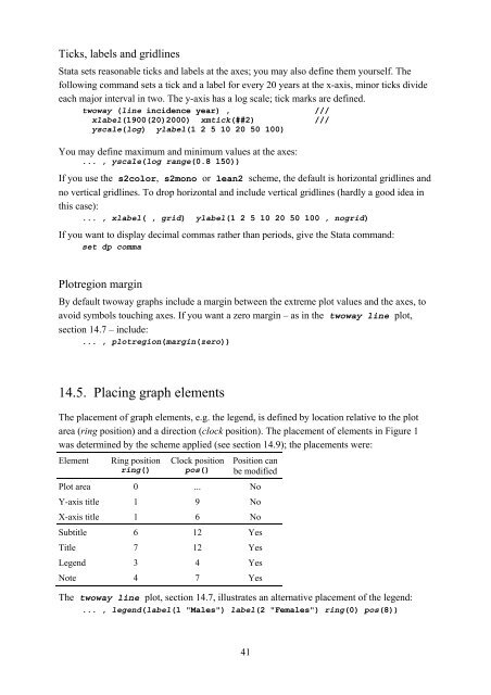
Ticks, labels and gridlines
Stata sets reasonable ticks and labels at the axes; you may also define them yourself. The
following command sets a tick and a label for every 20 years at the x-axis, minor ticks divide
each major interval in two. The y-axis has a log scale; tick marks are defined.
twoway (line incidence year) , ///
xlabel(1900(20)2000) xmtick(##2) ///
yscale(log) ylabel(1 2 5 10 20 50 100)
You may define maximum and minimum values at the axes:
... , yscale(log range(0.8 150))
If you use the s2color, s2mono or lean2 scheme, the default is horizontal gridlines and
no vertical gridlines. To drop horizontal and include vertical gridlines (hardly a good idea in
this case):
... , xlabel( , grid) ylabel(1 2 5 10 20 50 100 , nogrid)
If you want to display decimal commas rather than periods, give the Stata command:
set dp comma
Plotregion margin
By default twoway graphs include a margin between the extreme plot values and the axes, to
avoid symbols touching axes. If you want a zero margin – as in the twoway line plot,
section 14.7 – include:
... , plotregion(margin(zero))
14.5. Placing graph elements
The placement of graph elements, e.g. the legend, is defined by location relative to the plot
area (ring position) and a direction (clock position). The placement of elements in Figure 1
was determined by the scheme applied (see section 14.9); the placements were:
Element Ring position
ring()
Clock position
pos()
Position can
be modified
Plot area 0 ... No
Y-axis title 1 9 No
X-axis title 1 6 No
Subtitle 6 12 Yes
Title 7 12 Yes
Legend 3 4 Yes
Note 4 7 Yes
The twoway line plot, section 14.7, illustrates an alternative placement of the legend:
... , legend(label(1 "Males") label(2 "Females") ring(0) pos(8))
41