shot noise in mesoscopic conductors - Low Temperature Laboratory

More documents

Recommendations

Info

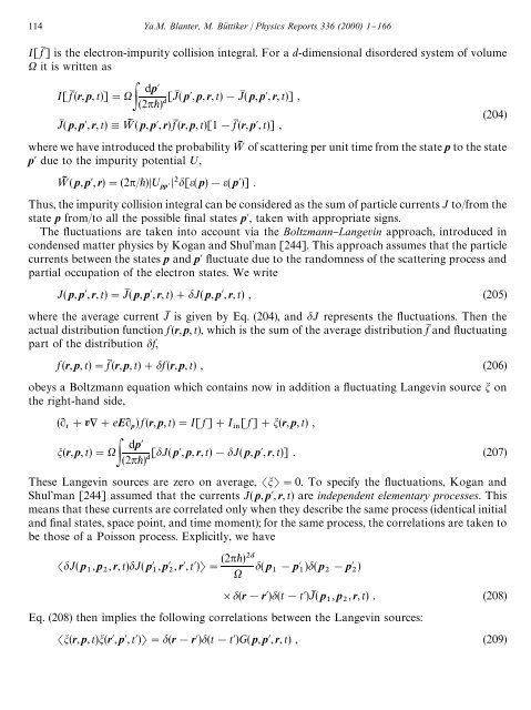
114 Ya.M. Blanter, M. Bu( ttiker / Physics Reports 336 (2000) 1}166 I[ fM ] is the electron-impurity collision integral. For a d-dimensional disordered system of volume it is written as dp I[ fM (r, p, t)]" [JM ( p, p, r, t)!JM ( p, p, r, t)] , (2) (204) JM ( p, p, r, t),=I ( p, p, r) fM (r, p, t)[1!fM (r, p, t)] , where we have introduced the probability =I of scattering per unit time from the state p to the state p due to the impurity potential ;, =I ( p, p, r)"(2/); pp [( p)!( p)] . Thus, the impurity collision integral can be considered as the sum of particle currents J to/from the state p from/to all the possible "nal states p, taken with appropriate signs. The #uctuations are taken into account via the Boltzmann}Langevin approach, introduced in condensed matter physics by Kogan and Shul'man [244]. This approach assumes that the particle currents between the states p and p #uctuate due to the randomness of the scattering process and partial occupation of the electron states. We write J( p, p, r, t)"JM ( p, p, r, t)#J( p, p, r, t) , (205) where the average current JM is given by Eq. (204), and J represents the #uctuations. Then the actual distribution function f (r, p, t), which is the sum of the average distribution fM and #uctuating part of the distribution f, f (r, p, t)"fM (r, p, t)#f (r, p, t) , (206) obeys a Boltzmann equation which contains now in addition a #uctuating Langevin source on the right-hand side, (R #*#eER p) f (r, p, t)"I[ f ]#I [ f ]#(r, p, t) , dp (r, p, t)" [J( p, p, r, t)!J( p, p, r, t)] . (207) (2) These Langevin sources are zero on average, "0. To specify the #uctuations, Kogan and Shul'man [244] assumed that the currents J( p, p, r, t) are independent elementary processes. This means that these currents are correlated only when they describe the same process (identical initial and "nal states, space point, and time moment); for the same process, the correlations are taken to be those of a Poisson process. Explicitly, we have J( p , p , r, t)J( p , p , r, t)" (2) ( p !p )( p !p ) (r!r)(t!t)JM ( p , p , r, t) . (208) Eq. (208) then implies the following correlations between the Langevin sources: (r, p, t)(r, p, t)"(r!r)(t!t)G( p, p, r, t) , (209)
where Ya.M. Blanter, M. Bu( ttiker / Physics Reports 336 (2000) 1}166 115 G( p, p, r, t)" ( p!p) dp[JM ( p, p, r, t)#JM ( p, p, r, t)] ! [JM ( p, p, r, t)#JM ( p, p, r, t)] . (210) Note that the sum rule dp G( p, p, r, t)" dp G( p, p, r, t)"0 (211) is ful"lled. This sum rule states that the #uctuations only redistribute the electrons over di!erent states, but do not change the total number of particles. These equations can be further simpli"ed in the important case (which is the main interest in this Section) when all the quantities are sharply peaked around the Fermi energy. Instead of the momentum p, we introduce then the energy E and the direction of the momentum n"p/p. The velocity and the density of states are assumed to be constant and equal to v and , respectively. We write =I ( p, p, r)"(E!E)=(n, n, r) , where = is the probability of scattering from the state n to the state n per unit time at the space point r. Furthermore, we will be interested only in the stationary regime, i.e. the averages fM and JM (not the #uctuating parts) are assumed to be time independent. Eliminating the electric "eld E by the substitution EPE!e(r), with being the potential, we write the Boltzmann}Langevin equation in the form (R #v n) f (r, n, E, t)"I[ f ]#I [ f ]#(r, n, E, t) , (212) where the Langevin sources are zero on average and are correlated as follows: (r, n, E, t)(r, n, E, t)" 1 (r!r)(t!t)(E!E)G(n, n, r, E) , (213) G(n, n, r, E), dn[(n!n)!(n!n)] [=(n, n, r) fM (1!fM )#=(n, n, r) fM (1!fM )] . (214) We used the notations fM ,fM (r, n, E) and fM ,fM (r, n, E). The expression for the current density, j(r, t)"ev dn dE nf (r, n, E, t) (215) (with the normalization dn"1), completes the system of equations used in the Boltzmann} Langevin method. We remark that in this formulation the local electric potential does not appear explicitly: for systems with charged carriers such as electric conductors the electric "eld is coupled to the (#uctuating) charge density via the Poisson equation. We will return to this point when we discuss situations in which a treatment of this coupling is essential.
Page 1 and 2:
Ya.M. Blanter, M. BuK ttiker / Phys
Page 3 and 4:
8. Concluding remarks, future prosp
Page 5 and 6:
text; they are usually extensions o
Page 7 and 8:
such reviews are not readily availa
Page 9 and 10:
Ya.M. Blanter, M. Bu( ttiker / Phys
Page 11 and 12:
The above considerations are, of co
Page 13 and 14:
Page 15 and 16:
Page 17 and 18:
and the initial state of our two-pa
Page 19 and 20:
Page 21 and 22:
Page 23 and 24:
2.3.3. Multi-terminal case We consi
Page 25 and 26:
Note that in the absence of time-de
Page 27 and 28:
Page 29 and 30:
equilibrium and shot noise. For low
Page 31 and 32:
Page 33 and 34:
Page 35 and 36:
Page 37 and 38:
Page 39 and 40:
and S" e A e< dE ¹(E )[1!¹
Page 41 and 42:
arrier, situated in the region !w/2
Page 43 and 44:
Page 45 and 46:
Page 47 and 48:
we include weak localization e!ects
Page 49 and 50:
Page 51 and 52:
Page 53 and 54:
Page 55 and 56:
Page 57 and 58:
Page 59 and 60:
Edge channels in the quantum Hall e
Page 61 and 62:
Fig. 19. (a) Geometry of a ring thr
Page 63 and 64: a manifestation of interference e!e
Page 65 and 66: Ya.M. Blanter, M. Bu( ttiker / Phys
Page 69 and 70: Physically, this corresponds to ele
Page 73 and 74: Our starting point is Eq. (51), whi
Page 77 and 78: introducing the transmission coe$ci
Page 79 and 80: investigated experimentally. A self
Page 85 and 86: and the non-equilibrium resistance
Page 87 and 88: the sample. These electrons are des
Page 93 and 94: with D ,¹ (2!¹ ). Performing t
Page 97 and 98: For completeness, we mention that i
Page 107 and 108: We note here, however, that there i
Page 111 and 112: The noise power (201) is strongly v
Page 113: Fig. 32. Experimental results of Ku
Page 117 and 118: where the quantity is expressed th
Page 119 and 120: 6.3. Interaction ewects Ya.M. Blant
Page 123 and 124: one "rst goes from the non-interact
Page 125 and 126: non-thermalized electrons, the high
Page 129 and 130: Fig. 34. Geometry of the chaotic ca
Page 133 and 134: which describes strictly ballistic
Page 141 and 142: approximately e/C. Between the peak
Page 149 and 150: Boltzmann}Langevin approach (see Se
Page 151 and 152: thermal to shot noise. It is, howev
Page 153 and 154: Note added in proof Ya.M. Blanter,
Page 155 and 156: and Lee et al. [340] obtain in this
Page 165 and 166:
show all

shot noise in mesoscopic conductors - Low Temperature Laboratory

Create successful ePaper yourself

Delete template?

Save as template?