Download - NASA

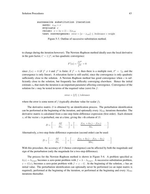
Solution Procedures 43
successive substitution iteration
save: xold = x
evaluate x
relax: x = λx +(1− λ)xold
test convergence: error = x − xold ≤λtolerance × weight
Figure 5-3. Outline of successive-substitution method.
to change during the iteration however). The Newton–Raphson method ideally uses the local derivative
in the gain factor, C =1/f ′ , so has quadratic convergence:
F ′ (α) = ff′′
=0
f ′2
since f(α) =0(if f ′ = 0and f ′′ is finite; if f ′ =0, then there is a multiple root, F ′ = 1/2, and the
convergence is only linear). A relaxation factor is still useful, since the convergence is only quadratic
sufficiently close to the solution. A Newton–Raphson method has good convergence when x is sufficiently
close to the solution, but frequently has difficulty converging elsewhere. Hence the initial
estimate x0 that starts the iteration is an important parameter affecting convergence. Convergence of the
solution for x may be tested in terms of the required value (zero) for f:
error = f ≤tolerance
where the error is some norm of f (typically absolute value for scalar f).
The derivative matrix D is obtained by an identification process. The perturbation identification
can be performed at the beginning of the iteration, and optionally every MPID iterations thereafter. The
derivative matrix is calculated from a one-step finite-difference expression (first order). Each element
xi of the vector x is perturbed, one at a time, giving the i-th column of D:
D =
···
∂f
∂xi
··· = ···
f(xi + δxi) − f(xi)
Alternatively, a two-step finite-difference expression (second order) can be used:
D =
···
∂f
∂xi
··· = ···
δxi
f(xi + δxi) − f(xi − δxi)
With this procedure, the accuracy of D (hence convergence) can be affected by both the magnitude and
sign of the perturbation (only the magnitude for a two-step difference).
The process for the Newton–Raphson method is shown in Figure 5-4. A problem specified as
h(x) =htarget becomes a zero-point problem with f = h − htarget. A successive-substitution problem,
x = G(x), becomes a zero-point problem with f = x − G. At the beginning of the solution, x has an
initial value. The perturbation identification can optionally never be performed (so an input matrix is
required), performed at the beginning of the iteration, or performed at the beginning and every MPID
iterations thereafter.
2δxi
···
···