Algorithm Design

210
Chapter 5 Divide and Conquer 5.1 A First Recurrence: The Mergesort Algorithm 211
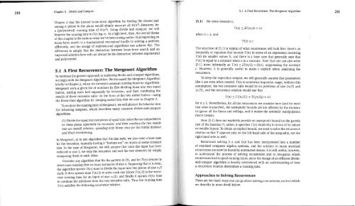
Chapter 2 that the natural brute-force algorithm for finding the closest pair
among n points in the plane would simply measure all ® (n 2) distances, for
a (polynomial) running time of O(n2). Using divide and conquer, we wi!!
improve the running time to O(n log n). At a high level, then, the overall theme
of this chapter is the same as what we’ve been seeing earlier: that improving on
brute-force search is a fundamental conceptual hurdle in solving a problem
efficiently, and the design of sophisticated algorithms can achieve this. The
difference is simply that the distinction between brute-force search and an
improved solution here will not always be the distinction between exponential
and polynomia!.
5.1 A First Recurrence: The Mergesort Algorithm
To motivate the general approach to analyzing divide-and-conquer algorithms,
we begin with the Mergesort Algorithm. We discussed the Mergesort Algorithm
briefly in Chapter 2, when we surveyed common running times for algorithms.
Mergesort sorts a given list of numbers by first diviiting them into two equal
halves, sorting each half separately by recursion, and then combining the
results of these recursive calls--in the form of the two sorted halves--using
the linear-time algorithm for merging sorted lists that we saw in Chapter 2.
To analyze the running time of Mergesort, we will abstract its behavior into
the following template, which describes many common divide-and-conquer
algorithms.
(Q Divide the input into two pieces of equal size; solve the two subproblems
on these pieces separately by recursion; and then combine the two results
into an overall solution, spending only linear time for the initial division
and final recombining.
In Mergesort, as in any algorithm that fits this style, we also need a base case
for the recursion, typically having it "bottom out" on inputs of some constant
size. In the case of Mergesort, we will assume that once the input has been
reduced to size 2, we stop the- recursion and sort the two elements by simply
comparing them to each other.
Consider any algorithm that fits the pattern in (J-), and let T(n) denote its
worst-case running time on input instances of size n. Supposing that n is even,
the algorithm spends O(n) time to divide the input into two pieces of size n/2
each; it then spends time T(n/2) to solve each one (since T(n/2) is the worstcase
nmning time for an input of size n/2); and finally it spends O(n) time
to combine the solutions from the two recursive calls. Thus the running time
T(n) satisfies the following recurrence relation.
(5.1) For some constant c,
when n > 2, and
T(n) < 2T(n/2) + cn
T(2) _< c.
The structure of (5.1) is typical of what recurrences will look like: there’s an
inequality or equation that bounds T(n) in terms of an expression involving
T(k) for sma!ler values k; and there is a base case that generally says that
T(n) is equal to a constant when n is a constant. Note that one can also write
(5.1) more informally as T(n)< 2T(n/2)+ O(n), suppressing the constant
c. However, it is generally useful to make c explicit when analyzing the
recurrence.
To keep the exposition simpler, we will generally assume that parameters
like n are even when needed. This is somewhat imprecise usage; without this
assumption, the two recursive calls would be on problems of size In/2] and
[n/2J, and the recurrence relation would say that
T(n) < T([n/2]) + T(Ln/2J) + cn
for n > 2. Nevertheless, for all the recurrences we consider here (and for most
that arise in practice), the asymptotic bounds are not affected by the decision
to ignore all the floors and ceilings, and it makes the symbolic manipulation
much cleaner.
Now (5.1) does not exphcitly provide an asymptotic bound on the growth
rate of the function T; rather, it specifies T(n) implicitly in terms of its values
on smaller inputs. To obtain an explicit bound, we need to solve the recurrence
relation so that T appears only on the left-hand side of the inequality, not the
fight-hand side as well.
Recurrence solving is a task that has been incorporated into a number
of standard computer algebra systems, and the solution to many standard
recurrences can now be found by automated means. It is still useful, however,
to understand the process of solving recurrences and to recognize which
recurrences lead to good running times, since the design of an efficient divideand-conquer
algorithm is heavily intertwined with an understanding of how
a recurrence relation determines a running time.
Approaches to Solving Recurrences
There are two basic ways one can go about solving a recurrence, each of which
we describe in more detail below.