Algorithm Design

54O
Chapter 7 Network Flow
define fout (S) = ~e out of S f(e) and fin(s) ---- ~e into $ f(e). In this terminology,
the conservation condition for nodes v ~ s, t becomes fin(v) = f°ut(v); and we
can write v(f) = f°Ut(s).
The Maximum-Flow Problem Given a flow network, a natural goa! is to
arrange the traffic so as to make as efficient use as possible of the available
capacity. Thus the basic algorithmic problem we will consider is the following:
Given a flow network, find a flow of maximum possible value.
As we think about designing algorithms for this problem, it’s useful to
consider how the structure of the flow network places upper bounds on the
maximum value of an s-t flow. Here is a basic "obstacle" to the existence of
large flows: Suppose we divide the nodes of the graph into two sets, A and
B, so that s ~ A and t ~ B. Then, intuitively, any flow that goes from s to t
must cross from A into B at some point, and thereby use up some of the edge
capacity from A to B. This suggests that each such "cut" of the graph puts a
bound on the maximum possible flow value. The maximum-flow algori_thm
that we develop here will be intertwined with a proof that the maximum-flow
value equals the minimum capacity of any such division, called the minimum
cut. As a bonus, our algorithm wil! also compute the minimum cut. We will
see that the problem of finding cuts of minimum capacity in a flow network
turns out to be as valuable, from the point of view of applications, as that of
finding a maximum flow.
~ Designing the Algorithm
Suppose we wanted to find a maximum flow in a network. How should we
go about doing this~. It takes some testing out to decide that an approach
such as dynamic programming doesn’t seem to work--at least, there is no
algorithm known for the Maximum-Flow Problem that could really be viewed
as naturally belonging to the dynamic programming paradigm. In the absence
of other ideas, we could go back and think about simple greedy approaches,
to see where they break down.
Suppose we start with zero flow: f(e) = 0 for al! e. Clearly this respects the
capacity and conservation conditions; the problem is tha~ its value is 0. We
now try to increase the value of f by "pushing" flow along a path from s to t,
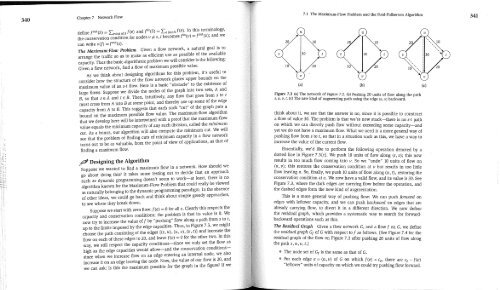
up to the limits imposed by the edge capacities. Thus, in Figure 7.3, we might
choose the path consisting of the edges {(s, u), (u, ~), (~, t)} and increase the
flow on each of these edges to 20, and leave f(e) = 0 for the other two. In this
way, we still respect the capacity conditions--since we only set the flow as
high as the edge capacities would allow--and the conservation conditions-since
when we increase flow on an edge entering an internal node, we also
increase it on an edge leaving the node. Now, the value of our flow is 20, .and
we can ask: Is this the maximum possible for the graph in the figure? If we
7.1 The Maximum-Flow Problem and the Ford-Fulkerson Algorithm
10
2O
(a) (b)
Figure 7.3 (a) The network of Hgure 7.2. Co) Pushing 20 units of flow along the path
s, u, v, t. (c) The new kind of augmenting path using the edge (u, v) backward.
think about it, we see that the answer is no, since it is possible to construct
a flow of value 30. The problem is that we’re now stuck--there is no s-t patii
on which we can directly push flow without exceeding some capacity--and
yet we do not have a maximum flow. What we need is a more general way of
pushing flow from s to t, so that in a situation such as this, we have a way to
increase the value of the current flow.
Essentially, we’d like to perform the following operation denoted by a
dotted line in Figure 7.3(c). We push 10 units of flow along (s, v); this now
results in too much flow coming into v. So we "undo" 10 units of flow on
(u, v); this restores the conservation condition at v but results in too little
flow leaving u. So, finally, we push 10 units of flow along (u, t), restoring the
conservation condition at u. We now have a valid flow, and its value is 30. See
Figure 7.3, where the dark edges are carrying flow before the operation, and
the dashed edges form the new kind of augmentation.
This is a more general way of pushing flow: We can push forward on
edges with leftover capacity, and we can push backward on edges that are
already caning flow, to divert it in a different direction. We now define
the residual graph, which provides a systematic way to search for forwardbackward
operations such as this.
The Residual Graph Given a flow network G, and a flow f on G, we define
the residual graph Gf of G with respect to f as follows. (~ee Figure 7.4 for the
residual graph of the flow on Figure 7.3 after pushing 20 units of flow along
the path s, u, v, t.)
The node set of Gf is the same as that of G.
For each edge e = (u, v) of G on which f(e) < c e, there are ce- f(e)
"leftover" units of capacity on which we could try pushing flow forward.
10
341