Algorithm Design

148
Chapter 4 Greedy Algorithms
~Tcan be swapped for e.)
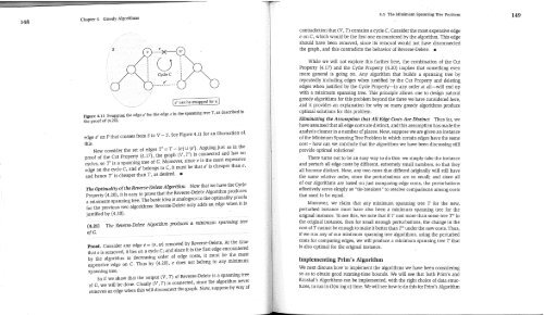
Figure 4.11 Swapping the edge e’ for the edge e in the spanning tree T, as described in
the proof of (4.20).
edge e’ on P that crosses from S to V - S. See Figure 4.11 for an illustration of,
this.
Now consider the set of edges T ~ = T - {e} LJ [e’}. Arguing just as in the
proof of the Cut Property (4.17), the graph (V, T ~) is connected and has no
cycles, so T’ is a spanning tree of G. Moreover, since e is the most expensive
edge on the cycle C, and e’ belongs to C, it must be that e’ is cheaper than e,
and hence T’ is cheaper than T, as desired. []
The Optimality of the Reverse-Delete Algorithm Now that we have the Cycle
Property (4.20), it is easy to prove that the Reverse-Delete Algorithm produces
a minimum spanning tree. The basic idea is analogous to the optimality proofs
for the previous two algorithms: Reverse-Delete only adds an edge when it is
justified by (4.20).
(4.21) The Reverse-Delete Algorithm produces a minimum spanning tree
of G.
Proof. Consider any edge e = (v, w) removed by Reverse-Delete. At the time
that e is removed, it lies on a cycle C; and since it is the first edge encountered
by the algorithm in decreasing order of edge costs, it must be the most
expensive edge on C. Thus by (4.20), e does not belong to any minimum
spanning tree.
So if we show that the output (V, T) of Reverse-Delete is a spanning tree
of G, we will be done. Clearly (V, T) is connected, since the algorithm never
removes an edge when this will disconnect the graph. Now, suppose by way of
4.5 The Minimum Spanning Tree Problem
contradiction that (V, T) contains a cycle C. Consider the most expensive edge
e on C, which would be the first one encountered by the algorithm. This e.dge
should have been removed, since its removal would not have disconnected
the graph, and this contradicts the behavior of Reverse-Delete. []
While we will not explore this further here, the combination of the Cut
Property (4.17) and the Cycle Property (4.20) implies that something even
more general is going on. Any algorithm that builds a spanning tree by
repeatedly including edges when justified by the Cut Property and deleting
edges when justified by the Cycle Property--in any order at all--will end up
with a minimum spanning tree. This principle allows one to design natural
greedy algorithms for this problem beyond the three we have considered here,
and it provides an explanation for why so many greedy algorithms produce
optimal solutions for this problem.
Eliminating the Assumption that All Edge Costs Are Distinct Thus far, we
have assumed that all edge costs are distinct, and this assumption has made the
analysis cleaner in a number of places. Now, suppose we are given an instance
of the Minimum Spanning Tree Problem in which certain edges have the same
cost - how can we conclude that the algorithms we have been discussing still
provide optimal solutions?
There turns out to be an easy way to do this: we simply take the instance
and perturb all edge costs by different, extremely small numbers, so that they
all become distinct. Now, any two costs that differed originally will sti!l have
the same relative order, since the perturbations are so small; and since all
of our algorithms are based on just comparing edge costs, the perturbations
effectively serve simply as "tie-breakers" to resolve comparisons among costs
that used to be equal.
Moreover, we claim that any minimum spanning tree T for the new,
perturbed instance must have also been a minimum spanning tree for the
original instance. To see this, we note that if T cost more than some tree T* in
the original instance, then for small enough perturbations, the change in the
cost of T cannot be enough to make it better than T* under the new costs. Thus,
if we run any of our minimum spanning tree algorithms, using the perturbed
costs for comparing edges, we will produce a minimum spanning tree T that
is also optimal for the original instance.
Implementing Prim’s Algorithm
We next discuss how to implement the algorithms we have been considering
so as to obtain good running-time bounds. We will see that both Prim’s and
Kruskal’s Algorithms can be implemented, with the right choice of data structures,
to run in O(m log n) time. We will see how to do this for Prim’s Algorithm
149