Algorithm Design

238
Chapter 5 Divide and Conquer
Could one design an algorithm that bypasses the quadratic-size definition of
convolution and computes it in some smarter way?
In fact, quite surprisingly, this is possible. We now describe a method
that computes the convolution of two vectors using only O(n log n) arithmetic
operations. The crux of this method is a powerful technique known as the Fast
Fourier Transform (FFT). The FFT has a wide range of further applications in
analyzing sequences of numerical values; computing convolutions quickly,
which we focus on here, is iust one of these applications.
~ Designing and Analyzing the Algorithm
To break through the quadratic time barrier for convolutions, we are going
to exploit the connection between the convolution and the multiplication of
two polynomials, as illustrated in the first example discussed previously. But
rather than use convolution as a primitive in polynomial multiplication, we
are going to exploit this connection in the opposite direction.
Suppose we are given the vectors a = (ao, al ..... an_~) and b= (bo,,
bn_l). We will view them as the polynomials A(x) = a o + alx + a2x 2 +
¯ . ¯ an_~x n-~ and B(x) = bo + b~x + b2 x2 ÷" "" bn-1 xn-1, and we’ll seek to compute
their product C(x) = A(x)B(x) in O(n log rt) time. If c = (Co, c~ .... , c2n_2)
is the vector of coefficients of C, then we recall from our earlier discussion
that c is exactly the convolution a ¯ b, and so we can then read off the desired
answer directly from the coefficients of C(x).
Now, rather than multiplying A and B symbolically, we can treat them as
functions of the variable x and multiply them as follows.
(i)
(ii)
(iii)
First we choose 2n values xl, x 2 ..... x2n and evaluate A(xj) and B(xj) for
each of j = !, 2 ..... 2n.
We can now compute C(xi) for each ] very easily: C(xj) is simply the
product of the two numbers A(xj) and B(xj).
Finally, we have to recover C from its values on x~, x2 ..... x2n. Here we
take advantage of a fundamental fact about polynomials: any polynomial
of degree d can be reconstructed from its values on any set of d + 1 or
more points. This is known as polynomial interpolation, and we’ll discuss
the mechanics of performing interpolation in more detail later. For the
moment, we simply observe that since A and B each have degree at
most n - !, their product C has degree at most 2n - 2, and so it can be
C(x2n) that we computed
reconstructed from the values C(xl), C(x2) .....
in step (ii).
This approach to multiplying polynomials has some promising aspects
and some problematic ones. First, the good news: step (ii) requires only
: 5.6 Convolutions and the Fast Fourier Transform 239
O(n) arithmetic operations, since it simply involves the multiplication of O(n)
numbers. But the situation doesn’t look as hopeful with steps (i) and (fii). In
particular, evaluating the polynomials A and B on a single value takes S2 (n)
operations, and our plan calls for performing 2n such evaluations. This seems
to bring us back to quadratic time right away.
The key idea that will make this all work is to find a set of 2n values
x~, x2 ..... x2n that are intimately related in some way, such that the work in
evaluating A and B on all of them can be shared across different evaluations. A
set for which this wil! turn out to work very well is the complex roots o[ unity.
The Complex Roots of Unity At this point, we’re going to need-to recal! a
few facts about complex numbers and their role as solutions to polynomial
equations.
Recall that complex numbers can be viewed as lying in the "complex
plane," with axes representing their real and imaginary parts. We can write
a complex number using polar coordinates with respect to this plane as re °i,
where e’r~= -1 (and e2’-n = 1). Now, for a positive integer k, the polynomial
equation x k = 1 has k distinct complex roots, and it is easy to identify them.
Each of the complex numbers wj,k = e 2’-qi/k (for] = 0, 1, 2 ..... k - 1) satisfies
the equation, since
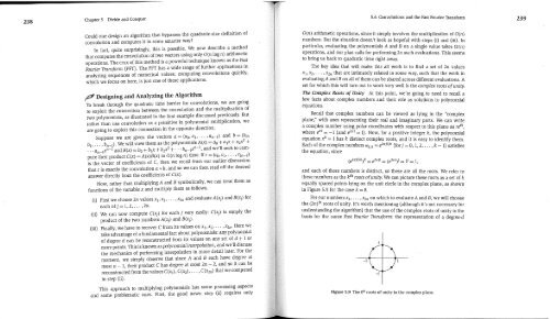
and each of these numbers is distinct, so these are all the roots. We refer to
these numbers as the k th roots of unity. We can picture these roots as a set of k
equally spaced points lying on the unit circle in the complex plane, as shown
in Figure 5.9 for the case k = 8.
For our numbers x~ ..... x2n on which to evaluate A and B, we will choose
the (2n) th roots of unity. It’s worth mentioning (although it’s not necessary for
understanding the algorithm) that the use of the complex roots of unity is the
basis for the name Fast Fourier Transform: the representation of a degree-d
Figure 5.9 The 8 th roots of unity in the complex plane.