

Algorithm Design
Algorithm Design
Algorithm Design

Create successful ePaper yourself
Turn your PDF publications into a flip-book with our unique Google optimized e-Paper software.
294<br />
t<br />
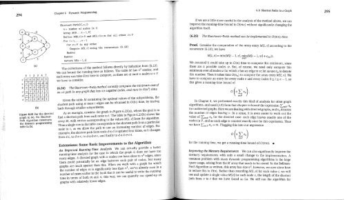
Ca)<br />
0 1 2 3 4 5<br />
3<br />
0 -2 -2 -2<br />
3 3 3<br />
3 3 2<br />
0 0 I o 0<br />
Co)<br />
Figure 6.23 For the directed<br />
graph in (a), the Shortest-<br />
Path <strong>Algorithm</strong> constructs<br />
the dynamic programming<br />
table in (b).<br />
Chapter 6 Dynamic Programming<br />
Shortest-Path (G, s, t)<br />
~= number of nodes in G<br />
Array M[O...n- I, V]<br />
Define M[O,t]=O and M[O,u]=oo for all other u~V<br />
For i_--l,...,n-I<br />
For u~V in any order<br />
Compute A4[i, v] using the recurrence (6.23)<br />
Endfor<br />
Enddor<br />
Return M[~t -- I, S]<br />
The correctness of the method follows directly by induction from (6.23).<br />
We can bound the running time as follows. The table M has n 2 entries; and<br />
each entry can take O(n) time to compute, as there are at most n nodes w ~ V<br />
we have to consider.<br />
(6.24) The Shortest-Path method correctly computes the minimum cost.of<br />
an s-t path in any graph that has no negative cycles, and runs fn O(n 3) time.<br />
Given the table M containing the optimal values of the subproblems, the<br />
shortest path using at most i edges can be obtained in O(in) time, by tracing<br />
back through smaller subproblems.<br />
As an example, consider the graph in Figure 6.23 (a), where the goal is to<br />
find a shortest path from each node to t. The table in Figure 6.23 (b) shows the<br />
array M, with entries corresponding to the values M[i, v] from the algorithm.<br />
Thus a single row in the table corresponds to the shortest path from a particular<br />
node to t, as we allow the path to use an increasing number of edges. For<br />
example, the shortest path from node d to t is updated four times, as it changes<br />
from d-t, to d-a-t, to d-a-b-e-t, and finally to d-a-b-e-c-t.<br />
Extensions: Some Basic Improvements to the <strong>Algorithm</strong><br />
An Improved Running-Time Analysis We can actually provide a better<br />
running-time analysis for the case in which the graph G does not have too<br />
many edges. A directed graph with n nodes can have close to n 2 edges, since<br />
there could potentially be an edge between each pair of nodes, but many<br />
graphs are much sparser than this. When we work with a graph for which<br />
the number of edges m is significantly less than n z, we’ve already seen in a<br />
number of cases earlier in the book that it can be useful to write the runningtime<br />
in terms of both m and n; this way, we can quantify our speed-up on<br />
graphs with relatively fewer edges.<br />
6.8 Shortest Paths in a Graph<br />
If we are a little more careful in the analysis of the method above, we can<br />
improve the running-time bound to O(mn) without significantly changing the<br />
algorithm itself.<br />
The Shoz~ZesZ2Path method can be implemented in O(mn) time:<br />
Proof. Consider the computation of the array entry M[i, v] according to the<br />
recurrence (6.23);. we have<br />
M[i, v] = min(M[i - 1, v], min(M[i -- 1, w] + cu~)).<br />
tu~V<br />
We assumed it could take up to O(n) time to compute this minimum, since<br />
there are n possible nodes w. But, of course, we need only compute this<br />
minimum over all nodes w for which v has an edge to w; let us use n u to denote<br />
this number. Then it takes time O(nu) to compute the array entry M[i, v]. We<br />
have to compute an entry for every node v and every index 0 < i < n - 1, so<br />
this gives a running-time bound of<br />
In Chapter 3, we performed exactly this kind of analysis for other graph<br />
algorithms, and used (3.9) from that chapter to bound the expression ~usv nu<br />
for undirected graphs. Here we are dealing with directed graphs, and nv denotes<br />
the number of edges leaving v. In a sense, it is even easier to work out the<br />
value of ~v,v nu for the directed case: each edge leaves exactly one of the<br />
nodes in V, and so each edge is counted exactly once by this expression. Thus<br />
we have ~u~v n~ = m. Plugging this into our expression<br />
for the running time, we get a running-time bound of O(mn).<br />
Improving the Memory Requirements We can also significantly improve the<br />
memory requirements with only a small change to the implementation. A<br />
common problem with many dynamic programming algorithms is the large<br />
space usage, arising from the M array that needs to be stored. In the Bellman-<br />
Ford <strong>Algorithm</strong> as written, this array has size n2; however, we now show how<br />
to reduce this to O(n). Rather than recording M[i, v] for each value i, we will<br />
use and update a single value M[v] for each node v, the length of the shortest<br />
path from v to t that we have found so far. We still run the algorithm for<br />
295


