Algorithm Design

140
Chapter 4 Greedy Algorithms
Set S
lth
The alternate s-v path P through~
x and y is already too long by |
e time it has left the set S, )
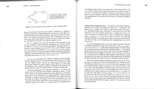
Figure 4.8 The shortest path Pv and an alternate s-v path P through the node
long as Pv by the time it has left the set S. Indeed, in iteration k + 1, Dijkstra’s
Algorithm must have considered adding node y to the set S via the edge (x, y)
and rejected this option in favor of adding u. This means that there is no path
from s to y through x that is shorter than Pv- But the subpath of P up to y is
such a path, and so this subpath is at least as long as P,. Since edge length~
are nonnegative, the full path P is at least as long as P, as well.
This is a complete proof; one can also spell out the argument in the
previous paragraph using the following inequalities. Let P’ be the Subpath
of P from s to x. Since x ~ S, we know by the induction hypothesis that Px is a
shortest s-x path (of length d(x)), and so g(P’) > g(Px) = d(x). Thus the subpath
of P out to node y has length ~(P’) + g(x, y) > d(x) + g.(x, y) > d’(y), and the
full path P is at least as long as this subpath. Finally, since Dijkstra’s Algorithm
selected u in this iteration, we know that d’(y) >_ d’(u) = g(Pv). Combining these
inequalities shows that g(P) >_ ~(P’) + ~.(x, y) >_ g(P~). ’~
Here are two observations about Dijkstra’s Algorithm and its analysis.
First, the algorithm does not always find shortest paths if some of the edges
can have negative lengths. (Do you see where the proof breaks?) Many
shortest-path applications involve negative edge lengths, and a more complex
algorithm--due to Bellman and Ford--is required for this case. We will
see this algorithm when we consider the topic of dynamic programming.
The second observation is that Dijkstra’s Algorithm is, in a sense, even
simpler than we’ve described here. Dijkstra’s Algorithm is really a "continuous"
version of the standard breadth-first search algorithm for traversing a
graph, and it can be motivated by the following physical intuition. Suppose
the edges of G formed a system of pipes filled with water, joined together at
the nodes; each edge e has length ge and a fixed cross-sectional area. Now
suppose an extra droplet of water falls at node s and starts a wave from s. As
the wave expands out of node s at a constant speed, the expanding sphere
4.4 Shortest Paths in a Graph
of wavefront reaches nodes in increasing order of their distance from s. It is
easy to believe (and also true) that the path taken by the wavefront to get to
any node u is a shortest path. Indeed, it is easy to see that this is exactly the
path to v found by Dijkstra’s Algorithm, and that the nodes are discovered by
the expanding water in the same order that they are discovered by Dijkstra’s
Algorithm.
Implementation and Running Time To conclude our discussion of Dijkstra’s
Algorithm, we consider its running time. There are n - 1 iterations of the
krt~±].e loop for a graph with n nodes, as each iteration adds a new node v
to S. Selecting the correct node u efficiently is a more subtle issue. One’s first
impression is that each iteration would have to consider each node v ~ S,
and go through all the edges between S and u to determine the minimum
mine=(u,u):u~ s d(u)+g-e, so that we can select the node v for which this
minimum is smallest. For a graph with m edges, computing all these minima
can take O(m) time, so this would lead to an implementation that runs in
O(mn) time.
We can do considerably better if we use the right data structures. First, we
will explicitly maintain the values of the minima d’(u) = mJne=(u,u):u~ s d(u) +
~e for each node v V - S, rather than recomputing them in each iteration.
We can further improve the efficiency by keeping the nodes V - S in a priority
queue with d’(u) as their keys. Priority queues were discussed in Chapter 2;
they are data structures designed to maintain a set of n elements, each with a
key. A priority queue can efficiently insert elements, delete elements, change
an element’s key, and extract the element with the minimum key. We will need
the third and fourth of the above operations: ChangeKey and Ex~cractN±n.
How do we implement Dijkstra’s Algorithm using a priority queue? We put
the nodes V in a priority queue with d’(u) as the key for u ~ V. To select the node
v that should be added to the set S, we need the Extrac~cN±n operation. To see
how to update the keys, consider an iteration in which node u is added to S, and
let tv ~ S be a node that remains in the priority queue. What do we have to do
to update the value of d’(w)? If (v, w) is not an edge, then we don’t have to do
anything: the set of edges considered in the minimum mihe=(u,w):a~ s d(u) + ~e
is exactly the same before and after adding v to S. If e’ = (v, w) ~ E, on
the other hand, then the new value for the key is min(d’(w), d(u) + ~-e’). If
d’(ro) > d(u) + ~e’ then we need to use the ChangeKey operation to decrease
the key of node w appropriately. This ChangeKey operation can occur at most
once per edge, when the tail of the edge e’ is added to S. In summary, we have
the following result.
141