Algorithm Design

482
Chapter 8 NP and Computational IntractabiliW
But this doesn’t help us establish the NP-completeness of B-Dimensional
Matching, since these reductions simply show that B-Dimensional Matching
can be reduced to some very hard problems. What we need to show is the other
direction: that a known NP-complete problem can be reduced to 3-Dimensional
Matching.
(8.20) 3,Dimensional Matching is NP-complete. ~
Proof. Not surprisingly, it is easy to prove that B-Dimensional Matching is in
:N~P. Given a collection of triples T C X x Y x Z, a certificate that there is a
solution could be a collection of triples T’ ~ T. In polynomial time, one could
verify that each element in X U Y u Z belongs to exactly one of the triples in T’.
For the reduction, we again return all the way to B-SAT. This is perhaps a
little more curious than in the case of Hamiltonian Cycle, since B-Dimensional
Matching is so closely related to both Set Packing and Set Cover; but in,fact the
partitioning requirement is very hard to encode using either of these problems.
Thus, consider an arbitrary instance of B-SAT, with n variables xl ..... Xn
and k clauses C1 ..... C k. We will show how to solve it, given the ~ability to
detect perfect three-dimensional matchings.
The overall strategy in this reduction will be similar (at a very high level)
to the approach we followed in the reduction from 3-SAT to Hamiltonian Cycle.
We will first design gadgets that encode the independent choices involved in
the truth assignment to each variable; we will then add gadgets that encode
the constraints imposed by the clauses. In performing this construction, we
will initially describe all the elements in the 3-Dimensional Matching instance
simply as "elements;’ without trying to specify for each one whether it comes
from X, Y, or Z. At the end, we wil! observe that they naturally decompose
into these three sets.
Here is the basic gadget associated with variable xi. We define elements
Ai ={ail, ai2 ..... ai,2k} that constitute the core of the gadget; we define
2k,
elements Bi = {bn
bi,xk
..... } at the tips of the gadget. For eachj = 1, 2 .....
we define a triple tij = (aij, aij+l, bij), where we interpret addition modulo 2k.
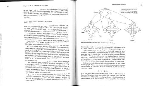
Three of these gadgets are pictured in Figure 8.9. In gadget i, we wil! call a
triple tij even if j is even, and odd if j is odd. In an analogous way, we will
refer to a tip bi~ as being either even or odd.
These will be the only triples that contain the elements in Ai, so we
can already say something about how they must be covered in any perfect
matching: we must either use al! the even triples in gadget i, or all the odd
triples in gadget i. This will be our basic way of encoding the idea that xi can
Clause 1
rips
Variable 1 Variable 2
Figure 8.9 The reduction from 3-SAT to 3-Dimensional Matching.
8.6 Partitioning Problems
I~
be set to either 0 or 1; if we select all the even triples, this will represent setting
x i = 0, and if we select all the odd triples, this wil! represent setting xi = 1.
Here is another way to view the odd/even decision, in terms of the tips of
the gadget. If we decide to use the even triples, we cover the even tips of the
gadget and leave the odd tips flee. If we decide to use the odd triples, we cover
the odd tips of the gadget and leave the even tips flee. Thus our decision of
how to set x i can be viewed as follows: Leaving the odd tips flee corresponds
to 0, while leaving the even tips flee corresponds to 1. This will actually be the
more useful way to think about things in the remainder of the construction.
So far we can make this even/odd choice independently for each of the n
variable gadgets. We now add elements to model the clauses and to constrain
the assignments we can choose. As in the proof of (8.17), let:s consider the
example of a clause
C1..~- X1V’~2 V X 3.
In the language of three-dimensional matchings, it tells us, "The matching on
the cores of the gadgets should leave the even tips of the first gadget flee; or it
should leave the odd tips of the second gadget flee; or it should leave the even
tips of the third gadget free." So we add a clause gadget that does precisely
he clause elements can only be ~
arched if some variable gadget |
eaves the corresponding tip flee..)
Variable 3
483