- Page 2 and 3:
Cornell University Boston San Franc
- Page 4 and 5:
Contents About the Authors Preface
- Page 6 and 7:
X Contents 9 10 Extending the Limit
- Page 8 and 9:
xiv Preface problems out in the wor
- Page 10 and 11:
Preface Chapters 2 and 3 also prese
- Page 12 and 13:
xxii Preface Preface xxiii Sue Whit
- Page 14 and 15:
2 Chapter 1 Introduction: Some Repr
- Page 16 and 17:
6 Chapter 1 Introduction: Some Repr
- Page 18 and 19:
10 Chapter 1 Introduction: Some Rep
- Page 20 and 21:
14 Chapter ! Introduction: Some Rep
- Page 22 and 23:
18 Chapter 1 Introduction: Some Rep
- Page 24 and 25:
22 Chapter 1 Introduction: Some Rep
- Page 26 and 27:
26 Chapter 1 Introduction: Some Rep
- Page 28 and 29:
30 Chapter 2 Basics of Algorithm An
- Page 30 and 31:
34 n= I0 n=30 n=50 = 100 = 1,000 10
- Page 32 and 33:
58 Chapter 2 Basics of Algorithm An
- Page 34 and 35:
42 Chapter 2 Basics of Algorithm An
- Page 36 and 37:
46 Chapter 2 Basics of Algorithm An
- Page 38 and 39:
50 Chapter 2 Basics of Algorithm An
- Page 40 and 41:
54 Chapter 2 Basics of Algorithm An
- Page 42 and 43:
58 Chapter 2 Basics of Algorithm An
- Page 44 and 45:
62 Chapter 2 Basics of Algorithm An
- Page 46 and 47:
66 Chapter 2 Basics of Algorithm An
- Page 48 and 49:
70 Chapter 2 Basics of Algorithm An
- Page 50 and 51:
74 Chapter 3 Graphs 3.1 Basic Defin
- Page 52 and 53:
78 Chapter 3 Graphs Rooted trees ar
- Page 54 and 55:
82 Chapter 3 Graphs Current compone
- Page 56 and 57:
86 Chapter 3 Graphs Proof. Suppose
- Page 58 and 59:
90 Chapter 3 Graphs Two of the simp
- Page 60 and 61:
94 Chapter 3 Graphs most ~u nv = 2m
- Page 62 and 63:
98 Chapter 3 Graphs It is important
- Page 64 and 65:
102 Chapter 3 Graphs ordering, that
- Page 66 and 67:
106 Chapter 3 Graphs We can already
- Page 68 and 69:
110 Chapter 3 Graphs Exercises 111
- Page 70 and 71:
Greedy A~gorithms In Wall Street, t
- Page 72 and 73:
118 Chapter 4 Greedy Mgofithms o In
- Page 74 and 75:
122 Chapter 4 Greedy Algorithms Our
- Page 76 and 77:
126 Chapter 4 Greedy Algorithms Len
- Page 78 and 79:
Before swapping: After swapping: d
- Page 80 and 81:
134 Chapter 4 Greedy Algorithms wit
- Page 82 and 83:
138 Chapter 4 Greedy Algorithms 4.4
- Page 84 and 85:
142 Chapter 4 Greedy Algorithms 4.5
- Page 86 and 87:
146 Chapter 4 Greedy Algorithms (e
- Page 88 and 89:
150 Chapter 4 Greedy Algorithms her
- Page 90 and 91:
154 Chapter 4 Greedy Algorithms we
- Page 92 and 93:
158 Chapter 4 Greedy Algorithms spa
- Page 94 and 95:
162 Chapter 4 Greedy Algorithms ~ T
- Page 96 and 97:
166 Chapter 4 Greedy Algorithms g2(
- Page 98 and 99:
170 Chapter 4 Greedy Algorithms Sha
- Page 100 and 101:
174 Chapter 4 Greedy Algorithms ...
- Page 102 and 103:
178 Chapter 4 Greedy Algorithms Fig
- Page 104 and 105:
182 Chapter 4 Greedy Algorithms The
- Page 106:
186 Chapter 4 Greedy Algorithms Sol
- Page 109 and 110:
192 Chapter 4 Greedy Algorithms 8.
- Page 111 and 112:
196 Chapter 4 Greedy Algorithms 15.
- Page 113 and 114:
200 Chapter 4 Greedy Algorithms 21.
- Page 115 and 116:
204 Chapter 4 Greedy Algorithms Not
- Page 117 and 118:
Chapter Divide artd Cortquer Divide
- Page 119 and 120:
212 Chapter 5 Divide and Conquer Th
- Page 121 and 122:
216 cn time plus recursive calls Ch
- Page 123 and 124:
220 Chapter 5 Divide and Conquer mo
- Page 125 and 126:
224 Chapter 5 Divide and Conquer El
- Page 127 and 128:
228 Chapter 5 Divide and Conquer 5.
- Page 129 and 130:
232 Chapter 5 Divide and Conquer (a
- Page 131 and 132:
we’ll just give a simple example
- Page 133 and 134:
240 Chapter 5 Divide and Conquer po
- Page 135 and 136:
244 Chapter 5 Divide and Conquer Th
- Page 137 and 138:
248 Chapter 5 Divide and Conquer It
- Page 139 and 140:
252 Chapter 6 Dynamic Programming b
- Page 141 and 142:
256 Chapter 6 Dynamic Programming 6
- Page 143 and 144:
260 Index 1 2 3 4 5 6 L~ I = 2 Chap
- Page 145 and 146:
264 Chapter 6 Dynamic Programming w
- Page 147 and 148:
268 Chapter 6 Dynamic Programming t
- Page 149 and 150:
272 Chapter 6 Dynamic Programming s
- Page 151 and 152:
276 Chapter 6 Dynamic Programming 1
- Page 153 and 154:
280 Chapter 6 Dynamic Programming t
- Page 155 and 156:
284 Figure 6.18 The OPT values for
- Page 157 and 158:
288 Chapter 6 Dynamic Programming U
- Page 159 and 160:
292 (a) Figure 6.21 (a) With negati
- Page 161 and 162:
296 Chapter 6 Dynamic Programming i
- Page 163 and 164:
300 Chapter 6 Dynamic Programming p
- Page 165 and 166:
304 Chapter 6 Dynamic Programming e
- Page 167 and 168:
308 Chapter 6 Dynamic Programming o
- Page 169 and 170:
312 Chapter 6 Dynamic Programming E
- Page 171 and 172:
316 Chapter 6 Dynamic Programming T
- Page 173 and 174:
320 Chapter 6 Dynamic Programming (
- Page 175 and 176:
324 Chapter 6 Dynamic Programming 1
- Page 177 and 178:
328 Chapter 6 Dynamic Programming T
- Page 179 and 180:
332 Chapter 6 Dynamic Programming 2
- Page 181 and 182:
336 Chapter 6 Dynamic Programming h
- Page 183 and 184:
54O Chapter 7 Network Flow define f
- Page 185 and 186:
344 Chapter 7 Network Flow This aug
- Page 187 and 188:
348 Chapter 7 Network Flow Proof. ~
- Page 189 and 190:
352 Chapter 7 Network Flow In the n
- Page 191 and 192:
356 Chapter 7 Network Flow (7.19) T
- Page 193 and 194:
360 Chapter 7 Network Flow preflow
- Page 195 and 196:
364 Chapter 7 Network Flow Heights
- Page 197 and 198:
368 Chapter 7 Network Flow ~ The Pr
- Page 199 and 200:
372 Chapter 7 Network Flow that are
- Page 201 and 202:
376 Chapter 7 Network Flow I~low ar
- Page 203 and 204:
380 Chapter 7 Network Flow Figure 7
- Page 205 and 206:
384 Chapter 7 Network Flow Lower bo
- Page 207 and 208:
388 BOS 6 DCA 7 DCA 8 Chapter 7 Net
- Page 209 and 210:
392 Chapter 7 Network Flow natural
- Page 211 and 212:
396 Chapter 7 Network Flow 7.11 Pro
- Page 213 and 214:
400 Chapter 7 Network Flow 7.12 Bas
- Page 215 and 216:
404 Chapter 7 Network Flow to cross
- Page 217 and 218:
4O8 Chapter 7 Network Flow Why are
- Page 219 and 220:
412 Chapter 7 Network Flow ProoL Th
- Page 221 and 222:
416 Chapter 7 Network Flow Figure 7
- Page 223 and 224:
420 Chapter 7 Network Flow 11. Now
- Page 225 and 226:
424 Figure 7.29 An instance of Cove
- Page 227 and 228:
428 Chapter 7 Network Flow 22. This
- Page 229 and 230:
432 Chapter 7 Network Flow generall
- Page 231 and 232:
436 Chapter 7 Network Flow (a) (b)
- Page 233 and 234:
440 Chapter 7 Network Flow going to
- Page 235 and 236:
Chapter 7 Network Flow 44. 45. Give
- Page 237 and 238:
448 Chapter 7 Network Flow 51. The
- Page 239 and 240:
452 Chapter 8 NP and Computational
- Page 241 and 242:
456 Chapter 8 NP and Computational
- Page 243 and 244:
460 Chapter 8 NP and Computational
- Page 245 and 246:
464 Chapter 8 NP and Computational
- Page 247 and 248:
468 Chapter 8 NP and Computational
- Page 249 and 250:
472 Chapter 8 NP and Computation!!
- Page 251 and 252:
476 Chapter 8 NP and Computational
- Page 253 and 254:
480 Chapter 8 NP and Computational
- Page 255 and 256:
484 Chapter 8 NP and Computational
- Page 257 and 258:
488 Chapter 8 NP and Computational
- Page 259 and 260:
492 Chapter 8 NP and Computational
- Page 261 and 262:
496 Chapter 8 NP and Computational
- Page 263 and 264:
5OO Chapter 8 NP and Computational
- Page 265 and 266:
504 Chapter 8 NP and Computational
- Page 267 and 268:
508 Chapter 8 NP and Computational
- Page 269 and 270:
512 Chapter 8 NP and Computational
- Page 271 and 272:
516 Chapter 8 NP and Computational
- Page 273 and 274:
520 Chapter 8 NP and Computational
- Page 275 and 276:
524 Chapter 8 NP and Computational
- Page 277 and 278:
528 Chapter 8 NP and Computational
- Page 279 and 280:
532 Chapter 9 PSPACE: A Class of Pr
- Page 281 and 282:
536 Chapter 9 PSPACE: A Class of Pr
- Page 283 and 284:
540 Chapter 9 PSPACE: A Class of Pr
- Page 285 and 286:
544 Chapter 9 PSPACE: A Class of Pr
- Page 287 and 288:
548 Chapter 9 PSPACE: A Class of Pr
- Page 289 and 290:
552 Chapter 9 PSPACE: A Class of Pr
- Page 291 and 292:
556 Chapter 10 Extending the Limits
- Page 293 and 294:
560 Chapter 10 Extending the Limits
- Page 295 and 296:
564 Chapter 10 Extending the Limits
- Page 297 and 298:
568 Chapter 10 Extending the Limits
- Page 299 and 300:
572 Chapter 10 Extending the Limits
- Page 301 and 302:
576 Chapter 10 Extending the Limits
- Page 303 and 304:
58O Chapter 10 Extending the Limits
- Page 305 and 306:
584 Chapter 10 Extending the Limits
- Page 307 and 308:
588 Chapter 10 Extending the Limits
- Page 309 and 310:
592 Chapter 10 Extending the Limits
- Page 311 and 312:
596 Figure 10.12 A triangulated cyc
- Page 313 and 314:
600 Chapter 11 Approximation Algori
- Page 315 and 316:
604 Chapter 11 Approximation Algori
- Page 317 and 318:
608 Chapter 11 Approximation Algori
- Page 319 and 320:
612 Chapter 11 Approximation Algori
- Page 321 and 322:
616 Chapter 11 Approximation Algori
- Page 323 and 324:
620 Chapter 11 Approximation Algori
- Page 325 and 326:
624 Chapter 11 Approximation Algori
- Page 327 and 328:
628 Chapter 11 Approximation Mgorit
- Page 329 and 330:
632 Chapter 11 Approximation Algori
- Page 331 and 332:
636 Chapter !! Approximation Algori
- Page 333 and 334:
640 Chapter 11 Approximation Mgofit
- Page 335 and 336:
644 Chapter 11 Approximation Mgofit
- Page 337 and 338:
648 Chapter 11 Approximation Algori
- Page 339 and 340:
652 Chapter 11 Approximation Algori
- Page 341 and 342: 656 Chapter 11 Approximation Mgorit
- Page 343 and 344: 660 Chapter 11 Approximation Mgofit
- Page 345 and 346: 664 Chapter 12 Local Search basic p
- Page 347 and 348: 668 Chapter 12 Local Search moves b
- Page 349 and 350: 672 Chapter 12 Local Search of all
- Page 351 and 352: 676 Chapter 12 Local Search 12.4 Ma
- Page 353 and 354: 680 Chapter 12 Local Search saw ear
- Page 355 and 356: 684 Chapter 12 Local Search utting
- Page 357 and 358: 688 Chapter 12 Local Search this di
- Page 359 and 360: 692 Chapter 12 Local Search sides a
- Page 361 and 362: 696 Chapter 12 Local Search Of cour
- Page 363 and 364: 7OO Chapter 12 Loca! Search and for
- Page 365 and 366: 7O4 Chapter 12 Local Search A previ
- Page 367 and 368: 708 Chapter 13 Randomized Algorithm
- Page 369 and 370: 712 Chapter 13 Randomized Algorithm
- Page 371 and 372: 716 Chapter 13 Randomized Algorithm
- Page 373 and 374: 720 Chapter 13 Randomized Algorithm
- Page 375 and 376: 724 Chapter 13 Randomized Mgorithms
- Page 377 and 378: 728 Chapter 13 Randomized Algorithm
- Page 379 and 380: 732 Chapter 13 Randomized Algorithm
- Page 381 and 382: 736 Chapter 13 Randomized Mgofithms
- Page 383 and 384: 740 Chapter 13 Randomized Algorithm
- Page 385 and 386: 744 Chapter 13 Randomized Mgorithms
- Page 387 and 388: 748 Chapter 13 Randomized Mgorithms
- Page 389 and 390: 752 Chapter 13 Randomized Algorithm
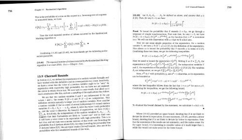
- Page 391: 756 Chapter 13 Randomized Algorithm
- Page 395 and 396: 764 Chapter 13 Randomized Algorithm
- Page 397 and 398: 768 Chapter 13 Randomized Algorithm
- Page 399 and 400: 772 Chapter 13 Randomized Algorithm
- Page 401 and 402: 776 Chapter 13 Randomized Algorithm
- Page 403 and 404: 780 Chapter 13 Randomized Algorithm
- Page 405 and 406: 784 Chapter 13 Randomized Algorithm
- Page 407 and 408: 788 Chapter 13 Randomized Algorithm
- Page 409 and 410: 792 Chapter !3 Randomized Algorithm
- Page 411 and 412: 796 Epilogue: Algorithms That Run F
- Page 413 and 414: 800 Epilogue: Algorithms That Run F
- Page 415 and 416: 8O4 Epilogue: Algorithms That Run F
- Page 417 and 418: 808 References L. R. Ford. Network
- Page 419 and 420: 812 References M. Mitzenmacher and
- Page 421 and 422: 816 Index Approximation algorithms
- Page 423 and 424: 820 Cushions in packet switching, 8
- Page 425 and 426: 824 Index Graphs (cont.) queues and
- Page 427 and 428: 828 Index Mapping genomes, 279, 521
- Page 429 and 430: 832 Index Index 833 Preflow-Push Ma
- Page 431 and 432: 836 Index Stale items in randomized


