Algorithm Design

632
Chapter 11 Approximation Algoriflnns
6
5
2
1
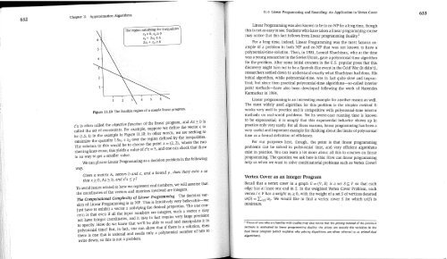
region satisfying the inequalities I
xl>_ 0, x2>- 0
Xl + 2x 2 >_ 6
2xl + x2 >- 6
1 2 4 5 6
Figure 11.10 The feasible region of a simple linear program.
ctx is often called the objective [unction of the linear program, and Ax > b is
called the set of constraints. For example, suppose we define the v~ctor c to
be (1.5, 1) in the example in Figure 11.10; in other words, we are seeking to
minimize the quantity 1.5xl + x2 over the region defined by the inequalities.
The solution to this would be to choose the point x = (2, 2), where the two
slanting lines cross; this yields a value of ctx = 5, and one can check that there
is no way to get a smaller value.
We can phrase Linear Programming as a decision problem in the following
way.
Given a matrix A, vectors b and c, and a bound y, does there, exist x so
that x > O, Ax > b, and ctx < Y ?
To avoid issues related to how we represent real numbers, we will assume that
the coordinates of the vectors and matrices involved are integers.
The Computational Complexity of Linear Programming The decision version
of Linear Programming is in 3ff~. This is intuitively very believable--we
)ust have to exhibit a vector x satisfying the desired properties. The one concern
is that even if all the input numbers are integers, such a vector x may
not have integer coordinates, and it may in fact require very large precision
to specify: How do we know that we’ll be able to read and manipulate it in
polynomial time ?. But, in fact, one can show that if there is a solution, then
there is one that is rational and needs only a polynomial number of bits to
write down; so this is not a problem.
11.6 Linear Programming and Rounding: An Application to Vertex Cover 633
Linear Programming was also known to be in co-2q~P for a long time, though
this is not as easy to see. Students who have taken a linear programming course
may notice that this fact follows from linear programming duality. 2
For a long time, indeed, Linear Programming was the most famous example
of a problem in both N~P and co-~P that was not known to have a
polynomial-time solution. Then, in 1981, Leonid Khachiyan, who at the time
was a young researcher in the Soviet Union, gave a polynomial-time algorithm
for the problem. After some initial concern in the U.S. popular press that this
discovery might ttirn out to be a Sputnik-like event in the Cold War (it didn’t),
researchers settled down to understand exactly what Khachiyan had done. His
initial algorithm, while polynomial-time, was in fact quite slow and impractical;
but since then practical polynomia!-time algorithms--so-called interior
point methods--have also been developed following the work of Narendra
Karmarkar in 1984.
Linear programming is an interesting example for another reason as well.
The most widely used algorithm for this problem is the simplex method. It
works very well in practice and is competitive with polynomial-time interior
methods on real-world problems. Yet its worst-case running time is known
to be exponential; it is simply that this exponential behavior shows up in
practice only very rarely. For all these reasons, linear programming has been a
very useful and important example for thinking about the limits of polynomial
time as a formal definition of efficiency.
For our purposes here, though, the point is that linear programming
problems can be solved in polynomial time, and very efficient algorithms
exist in practice. You can learn a lot more about all this in courses on linear
programming. The question we ask here is this: How can linear programming
help us when we want to solve combinatorial problems such as Vertex Cover?
Vertex Cover as an Integer Program
Recall that a vertex cover in a graph G = (V, E) is a set S _c V so that each
edge has at least one end in S. In the weighted Vertex Cover Problem, each
vertex i ~ V has a weight w i > O, with the weight of a set S of vertices denoted
w(S) = Y~4~s wi. We would like to find a vertex cover S for which w(S) is
minimum.
2 Those of you who are familiar with duality may also notice that the pricing method of the previous
sections is motivated by linear programming duality: the prices are exactly the variables in the
dual linear program (which explains why pricing algorithms are often referred to as primal-dual
algorithms).