You also want an ePaper? Increase the reach of your titles
YUMPU automatically turns print PDFs into web optimized ePapers that Google loves.
Plasma Phys. Control. Fusion 53 (2011) 093001<br />
Topical Review<br />
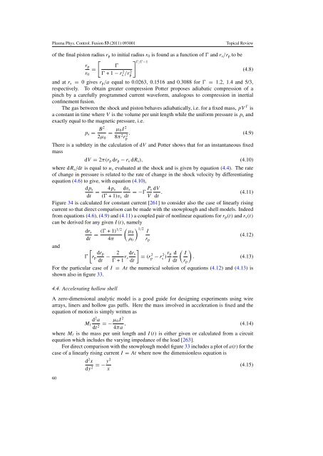
<strong>of</strong> <strong>the</strong> final piston radius r p to initial radius r 0 is found as a function <strong>of</strong> Ɣ and r s /r p to be<br />
[<br />
] Ɣ/Ɣ−1<br />
r p Ɣ<br />
=<br />
(4.8)<br />
r 0 Ɣ +1− rs 2/r2 p<br />
and at r s = 0givesr p /a equal to 0.0263, 0.1516 and 0.3088 for Ɣ = 1.2, 1.4 and 5/3,<br />
respectively. To obtain greater compression Potter proposes adiabatic compression <strong>of</strong> a<br />
<strong>pinch</strong> by a carefully programmed current waveform, analogous to compression in inertial<br />
confinement fusion.<br />
The gas between <strong>the</strong> shock and piston behaves adiabatically, i.e. for a fixed mass, pV Ɣ is<br />
a constant in time where V is <strong>the</strong> volume per unit length while <strong>the</strong> uniform pressure is p s and<br />
exactly equal to <strong>the</strong> magnetic pressure, i.e.<br />
p s = B2<br />
= µ 0I 2<br />
. (4.9)<br />
2µ 0 8π 2 rp<br />
2<br />
There is a subtlety in <strong>the</strong> calculation <strong>of</strong> dV and Potter shows that for an instantaneous fixed<br />
mass<br />
dV = 2π(r p dr p − r s dR s ), (4.10)<br />
where dR s /dt is equal to u s evaluated at <strong>the</strong> shock and is given by equation (4.4). The rate<br />
<strong>of</strong> change in pressure is related to <strong>the</strong> rate <strong>of</strong> change in <strong>the</strong> shock velocity by differentiating<br />
equation (4.6) to give, with equation (4.10),<br />
dp s<br />
= 4p s dv s<br />
=−Ɣ P s dV<br />
dt (Ɣ +1)v s dt V dt . (4.11)<br />
Figure 34 is calculated for constant current [261] to consider also <strong>the</strong> case <strong>of</strong> linearly rising<br />
current so that direct comparison can be made with <strong>the</strong> snowplough and shell models. Indeed<br />
from equations (4.6), (4.9) and (4.11) a coupled pair <strong>of</strong> nonlinear equations for r p (t) and r s (t)<br />
can be derived for any given I(t), namely<br />
( )<br />
dr s (Ɣ 1/2<br />
+1)1/2 µ0 I<br />
= (4.12)<br />
dt 4π ρ 0 r p<br />
and<br />
[<br />
dr p<br />
Ɣ r p − 2 ]<br />
( )<br />
dt Ɣ +1 r dr s<br />
s = (rp 2 dt<br />
− r2 s )r p d I<br />
. (4.13)<br />
I dt r p<br />
For <strong>the</strong> particular case <strong>of</strong> I = At <strong>the</strong> numerical solution <strong>of</strong> equations (4.12) and (4.13) is<br />
shown also in figure 33.<br />
4.4. Accelerating hollow shell<br />
A zero-dimensional analytic model is a good guide for designing experiments using wire<br />
arrays, liners and hollow gas puffs. Here <strong>the</strong> mass involved in acceleration is fixed and <strong>the</strong><br />
equation <strong>of</strong> motion is simply written as<br />
d 2 a<br />
M l<br />
dt =−µ 0I 2<br />
2 4πa , (4.14)<br />
where M l is <strong>the</strong> mass per unit length and I(t) is ei<strong>the</strong>r given or calculated from a circuit<br />
equation which includes <strong>the</strong> varying impedance <strong>of</strong> <strong>the</strong> load [263].<br />
For direct comparison with <strong>the</strong> snowplough model figure 33 includes a plot <strong>of</strong> a(t) for <strong>the</strong><br />
case <strong>of</strong> a linearly rising current I = At where now <strong>the</strong> dimensionless equation is<br />
d 2 x<br />
dy 2 =−y2<br />
(4.15)<br />
x<br />
60


