Elektronika 2010-11.pdf - Instytut Systemów Elektronicznych ...
Elektronika 2010-11.pdf - Instytut Systemów Elektronicznych ...
Elektronika 2010-11.pdf - Instytut Systemów Elektronicznych ...

Create successful ePaper yourself
Turn your PDF publications into a flip-book with our unique Google optimized e-Paper software.
Nevertheless the product of algorithm in such case is numerical<br />
value of<br />
⎛ y<br />
z = arctg 0<br />
, estimated by cumulated sum<br />
⎠ ⎞<br />
n<br />
⎝ x 0<br />
of angles (+/- for left/right) applied for consecutive rotations.<br />
Singular Value Decomposition of a matrix consists in finding<br />
a series of singular values σ 1<br />
, σ 2<br />
..., σ l<br />
which simplify inversion<br />
of matrix. For each matrix M ∈ R m, n there exist orthogonal<br />
matrices U ∈ R m, m and V ∈ R n, n , for which<br />
T<br />
m<br />
,<br />
n<br />
U<br />
MV<br />
= Σ = diag( σ<br />
,σ<br />
K<br />
,σ<br />
)<br />
∈<br />
(5)<br />
1 2<br />
l<br />
R<br />
where l = min(m,n), and for r = rank(A) the diagonal values<br />
fulfill conditions<br />
σ<br />
≥<br />
σ<br />
≥<br />
K<br />
≥<br />
σ<br />
0<br />
(6)<br />
1 2<br />
r<br />
><br />
σ<br />
σ<br />
=<br />
K<br />
=<br />
σ<br />
0<br />
(7)<br />
r<br />
+ 1 = r<br />
+<br />
2<br />
l<br />
=<br />
CORDIC architecture<br />
Two variants of CORDIC architectures are presented in Fig. 1<br />
and 2. Both solutions are full-synchronous with single clock. In<br />
the first – sequential approach, same arithmetic modules are<br />
reused in consecutive iterations. Intermediate results are fed<br />
back via the registers and the appropriate angles are delivered<br />
to arithmetic units by the muxes. Control is provided by iteration<br />
counter. Another concept is pipelined architecture presented in<br />
Fig. 2. Schematic shows a hardware providing 3 consecutive iterations.<br />
Arithmetic blocks are replicated for each iteration, thus<br />
the data flow may form a pipeline. This solution provides much<br />
faster throughput, lower flexibility and needs more hardware resources.<br />
On the other hand the control circuitry is more simple<br />
for this solution, leading to some savings and much higher clo-<br />
nreset<br />
A pseudo-inverse matrix M + may be determined by<br />
<br />
M<br />
+<br />
+<br />
=<br />
V<br />
Σ<br />
U<br />
where Σ + is a pseudo-inverse of diagonal matrix, i.e. it is diagonal<br />
matrix formed by inverted (when non-zero) values of.<br />
SVD is currently classified among the most efficient numerical<br />
methods leading to matrices inversion σ 1<br />
, σ 2<br />
..., σ l<br />
. SVD may be<br />
performed by the appropriate rotation of a matrix. For a basic<br />
2 × 2 matrix M<br />
= ⎡<br />
a<br />
b<br />
⎤ the rotation angle is .<br />
⎣<br />
c<br />
d<br />
⎛ c + b<br />
arctg<br />
⎞<br />
⎦<br />
⎝<br />
d<br />
−<br />
a<br />
⎠<br />
This operation may be done by double use of CORDIC<br />
in two modes. First the appropriate angles are determined<br />
and then the rotations are performed. Due to the properties of<br />
CORDIC the iterations may be described by combinations of<br />
adding/subtracting and shifts of bits:<br />
x<br />
i<br />
+ 1 =<br />
x<br />
i<br />
+<br />
δ<br />
i<br />
⋅<br />
SHIFT i<br />
(<br />
y<br />
i<br />
)<br />
(8)<br />
y<br />
i+ 1 =<br />
y<br />
i<br />
− δ i<br />
⋅<br />
SHIFT i<br />
(<br />
x<br />
i<br />
)<br />
(9)<br />
+<br />
δ<br />
where δ i<br />
= +/-1 denotes left or right shift. Eventually hardware<br />
implementation of CORDIC consists of adders, subtractors<br />
and muxes<br />
T<br />
xin<br />
yin<br />
zin<br />
i<br />
i<br />
i<br />
rotation<br />
angle<br />
clk<br />
nreset<br />
clk<br />
nreset<br />
clk<br />
i<br />
shift<br />
i<br />
shift<br />
i<br />
+1<br />
"0000 "<br />
±<br />
di<br />
±<br />
di<br />
±<br />
di<br />
start, i<br />
Fig. 1. CORDIC – sequential architecture<br />
Rys. 1. Architektura CORDIC w wersji sekwencyjnej<br />
i<br />
i<br />
i<br />
nreset<br />
enable<br />
clk<br />
nreset<br />
enable<br />
clk<br />
nreset<br />
enable<br />
clk<br />
nreset<br />
clk<br />
xout<br />
yout<br />
zout<br />
i<br />
nreset<br />
nreset<br />
nreset<br />
xin<br />
±<br />
±<br />
±<br />
xout<br />
clk<br />
clk<br />
shift >> 1<br />
clk<br />
shift >> 2<br />
d<br />
d<br />
d<br />
nreset<br />
nreset<br />
shift >> 1<br />
nreset<br />
shift >> 2<br />
yin<br />
±<br />
±<br />
±<br />
yout<br />
clk<br />
nreset<br />
d<br />
clk<br />
d<br />
clk<br />
d<br />
zin<br />
nreset<br />
nreset<br />
clk<br />
rotation<br />
angle 1<br />
±<br />
clk<br />
rotation<br />
angle 2<br />
d<br />
d<br />
d<br />
Fig. 2. CORDIC – pipelined architecture Rys. 2. Architektura CORDIC w wersji potokowej<br />
±<br />
clk<br />
rotation<br />
angle 3<br />
±<br />
zout<br />
<strong>Elektronika</strong> 11/<strong>2010</strong> 27