Elektronika 2010-11.pdf - Instytut SystemÃ³w Elektronicznych ...

ok LI nr 11/2010 

• MATERIAŁY • KONSTRUKCJE • UKŁADY 

• SYSTEMY • MIKROELEKTRONIKA 

• OPTOELEKTRONIKA • FOTONIKA 

konstrukcje technologie zastosowania 

MIESIECZNIK NAUKOWO-TECHNICZNY 

• ELEKTRONIKA MIKROFALOWA 

• MECHATRONIKA 

• ENERGOELEKTRONIKA • INFORMATYKA 

ZESPÓŁ REDAKCYJNY 

prof. dr hab. inż. Jerzy Klamka – redaktor naczelny 

Bożena Lachowicz – sekretarz redakcji 

Stali współpracownicy: mgr inż. Wiesław Jabłoński, 

mgr inż. Krzysztof Kowalski, mgr inż. Cezary Rudnicki 

Adres redakcji: ul. Chmielna 6 m.6, 00-020 Warszawa, 

tel./fax (022) 827 38 79; tel.: 826 65 64, 

e-mail: elektronika@red.pl.pl, www.elektronika.orf.pl 

Zamówienia na reklamę przyjmuje redakcja lub Dział Reklamy 

i Marketingu, ul. Mazowiecka 12, 00-950 Warszawa, skr. 1004, 

tel./fax (022) 827 43 66, 826 80 16, e-mail: reklama@sigma-not.pl 

Kolportaż: ul. Ku Wiśle 7, 00-716 Warszawa, tel. (022) 840 35 89; 

tel./fax: (022) 840 59 49, (022) 891 13 74 

RADA PROGRAMOWA 

prof. dr hab. inż. Władysław Torbicz (PAN) – przewodniczący 

prof. dr hab. inż. Leonard Bolc, dr hab. inż. Jerzy Czajkowski, prof. 

dr hab. Zdzisław Drozd, prof. dr hab. inż. Jerzy Frączek, dr hab inż. 

Krzysztof Górecki, dr inż. Józef Gromek, mgr inż. Jan Grzybowski, 

prof. dr hab. Ryszard Jachowicz, prof. dr hab. Włodzimierz 

Janke, prof. dr hab. Włodzimierz Kalita, inż. Stefan Kamiński, prof. 

dr hab. inż. Marian P. Kaźmierkowski, dr inż. Wojciech Kocańda, 

prof. dr hab. Bogdan Kosmowski, mgr inż. Zbigniew Lange, 

dr inż. Zygmunt Łuczyński, prof. dr hab. inż. Józef Modelski, prof. dr 

hab. Tadeusz Morawski, prof. dr hab. Bohdan Mroziewicz, prof. dr hab. 

Andrzej Napieralski, prof. dr hab. Tadeusz Pałko, prof. dr hab. inż. Marian 

Pasko, dr hab. inż. Ryszard Romaniuk, dr hab. inż. Grzegorz Różański, 

prof. dr hab. inż. Edward Sędek, prof. dr hab. Ludwik Spiralski, 

prof. dr hab. inż. Zdzisław Trzaska, mgr inż. Józef Wiechowski, prof. 

dr hab. inż. Marian Wnuk, prof. dr hab. inż. Janusz Zarębski 

Czasopismo dotowane przez Ministerstwo Nauki 

i Szkolnictwa Wyższego. Za opublikowane w nim artykuły 

MNiSzW przyznaje 9 punktów. 

SIGMA - NOT 

Spółka z o.o. 

00-950 Warszawa 

skrytka pocztowa 1004 ul. Ratuszowa 

11 

tel.: (0-22) 818 09 18, 818 98 32 

fax: (022) 619 21 87 

Internet 

http://www.sigma-not.pl 

Prenumerata 

e-mail: kolportaz@sigma-not.pl 

Informacje 

e-mail: informacja@sigma-not.pl 

“Elektronika” jest wydawana 

przy współpracy Komitetu Elektroniki 

i Telekomunikacji Polskiej Akademii Nauk 

IEEE 

WYDAWNICTWO 

CZASOPISM I KSIĄŻEK 

TECHNICZNYCH 

Redakcja współpracuje 

z Polską Sekcją IEEE 

„Elektronika” jest notowana 

w międzynarodowej bazie IEE 

Inspec 

Publikowane artykuły naukowe były 

recenzowane przez samodzielnych 

pracowników nauki 

Redakcja nie ponosi odpowiedzialności 

za treść ogłoszeń. Zastrzega 

sobie prawo do skracania i adiustacji 

nadesłanych materiałów. 

Indeks 35722 

Nakład do 2000 egz. 

Skład i druk: Drukarnia SIGMA-NOT Sp. z o.o. 

Spis treści ● Contents 

Nonlinear compact thermal model of SiC power semiconductor 

devices (Nieliniowy skupiony model termiczny półprzewodnikowych 

elementów mocy wykonanych z węglika krzemu) 

– K. Górecki, J. Zarębski, D. Bisewski, J. Dąbrowski . . . . . . . . . 9 

Krummenacher feedback analysis for high-count-rate semiconductor 

pixel detector readout (Analiza sprzężenia zwrotnego 

Krummenachera pod kątem zastosowania w szybkich 

układach odczytu półprzewodnikowych detektorów mozaikowych) 

– R. Szczygieł . . . . . . . . . . . . . . . . . . . . . . . . . . . . . . . . . 12 

Testing of interconnections with use of reduced-size signature-based 

diagnostic dictionary (Testowanie uszkodzeń 

w połączeniach z wykorzystaniem sygnaturowego słownika 

diagnostycznego o zredukowanym rozmiarze) – T. Garbolino, 

K. Gucwa, A. Hławiczka.. . . . . . . . . . . . . . . . . . . . . . . . . . . . . . . 15 

The Time-over-Threshold based silicon strip detector readout 

(Odczyt do krzemowych detektorów paskowych oparty 

o metodę Time-over-Threshold) – K. Kasiński . . . . . . . . . . . . . 19 

The design of low power 11.6 mW high speed 1.8 Gb/s standalone 

LVDS Driver in 0.18 µm CMOS (Projekt scalonego 

nadajnika standardu LVDS o niskim poborze mocy 11,6 mW 

i 1,8 Gb/s szybkości transmisji danych) – R. Kłeczek . . . . . . . . 23 

CORDIC and SVD implementation in digital hardware (Realizacja 

algorytmów CORDIC i SVD w układzie cyfrowym) – P.M. 

Szecówka, P. Malinowski.. . . . . . . . . . . . . . . . . . . . . . . . . . . . . . 26 

Lab-on-a-chip for developmental competence assessment 

of bovine oocytes (Lab-chip do oceny jakościowej potencjału 

rozwojowego oocytów bydlęcych) – R. Walczak, P. Szczepańska, 

J. Dziuban, B. Kempisty, M. Jackowska, P. Antosik, J. Jaśkowski, 

A. Chełmońska-Soyta . . . . . . . . . . . . . . . . . . . . . . . . . . 30 

Image sensor – based fluorescence detection for lab-on-achip 

(Detekcja fluorescencji w lab-chipach z wykorzystaniem 

czujnika obrazu) – R. Walczak . . . . . . . . . . . . . . . . . . . . . . . . . 33 

Scripting languages for simulations in modern SCADA systems 

(Wykorzystanie języków skryptowych dla symulacji 

w nowoczesnych systemach SCADA) – P. Marciniak, Z. Kulesza, 

A. Napieralski, R. Kotas . . . . . . . . . . . . . . . . . . . . . . . . . . . 36 

FPGA implementation of feature extraction algorithm for 

speaker verification (Implementacja algorytmu estymacji 

cech sygnału mowy systemu automatycznej weryfikacji mówcy 

w układzie FPGA) – M. Staworko, M. Rawski . . . . . . . . . . . . . . 41 

Digital implementation of a programmable type-2 fuzzy logic 

controller (Cyfrowa realizacja programowalnego sterownika 

rozmytego 2-go rzędu) – M. Bryk, A. Wielgus . . . . . . . . . . . . . . 44 

Universal Tool for Estimation of Programmable Logic Controllers 

Processing Power (Uniwersalne narzędzie do szacowania 

mocy obliczeniowej sterowników przemysłowych) 

– Z. Kulesza, S. Marasek . . . . . . . . . . . . . . . . . . . . . . . . . . . . . . 48 

XML markup language based design tool integration method 

in distributed design environments (Metoda integracji narzędzi 

w rozproszonych środowiskach projektowania wykorzystująca 

język znaczników XML) – M. Szlęzak, A. Pawlak, 

K. Wojciechowski . . . . . . . . . . . . . . . . . . . . . . . . . . . . . . . . . . . . 51 

A dedicated high-level language for implementing nonrecursive 

filter banks and transforms (Dedykowany język wysokiego 

poziomu do implementowania nierekursywnych banków 

filtrów i transformacji) – M. Parfieniuk. . . . . . . . . . . . . . . . . . . . . 55 

Elektronika 11/2010

Expandable GSM and GPS systems simulator (Rozbudowany 

symulator systemów GSM oraz GPS) – J. Pochmara, J. Pałasiewicz, 

P. Szablata . . . . . . . . . . . . . . . . . . . . . . . . . . . . . . . . . . 60 

Alvis approach to Hexor robot controller development (Zastosowanie 

języka Alvis do projektowania sterownika dla robota 

Hexor) – M. Szpyrka, P. Matyasik, R. Mrówka . . . . . . . . . . . . 63 

Model of human palm controlled by glove with micromachined 

accelerometers (Model ludzkiej dłoni sterowanej przez 

rękawicę wyposażoną w mikromaszynowe czujniki przyspieszenia) 

– R. Kotas, Z. Kulesza, W. Tylman, A. Napieralski, 

P. Marciniak . . . . . . . . . . . . . . . . . . . . . . . . . . . . . . . . . . . . . . . . 67 

TECHNIKA SENSOROWA: Bezkontaktowy czujnik przemieszczenia 

w złożonym układzie pomiarowym charakterystyk 

elektro-termo-mechanicznych stopów z pamięcią kształtu 

(Non-contact sensor of displacement in complex measurement 

system for measuring the electro-thermo-mechanical characteristics 

of SMA) – G. Kłapyta, M. Kciuk . . . . . . . . . . . . . . . . . . . . 71 

TECHNIKA MIKROFALOWA I RADIOLOKACJA: Poprawa zależności 

poziomu listków bocznych od współczynnika kompresji 

dla sygnałów złożonych z małą bazą (Peak-to-sidelobe 

level vs. time-bandwidth product improvement for complex 

radar signals with small base) – M. Łuszczyk . . . . . . . . . . . . . . 75 

TECHNIKI INFORMATYCZNE: Między Web 2.0 i 3.0: Mobilne 

systemy informacyjne z rozszerzoną rzeczywistością (Between 

Web 2.0 and Web 3.0: Mobile information systems using 

Augmented Reality) – J. Brzostek-Pawłowska . . . . . . . . . . . . . 79 

Using multi-frequency coherent signal to measurement of frequency 

response of narrow-band LF and HF circuits (Zastosowanie 

wieloczęstotliwościowego sygnału koherentnego 

do pomiaru charakterystyk częstotliwościowych układów wąskopasmowych 

m.cz. oraz w.cz.) – J. Duchiewicz, A.S. Sowa, 

J.S. Witkowski, A. Francik, A.L. Dobrucki, B. Idźkowski . . . . . . . 88 

Radiokomunikacyjne aspekty planu implementacji strategii 

e-nawigacji (Radiocommunication aspects of an e-navigation 

strategy implementation plan) – K. Korcz. . . . . . . . . . . . . . . . . . 92 

Urządzenie do generacji silnych i ultrasilnych pól magnetycznych 

oraz sprzężony z nim układ pomiarowy (Device for the 

generation of strong and ultrastrong magnetic fields with the 

measuring system) – D. Płoch, P. Sliż, E. Szeregij . . . . . . . . . . . 97 

Aspekty algorytmiczne organizacji jednostki procesorowej 

do mnożenia liczb Cayleya ( Algorithmic aspects of Cayley 

numbers multiplier organization) – A. Tariov, G. Tariova . . . . . 104 

TECHNIKA PRÓŻNI I TECHNOLOGIE PRÓŻNIOWE: Biuletyn 

Polskiego Towarzystwa Próżniowego 1 (50) 2010. . . . . . . . 109 

Spektrometr Elektronowego Rezonansu Paramagnetycznego 

(EPR), umożliwiający ilościowe pomiary liczby spinów 

w badanej próbce (Electron Paramagnetic Resonance (EPR) 

spectrometer for quantitative measurements of the spins number 

in the sample under test) – J. Duchiewicz, A. Dobrucki, 

A. Francik, W. Stachowicz, T. Oleś, T. Duchiewicz . . . . . . . . . . 117 

Moduły lokalizacji oraz testy chipów GNSS dla elementów systemu 

PROTEUS (The location modules and tests of GNSS receivers 

for the elements of PROTEUS system) – R. Darakchiev, 

P. Sitek, K. Brzostowski, A. Foks-Ryznar, M. Kalarus, R. Zdunek . .122 

Analiza możliwości zastosowania sensorów inercjalnych 

MEMS w projekcie PROTEUS (An analysis of the applicability 

of MEMS inertial sensors in the PROTEUS project) – M. Kalarus, 

P. Sitek, K. Brzostowski, A. Foks-Ryznar, R. Darakchiev . 127 

Antena mikropaskowa o poszerzonym paśmie pracy (Broadband 

microstrip patch antenna) – M. Pergoł, W. Zieniutycz, Ł. 

Sorokosz . . . . . . . . . . . . . . . . . . . . . . . . . . . . . . . . . . . . . . . . . 130 

Properties of feature contours for audio classification tasks 

(Właściwości konturów cech w zadaniach klasyfikacji sygnałów 

akustycznych) – T. Mąka . . . . . . . . . . . . . . . . . . . . . . . . . . . . . 134 

Streszczenia artykułów ● Summaries of the articles 

GÓRECKI K., ZARĘBSKI J., BISEWSKI D., DĄBROWSKI J.: Nieliniowy 

skupiony model termiczny półprzewodnikowych elementów mocy 

wykonanych z węglika krzemu 

Elektronika (LI), nr 11/2010, s. 9 

W pracy przedstawiono nieliniowy skupiony model termiczny 

półprzewodnikowych elementów mocy wykonanych z węglika krzemu, 

sformułowany na bazie sieci Cauera. Zaprezentowano opis analityczny 

modelu oraz metodę wyznaczania wartości parametrów tego modelu. 

Dokładność i przydatność zaproponowanego modelu zweryfikowano 

doświadczalnie dla diody Schottky’ego i tranzystora MESFET przy różnych 

warunkach chłodzenia tych elementów. 

Słowa kluczowe: model termiczny, węglik krzemu, półprzewodnikowe 

elementy mocy 

SZCZYGIEŁ R.: Analiza sprzężenia zwrotnego Krummenachera pod 

kątem zastosowania w szybkich układach odczytu półprzewodnikowych 

detektorów mozaikowych 


Obwód sprzężenia zwrotnego Krummenachera [1] jest często używany 

we wzmacniaczach ładunkowych podłączonych do detektorów półprzewodnikowych 

ze sprzężeniem DC. Układ ten w bardzo prostej strukturze 

zapewnia podwójną funkcjonalność: ciągłe kasowanie wzmacniacza ładunkowego 

i kompensację prądu upływu detektora. Pomimo prostej budowy 

analiza tego układu pod kątem szybkości działania jest dosyć złożona. 

Przedstawiony artykuł prezentuje analizę niniejszego obwodu w oparciu 

o parametry technologii 90 nm CMOS ukierunkowaną na aplikacje do 

odczytu półprzewodnikowych detektorów hybrydowych realizowanych 

w technologiach submikronowych lub 3D. 

Słowa kluczowe: sprzężenie Krummenachera, CSA, detektor mozaikowy 

GÓRECKI K., ZARĘBSKI J., BISEWSKI D., DĄBROWSKI J.: Nonlinear 

compact thermal model of SiC power semiconductor devices 

Elektronika (LI), no 11/2010, p. 9 

The paper deals with the nonlinear compact thermal model of SiC power 

semiconductor devices, based on the Cauer network. The analytical description 

of the model and the method of the model parameter estimation 

are presented. The accuracy and usefulness of the model is verified experimentally 

for the Schottky diode and MESFET transistor at their various 

cooling conditions. 

Keywords: Thermal model, silicon carbide, power swmiconductor devices 

SZCZYGIEŁ R.: Krummenacher feedback analysis for high-countrate 

semiconductor pixel detector readout 


The Krummenacher feedback circuit [1] is a well know and often used in 

charge sensitive amplifiers (CSA) connected to DC-coupled semiconductor 

detectors. The circuit provides in a very simple structure dual functionality: 

continuous reset and detector leakage current compensation. In spite 

of the simplicity the characterization of the circuit for high speed applications 

is not very straightforward. This article presents an analysis of the 

feedback circuit based on 90 nm CMOS and technology and targeted at 

high-count-rate semiconductor hybrid pixel detector applications realized 

in submicron or 3D technologies. 

Keywords: Krummenacher feedback, CSA, pixel detector 

 



GARBOLINO T., GUCWA K., HŁAWICZKA A.: Testowanie uszkodzeń 

w połączeniach z wykorzystaniem sygnaturowego słownika diagnostycznego 

o zredukowanym rozmiarze 


W artykule zaproponowano nową metodę redukcji rozmiaru syganturowego 

słownika diagnostycznego, który jest wykorzystywany do testownia uszkodzeń 

statycznych i opóźnieniowych w połączeniach testowanych przez 

rejestr pierścieniowy R-LFSR. Nowo opracowana metoda – podobnie jak 

w poprzednich pracach autorów – zakłada, że testowana magistrala n‐bitowa 

zostaje podzielona na b jednakowych fragmentów o szerokości k bitów 

każdy. Każdy taki fragment magistrali jest testowany przez oddzielny rejestr 

R-LFSR złożony z 2k przerzutników D. Procedura testowa obejmuje cztery 

fazy, w czasie których rejestry parzyste i nieparzyste pracują naprzemiennie. 

Takie podejście eliminuje zjawisko wzajemnego wpływu na siebie sąsiednich 

rejestrów R-LFSR, które było wadą poprzednich rozwiązań ponieważ ograniczało 

możliwość zmniejszenia rozmiaru słownika diagnostycznego. Nowa 

technika umożliwia detekcję, lokalizację oraz identyfikację wszystkich zamodelowanych 

uszkodzeń, mogących wystapić na n‐bitowej magistrali, oraz wymaga 

słownika diagnostycznego o znacznie mniejszym rozmiarze. Rozmiar 

tego słownika jest określony wyłącznie przez krotność uszkodzeń r w każdym 

k‐bitowym fragmencie magistrali, nawet gdy szerokość tej magistrali n >>k. 

Słowa kluczowe: testowanie połączeń; wbudowane samotestowanie; rejestr 

pierścieniowy; sygnatura; sygnaturowy słownik diagnostyczny 

KASIŃSKI K.: Odczyt do krzemowych detektorów paskowych oparty 

o metodę Time-over-Threshold 


Praca przedstawia project układu odczytowego dla krzemowych detektorów 

paskowych. Układ może znaleźć zastosowanie w wielokanałowych 

specjalizowanych układach scalonych dla potrzeb eksperymentów Fizyki 

Wysokich Energii. Pomiar ładunku jest oparty o metodę Time-over-Threshold 

pozwalającej na integrację niskomocowego przetwornika Analogowo- 

Cyfrowego w każdym kanale. 

Słowa kluczowe: wielokanałowy układ scalony, krzemowy detektor paskowy, 

Time-over-Threshold 

KŁECZEK R.: Projekt scalonego nadajnika standardu LVDS o niskim 

poborze mocy 11,6 mW i 1,8 Gb/s szybkości transmisji danych 


Niskonapięciowa transmisja różnicowa LVDS dzięki swoim licznym zaletom 

jest coraz częściej stosowana w układach transmisji danych. Praca 

przedstawia projekt modułu układu scalonego nadajnika LVDS. Układ 

został zaprojektowany w technologii CMOS firmy United Microelectronics 

Corporation, o rozmiarze charakterystycznym równym 180 nm. Opracowane 

rozwiązanie nadajnika jest kompatybilne ze specyfikacją IEEE. Zaprojektowany 

nadajnik LVDS charakteryzuje się bardzo niskim poziomem 

statycznego 7,5 mW, dynamicznego zużycia mocy 8,5 mW (11,6 mW), 

podczas transmisji danych z szybkością 400 Mb/s (1,8 Gb/s). 

Słowa kluczowe: niskonapięciowa transmisja różnicowa LVDS, transmisja 

danych, układy wejścia/wyjścia, układ scalony, technologia CMOS, 

system transmisyjny, przepustowość danych 

SZECÓWKA P.M., MALINOWSKI P.: Realizacja algorytmów CORDIC 

i SVD w układzie cyfrowym 


Algorytm SVD (Singular Value Decomposition) jest zaliczany do najbardziej 

efektywnych metod pozwalających odwracać macierze. Artykuł opisuje próbę 

sprzętowej realizacji algorytmów CORDIC i SVD. Rozważono szereg 

architektur – warianty bardzo oszczędne sekwencyjne, a także rozwiązania 

pozwalające uzyskać wysoką wydajność obliczeniową, z przetwarzaniem 

potokowym. Porównano także rezultaty uzyskane przy zastosowaniu arytmetyki 

stało- i zmiennoprzecinkowej. Koncepcje zostały zaimplementowane 

w języku opisu sprzętu (VHDL) poddane weryfikacji i syntezie za pomocą 

narzędzi XIlinx. Niektóre warianty zostały przetestowane fizycznie. 

Słowa kluczowe: CORDIC, SVD, układ cyfrowy, VHDL, układ FPGA 

WALCZAK R., SZCZEPAŃSKA P., DZIUBAN J., KEMPISTY B., JACKOW- 

SKA M., ANTOSIK P., JAŚKOWSKI J., CHEŁMOŃSKA-SOYTA A.: Labchip 

do oceny jakościowej potencjału rozwojowego oocytów bydlęcych 


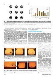
W artykule przedstawiono nowa spektrofotometryczną metodę wykorzystującą 

mikrosystem typu lab-on-a-chip do jakościowej oceny oocytów 

bydlęcych. Przedstawiono wyniki badań z rzeczywistym materiałem biologicznym. 

Otrzymano zgodność pomiędzy wynikami uzyskanymi za pomocą 

opisanego systemu a metodą referencyjną. 

Słowa kluczowe: lab-on-a-chip, bydło, oocyt, zarodek, kompetencje rozwojowe 

GARBOLINO T., GUCWA K., HŁAWICZKA A.: Testing of interconnections 

with use of reduced-size signature-based diagnostic dictionary 


The paper presents a new method for size reduction of a signature-based 

diagnostic dictionary that is normally used for testing of static and delay 

faults in interconnections that are tested by means of an R-LFSR ring 

register. The newly developed method, similarly to the previous studies 

of the authors, assume that the n-bit bus under test is split into b fragments 

with their width of k bits each. Each fragment of the bus is tested with use 

of a separate 2k-bit R‐LFSR. The test procedure consists of four phases 

during which odd and even registers operate alternately. Such an approach 

eliminates effect of mutual impact between states of neighbouring 

R-LFSRs in case of shorts between feedback lines of these registers. These 

possible interactions were a drawback of previous solutions as they 

limited the possibility to reduce size of the diagnostic dictionary. Owing to 

application of this new technique to full detection, localization and identification 

of all the considered faults that may occur on an n-bit bus, the new 

solution needs much smaller dictionary, where its size is determined by 

the multiplicity r of faults within each k-bit fragment, even if the bus width 

n >> k. 

Keywords: interconnect test; BIST; interconnect BIST; IBIST; ring LFSR; 

signature; diagnostic dictionary 

KASIŃSKI K.: The Time-over-Threshold based silicon strip detector 

readout 


This work presents the project of a silicon strip detector readout circuit. 

The circuit is to be used in the multi-channel detector readout integrated 

circuit with a possible application in High Energy Physics experiments. The 

charge measurement is based on the Time-over-Threshold method which 

allows integration of the low-power ADC into each channel. 

Keywords: integrated cicuit, silicon strip detector, Time-over-Threshold, 

multichannel 

KŁECZEK R.: The design of low power 11.6 mW high speed 1.8 Gb/s 

stand-alone LVDS Driver in 0.18 µm CMOS 


Due to many advantages low voltage differential signaling LVDS has become 

a popular choice for fast data on-chip transmission, on-board/backplane or 

cable connections. LVDS standard offers achieving a high-speed data transmission 

and low power consumption at the same time. This paper presents 

a description of standard and design of LVDS transmitter fully compatible with 

IEEE specification, implemented in CMOS 180 nm UMC technology. The main 

driver’s functional blocks: LVDS core and common mode feedback (CMFB) 

are described in detail, whereas control buffer and band-gap reference source 

are only mentioned. Results of simulation are also presented. Designed LVDS 

driver characterizes a very low level of static 7.5 mW and dynamic 8.5 mW 

(11.6 mW) power dissipation at data rate 400 Mb/s (1.8 Gbp/s). 

Keywords: low-voltage differential signaling LVDS, fast data communications 

circuits, high speed integrated circuits (IC), input/output (I/O) drivers, 

low power design 

SZECÓWKA P.M., MALINOWSKI P.: CORDIC and SVD implementation 

in digital hardware 


Singular Value Decomposition (SVD) is classified among the most effective 

numeric methods of matrices inversion. The paper presents a study of 

hardware implementation of SVD and CORDIC algorithms. Various digital 

architectures were proposed and compared, including low-cost sequential 

and high-performance pipelined solutions. Fixed point and floating point 

arithmetic was considered. The concepts were implemented in VHDL, verified 

and synthesized with Xilinx tools. Selected approach was physically 

implemented and tested. 

Keywords: CORDIC, SVD, digital, hardware, VHDL, FPGA 

WALCZAK R., SZCZEPAŃSKA P., DZIUBAN J., KEMPISTY B., JACKOW- 

SKA M., ANTOSIK P., JAŚKOWSKI J., CHEŁMOŃSKA-SOYTA A.: Lab-ona-chip 

for developmental competence assessment of bovine oocytes 


In the paper a novel spectrophotometric methodology utilizing lab-on-achip 

device for assessment of quality of bovine oocytes is presented. Qualification 

results of living bovine oocytes are described. Good correlation of 

obtained results with reference methodology has been achieved. 

Keywords: lab-on-a-chip, bovine, oocyte, embryo, development competence 



WALCZAK R.: Detekcja fluorescencji w lab-chipach z wykorzystaniem 

czujnika obrazu 


W artykule przedstawiono krótką dyskusję na temat detekcji fluorescencji 

w mikrosystemach typu lab-on-a-chip. Przedstawiono nowe rozwiązanie 

technicznye bazujace na czujniku obrazowym współpracującym ze specjalizowanych 

oprogramowaniem autorskim. Przedstawiono przykład 

wykorzystujący opracowany układ detekcji fluorescencji w przenośnym 

urządzeniu do detekcji patogenów żywności wykorzystujący analizę DNA 

bakterii. 

Słowa kluczowe: detekcja fluorescencji, mikrofluidyka, lab-on-a-chip 

MARCINIAK P., KULESZA Z., NAPIERALSKI A., KOTAS R.: Wykorzystanie 

języków skryptowych dla symulacji w nowoczesnych systemach 

SCADA 


Głównym celem napisania tego artykułu jest zaprezentowanie nowoczesnych 

możliwości systemów SCADA (Supervisory Control And Data Acquisition). 

Pierwsza część skupia się na historii powstawania systemów 

SCADA i ukazuje, jak zmieniają się one od momentu ich pojawienia się.. 

Zawiera także opis języków skryptowych, które są wbudowane w oprogramowanie 

SCADA. Druga część artykułu prezentuje zdolność wykorzystania 

języków skryptowych na przykładzie Visual Basic for Applications, 

który jest zintegrowany z oprogramowaniem iFIX Intellution HMI/SCADA 

Automation Software. Wszystkie przykłady zaczerpnięte są z pracy magisterskiej 

autora pod tytułem „Wykorzystanie pakietów SCADA w wizualizacji 

procesu produkcji leków”, której głównym celem było wykonanie 

systemu wizualizacji. System ten prezentuje realny proces produkcji, który 

jest wdrożony w jednej z firm farmaceutycznych w Łodzi. 

Słowa kluczowe: system SCADA, język skryptowy, archiwizacja danych, 

interfejs użytkownika 

STAWORKO M., RAWSKI M.: Implementacja algorytmu estymacji 

cech sygnału mowy systemu automatycznej weryfikacji mówcy w 

układzie FPGA 


Artykuł przedstawia układ estymacji cech sygnału mowy w systemie automatycznej 

weryfikacji mówcy bazujący na parametrach LFCC z wykorzystaniem 

nowej architektury realizującej proces uśredniania w dziedzinie 

częstotliwości. Proponowane rozwiązanie jest przeznaczone do implementacji 

w strukturach reprogramowalnych jako część systemu jednoukładowego, 

charakteryzuje się niskim poborem mocy oraz krótkim czasem 

wyznaczania parametrów LFCC z sygnału mowy. 

Słowa kluczowe: automatyczna weryfikacja mówcy, LFCC, FPGA, niski 

pobór mocy 

BRYK M., WIELGUS A.: Cyfrowa realizacja programowalnego sterownika 

rozmytego 2-go rzędu 


W artykule przedstawiono projekt cyfrowego układu scalonego CMOS realizującego 

sterownik rozmyty 2-go rzędu. Zaproponowana architektura 

układu umożliwia połączenie sekwencyjnego przetwarzania kolejnych reguł 

rozmytych z równoległym przetwarzaniem dla górnej i dolnej funkcji 

przynależności każdego zbioru rozmytego. Uzyskany sparametryzowany 

model VHDL umożliwia syntezę układu o rozmiarze wymaganym w konkretnej 

realizacji. 

Słowa kluczowe: zbiór rozmyty II rzędu; sterownik rozmyty, realizacja 

cyfrowa 

KULESZA Z., MARASEK S.: Uniwersalne narzędzie do szacowania 

mocy obliczeniowej sterowników przemysłowych 


Artykuł omawia problematykę metod szacowania mocy obliczeniowej sterowników 

przemysłowych. Ze względu na brak uniwersalnych metod konieczne 

było opracowanie dedykowanego benchmarka syntetycznego. Poprzez symulację 

reprezentatywnego obciążenia programowego został on wykorzystany do 

przetestowania szerokiego zakresu sterowników przemysłowych. Dodatkowe 

testy przeprowadzono w celu zweryfikowania osiągów sterowników dla różnych 

elementów programowych. Otrzymane wyniki zestawiono z istniejącymi 

wyznacznikami mocy obliczeniowej sterowników, wykazując poważne wady 

tych ostatnich. Zaprojektowany benchmark wykazuje cechy prawidłowego 

i uniwersalnego narzędzia do porównywania mocy obliczeniowej sterowników, 

z szansą na praktyczne wykorzystanie w przemyśle. 

Słowa kluczowe: PLC, sterownik, testowanie, benchmarking, moc obliczeniowa 

WALCZAK R.: Image sensor – based fluorescence detection for labon-a-chip 


In the paper a brief discussion on fluorescence detection in lab-on-a-chip 

is carried out. A novel, low-cost image sensor – based detection instrumentation 

co-working with a “clever” software is described. An example of 

application of the novel method in a portable device for detection of food 

pathogens by DNAanalyze is presented. 

Keywords: fluorescence detection, microfluidics, lab-on-a-chip 

MARCINIAK P., KULESZA Z., NAPIERALSKI A., KOTAS R.: Scripting 

languages for simulations in modern SCADA systems 

Elektronika (LI_), no 11/2010, p. 36 

The goal of this research is to present modern SCADA (supervisory control 

and data acquisition) systems abilities. The first part of this article concentrates 

on the SCADA history and shows how SCADA systems have changed 

since they appeared. This part also includes the description of scripting 

languages which are embedded in SCADA software. The second part 

of this research presents scripting languages abilities based on example 

of Visual Basic for Applications which are integrated with iFIX Intellution 

HMI/SCADA Automation Software. All examples come from the author’s 

master thesis which is entitled “The use of SCADA System in Visualization 

of Medicine Production Process”. The main point of this master thesis was 

to create a visualization system. This system presents a real production 

process which is implemented in one of the pharmaceutical companies 

in Lodz. 

Keywords: SCADA system, scripting language, data aquisition, Human 

Machine Interface 

STAWORKO M., RAWSKI M.: FPGA implementation of feature extraction 

algorithm for speaker verification 


In this paper we propose a feature extraction circuit of automatic speaker 

verification system based on the LFCC with novel architecture for spectral 

averaging. Proposed solution is optimized for implementation in programmable 

structures as System on Programmable Chip and significantly reduces 

feature extraction execution time and power consumption. 

Keywords: Terms-automatic speaker verification; LFCC; FPGA; low power 

application 

BRYK M., WIELGUS A.: Digital implementation of a programmable 

type-2 fuzzy logic controller 


This paper presents the design of a digital CMOS integrated circuit implementing 

a type-2 fuzzy logic controller. The proposed architecture is suitable 

for serial processing of fuzzy rules combined with parallel processing 

of upper and lower membership functions of type-2 fuzzy sets. The parameterized 

VHDL model allows to synthesize the circuit of the required size 

for a particular application. Moreover, on-chip programming is performed. 

Keywords: type-2 fuzzy set; fuzzy logic controller; digital implementation 

KULESZA Z., MARASEK S.: Universal Tool for Estimation of Programmable 

Logic Controllers Processing Power 


Article covers the issue of PLC processing power estimation techniques. 

Absence of universal methods entailed need to elaborate specialized 

synthetic benchmark. By simulating representative workload, it was used 

to test wide spectrum of controllers. Additional tests were carried out to 

measure controllers performance for different program items. Obtained 

results are confronted with existing determinants of PLC processing power. 

Serious drawbacks of the latter are shown. On the contrary, designed 

benchmark proves to be appropriate and universal tool for PLC performance 

comparison with promising future applications in industry. 

Keywords: PLC, controller, testing, benchmarking, processing power 

 



SZLĘZAK M., PAWLAK A., WOJCIECHOWSKI K.: Metoda integracji 

narzędzi w rozproszonych środowiskach projektowania wykorzystująca 

język znaczników XML 


Integracja narzędzi projektowania jest zasadniczym problemem w rozproszonym 

projektowaniu układów elektronicznych typu SoC. Artykuł prezentuje 

metody i narzędzia dla opartej o język znaczników XML integracji rozproszonych 

narzędzi.. Pokazano jak XML umożliwia: uniwersalny opis narzędzi, 

łatwe magazynowanie, wyszukiwanie i dostęp do opisów narzędzi, jak 

również zdalne wywoływanie narzędzi. Zaprezentowane koncepcje i metody 

zostały zweryfikowane w środowisku projektowania wykorzystującym narzędzie 

TRMS (ang. Tools Registration and Management Services). Środowisko 

to zawiera, m.in. narzędzie do śledzenia zmian w specyfikacjach dostępnych 

w sieci Internet narzędzi projektowania oraz system ontologiczny, który 

umożliwia wnioskowanie o relacjach pomiędzy zadaniami projektowymi 

a narzędziami. We wnioskach wskazano na zalety wykorzystania języka 

znaczników XML w procesie integracji narzędzi. 

Słowa kluczowe: projektowanie systemów typu SoC, projektowanie 

rozproszone, integracja rozproszonych narzędzi, opis narzędzi w języku 

XML, zarządzanie narzędziami, ontologie dla narządzi projektowania 

PARFIENIUK M.: Dedykowany język wysokiego poziomu do implementowania 

nierekursywnych banków filtrów i transformacji 


W artykule przedstawiono nowatorskie podejście do implementowania nierekursywnych 

banków filtrów i transformacji. Opracowany został dziedzinowy 

język, który pozwala opisywać te systemy przejrzyściej, zwięźlej i szybciej 

niż z użyciem MATLAB/Simulink lub SPL, istniejących narzędzi do rozwijania 

algorytmów cyfrowego przetwarzania sygnałów. Jego składnia jest ukierunkowana 

na ścisłe powiązanie kodu z grafem przepływu danych w rozpatrywanej 

transformacji i na umożliwienie wyspecyfikowania algorytmu w kategoriach 

transformacji elementarnych: obrotów planarnych, odbić, stopni „lifting”, opóźnień 

itp. W odróżnieniu od wymienionych platform, proponowane podejście 

pozwala uniknąć konstruowania skomplikowanych wyrażeń macierzowych, 

choć notacja macierzowa jest dostępna jako podzbiór języka MATLAB. Skojarzony 

kompilator przekształca opisy systemów w dosyć wydajne implementacje 

Java, C++ lub C, które mogą być wykorzystywane do szybkiego 

prototypowania aplikacji, które opierają się na podpasmowej dekompozycji 

sygnałów, lub do przygotowywania funkcji celu na potrzeby optymalizacji 

współczynników schematów obliczeniowych. 

Słowa kluczowe: język dziedzinowy, DSL, kompilator, generacja kodu, 

implementacja, bank/zespół filtrów, transformacja, cyfrowe przetwarzanie 

sygnałów, DSP 

POCHMARA J., PAŁASIEWICZ J., SZABLATA P.: Rozbudowany symulator 

systemów GSM oraz GPS 


Publikacja prezentuje propozycję implementacji prostego symulatora systemów 

GPS i GSM. Moduł został przystosowany do instalacji rozszerzeń zapewniających 

dodatkową funkcjonalność. Urządzenie pozwala na praktyczne 

wykorzystanie przewagi technologii bezprzewodowej w wielu złożonych 

zastosowaniach. Połączenie protokołu NMEA oraz języka komend AT sprawiło, 

że prezentowany system jest kompatybilny z najnowszymi standardami 

obowiązującymi w branży telekomunikacyjnej. Projekt generuje efekty 

spotykane w wysoko-budżetowych rozwiązaniach korzystając z podzespołów 

oferowanych w dostępnych cenach. Dzięki wykorzystaniu popularnego 

standardu krótkich wiadomości (SMS) oraz światowego systemu nawigacji 

(GPS), prezentowany moduł może zostać użyty w każdym projekcie, który 

wykorzystuje powyższe technologie. System może służyć do symulowania 

zachowań telefonu komórkowego, śledzenia innych urządzeń, lokalizowania 

nadajników i prezentowania otrzymanych danych na dowolnej mapie. 

Projekt sprawdzi się również w złożonych procesach obliczeniowych. 

Słowa kluczowe: GSM, GPS, GPRS, NMEA, standard AT, komendy AT, SMS, 

szerokość geograficzna, długość geograficzna, urządzenia śledzące, nadajniki 

SZPYRKA M., MATYASIK P., MRÓWKA R.: Zastosowanie języka Alvis 

do projektowania sterownika dla robota Hexor 


Alvis jest językiem modelowania, rozwijanym głównie z myślą o projektowaniu 

i weryfikacji systemów wbudowanych. Wywodzi się on z algebr procesów CCS 

i XCCS, ale w języku tym równania algebraiczne zostały zastąpione przez język 

programowania wysokiego poziomu oparty na języku Haskell. W przeciwieństwie 

do algebr procesów, które umożliwiają wyłącznie tekstowy opis systemów 

wbudowanych, w języku Alvis struktura projektowanego systemu, z punktu widzenia 

przepływu danych i sterowania, przedstawiana jest graficznie za pomocą 

diagramów komunikacji. Poniższy artykuł zawiera wprowadzenie do języka 

Alvis zilustrowane modelem sterownika dla robota mobilnego Hexor II. 

Słowa kluczowe: język modelowania Alvis, systemy wbudowane, Hexor 

II, modelowanie formalne 

SZLĘZAK M., PAWLAK A., WOJCIECHOWSKI K.: XML markup language 

based design tool integration method in distributed design 

environments 


Design tools integration is a key problem in distributed design of Systemson-Chip. 

The paper presents methods and tools for integration of distributed 

design tools based on the markup language XML which supports 

universal description of tools, straightforward storage, search and retrieval 

of tool descriptions, as well as remote invocation of tools. Presented concepts 

and methods have been verified with the design environment based 

on Tools Registration and Management Services (TRMS). The TRMSbased 

environment includes a tool for Internet-wide tracking of changes 

in design tool specifications and ontology for reasoning on relationships 

between design tasks and tools. Advantages of the approach have been 

summarized. 

Keywords: SoC design, distributed collaborative design; remote tools integration; 

XML-based tool wrapping; tools management; tools ontology 

PARFIENIUK M.: A dedicated high-level language for implementing 

nonrecursive filter banks and transforms 


This paper presents a novel approach to implementing nonrecursive filter 

banks and transforms. A domain-specific language has been developed 

that allows such systems to be described more clearly, more compactly, 

and faster than with either MATLAB/Simulink or SPL, the existing tools for 

developing DSP algorithms. Its syntax is aimed at closely linking code to 

the signal flow graph of a given transform and at allowing the algorithm to 

be specified in terms of elementary transformations: plane rotations, reflections, 

lifting steps, delays, etc. Unlike the mentioned platforms, our approach 

allows to avoid constructing complicated matrix expressions, even 

though matrix notation is supported via a subset of the MATLAB language. 

The associated compiler converts system descriptions into quite efficient 

Java, C++, or C implementations, which can be used to rapidly prototype 

applications based on subband processing of signals or to prepare objective 

functions for optimizing coefficients of computational schemes. 

Keywords: domain-specific language, DSL, compiler, code generation, 

implementation, filter bank, transform, digital signal processing, DSP 

POCHMARA J., PAŁASIEWICZ J., SZABLATA P.: Expandable GSM 

and GPS systems simulator 

Elektrponika (LI), no 11/2010, p. 60 

This paper proposes and implements a simple extendable GSM and GPS 

systems simulator. It allows user to learn advantages of modern wireless 

technology and use it in many complicated solutions. By combining NMEA 

protocol and AT commands, system is compatible with newest standards 

in telecommunication industry. Project uses low cost hardware to produce 

effects that are nowadays only seen in very expensive solutions. By utilizing 

popular short messages standard (SMS) with worldwide working GPS 

system, it is possible to make use of presented module in any project 

involving wireless technology. This system is useful for simulating mobile 

phone, tracking device, localizing beacon within map range and using 

module for more complex data calculating processes. 

Keywords: GSM, GPS, GPRS, NMEA, AT standard, AT commands, SMS, 

latitude, longitude, computer application, tracking device 

SZPYRKA M., MATYASIK P., MRÓWKA R.: Alvis approach to Hexor 

robot controller development 


Alvis is a novel modelling language defined especially for the embedded 

systems design and verification. The language has its origin in CCS and 

XCCS process algebras, but algebraic equations have been replaced with 

a Haskell based high level programming language. Moreover, Alvis provides 

communication diagrams for the visual modelling of an embedded 

system structure, especially from the control and data-flow point of view. 

This paper presents an introduction to Alvis based on a model of a controller 

for the Hexor II mobile robot. 

Keywords: Alvis modelling language, embedded systems, Hexor II Robot, 

formal modelling 



KOTAS R., KULESZA Z., TYLMAN W., NAPIERALSKI A., MARCI- 

NIAK P.: Model ludzkiej dłoni sterowanej przez rękawicę wyposażoną 

w mikromaszynowe czujniki przyspieszenia 


Celem badań zaprezentowanych w artykule było sprawdzenie możliwości 

konstrukcji w pełni niezależnego systemu mikroprocesorowego do wykrywania 

ułożenia ludzkiej dłoni przy wykorzystaniu mikromaszynowych czujników 

przyspieszenia. Zaimplementowany algorytm polega na pomiarze 

przyspieszenia grawitacyjnego. Zaprojektowany system mikroprocesorowy 

analizuje dane z czujników i steruje modelem ludzkiej dłoni wykonanym 

w naturalnej skali. Model składa się z nieruchomego nadgarstka, dwóch 

palców oraz przeciwstawnego kciuka. Każdy palec posiada trzy stopnie 

swobody. Dodatkowy stopień swobody zastosowano dla kciuka. 

Słowa kluczowe: model ludzkiej dłoni, mikromaszynowe czujniki przyspieszenia 

KOTAS R., KULESZA Z., TYLMAN W., NAPIERALSKI A., MARCI- 

NIAK P.: Model of human palm controlled by glove with micromachined 

accelerometers 


The aim of the research presented in this paper was to test the possibility 

of inventing a fully autonomous device to detect the position of the fingers 

with the use of micromachined accelerometers. An implemented algorithm 

is based on the measurement of gravity acceleration. Designed microprocessor 

system analyses that data and controls the model of a human palm 

made in a 1:1 scale. The model has a motionless wrist, two fingers and 

an opposing thumb. Every finger has three joints. An extra joint is made 

for the thumb. This paper is based on the author’s master thesis which is 

entitled “Data glove controlled by a microprocessor system”. 

Keywords: model of human palm, micromachined accelerometers 

KŁAPYTA G., KCIUK M.: Bezkontaktowy czujnik przemieszczenia 

w złożonym układzie pomiarowym charakterystyk elektro-termo-mechanicznych 

stopów z pamięcią kształtu 


Artykuł przedstawia koncepcję oraz opis realizacji praktycznej bezkontaktowego 

czujnika przemieszczenia, pracującego synchronicznie jako element 

złożonego systemu pomiarowego, służącego do wyznaczania charakterystyk 

elektro-termo-mechanicznych aktuatorów ze stopów z pamięcią 

kształtu. Odkształcenie cięgna jest mierzone za pomocą dwukierunkowego, 

scalonego, optycznego licznika impulsów. Pomiar odkształcenia jest 

realizowany synchronicznie z pomiarem innych wielkości – elektrycznych 

(prąd, napięcie) oraz nieelektrycznych (temperatura). Wartość odkształcenia 

aktuatora zamieniana jest na sygnał PWMo wypełnieniu proporcjonalnym 

do liczby zliczonych impulsów. Woltomierz, pracujący w synchronicznym 

układzie pomiarowym, zarządzanym za pomocą komputera PC 

poprzez sieć GPIB, służy do pomiaru napięcia, którego wartość średnia 

jest proporcjonalna do wypełnienia sygnału PWM. Cały układ pomiarowy 

jest sterowany z poziomu programu, napisanego w środowisku LabVIEW. 

Słowa kluczowe: czujnik przemieszczenia, stopy z pamięcią kształtu, 

sma, stanowisko 

ŁUSZCZYK M.: Poprawa zależności poziomu listków bocznych od 

współczynnika kompresji dla sygnałów złożonych z małą bazą 


Najczęściej wykorzystywanym sygnałem w radiolokacji jest sygnał złożony 

z wewnątrzimpulsową modulacją częstotliwości (LFM). Podstawowym 

parametrem tego typu sygnałów jest baza sygnału, którą wyznacza się 

jako iloczyn czasu trwania impulsu oraz dewiacji sygnału zmodulowanego 

częstotliwościowo. Oczekiwany poziom czasowych listków bocznych 

sygnału po kompresji dla sygnałów LFM uzyskuje się dla współczynników 

kompresji powyżej 100. W przypadku stosowania sygnałów LFM o mniejszej 

bazie (np. krótkim czasie trwania) następuje znaczna redukcja poziomu 

czasowych listków bocznych. Istotne obniżenia listków bocznych można 

osiągnąć poprzez zastosowanie nieliniowej modulacji częstotliwości 

(NLFM). W artykule przedstawiono algorytm syntezy sygnałów NLFM oraz 

zaprezentowano wyniki badań symulacyjnych. Proponowana metoda jest 

nowym podejściem do problemu zapewnienia wymaganej rozdzielczości 

odległościowej w warunkach minimalizacji strefy martwej radaru. 

Słowa kluczowe: sygnał złożony, nieliniowa modulacja częstotliwości, 

współczynnik kompresji 

KŁAPYTA G., KCIUK M.: Non-contact sensor of displacement in complex 

measurement system for measuring the electro-thermo-mechanical 

characteristics of SMA 


The paper presents idea and description of practical realisation of non-contact 

displacement sensor. The sensor is working synchronically in complex 

measurement system for determining electro-thermo-mechanical characteristics 

of SMA actuators. Displacement of actuator is measured using 

bidirectional, integrated optical impulse counter. Measurement process 

is realised synchronically with measurements of other values: electrical 

(current, voltage) and non-electrical (temperature). Displacement value of 

actuator is transferred to PWM signal with width proportional to number 

of counted pulses. Voltmeter measuring PWM voltage is controlled by PC 

computer using GPIB network. The whole measurement system is controlled 

with program in LabVIEW environment. 

Keywords: displacement sensor, shape memory alloys, complex measuring 

system, electro-thermo-mechanical characteristics of SMA 

ŁUSZCZYK M.: Peak-to-sidelobe level vs. time-bandwidth product 

improvement for complex radar signals with small base 


The mostly applicable radar signal is pulse signal with linear frequency 

modulation (LFM). The main feature such signal is time-bandwidth product 

which is calculated as product of pulse duration T and signal bandwidth 

B. Theoretical peak to sidelobe level is achievable with time-bandwidth 

product value grater than 100. For time-bandwidth product smaller then 

100 (i.e. short pulse duration or narrow deviation of FM modulation) peakto-sidelobe 

level (PSL) and pulse compression coefficient are significantly 

reduced. Non-linear frequency modulated (NLFM) radar signal for small 

time-bandwidth product features better PSL and pulse compression coefficient. 

The NLFM signal synthesis algorithm and simulation results are 

presented in the paper. LFM and NLFM signals with small time-bandwidth 

product are compared and results are discussed in aspect of radar resolution 

improvement. 

Keywords: complex radar signal, pulse compression, NLFM, time-bandwidth 

product 

BRZOSTEK-PAWŁOWSKA J.: Między Web 2.0 i 3.0: Mobilne systemy 

informacyjne z rozszerzoną rzeczywistością 


Dynamiczny od 2009 r. rozwój mobilnych systemów informacyjnych wykorzystujących 

technologie rozszerzonej rzeczywistości (Augmented Reality 

– AR) niekiedy nazywanych przeglądarkami otoczenia (reality browsers), 

czerpiących informacje m.in. ze źródeł społecznie tworzonego kontentu i 

kontekstowo, w sposób zindywidualizowany, udostępniających informacje 

końcowemu użytkownikowi, zachęcił Autorkę do przedstawienia zasad 

działania i architektury tych systemów, jak również przedstawienia raczkującego 

udziału polskich deweloperów w prognozowanym na najbliższe 

lata - świetnym rozwoju tych systemów. Systemy te są przykładem implementacji 

idei Web 2.0 i Web 3.0 oraz „przetwarzania w chmurze”. 

Słowa kluczowe: mobilne systemy informacyjne, przetwarzanie w chmurze, 

usługi sieciowe, portale społecznościowe, Web 2.0, Web 3.0, ciekawy 

punkt (Point of Interest – POI), rozszerzona rzeczywistość (Augmented 

Reality – AR), aplikacje mobilne, przeglądarka otoczenia, przeglądarka 

AR, sklepy internetowe z mobilnymi aplikacjami 

BRZOSTEK-PAWŁOWSKA J.: Between Web 2.0 and Web 3.0: Mobile 

information systems using Augmented Reality 


Dynamic growth can be observed from the 2009 mobile information systems 

with Augmented Reality technology (AR), sometimes called reality 

browsers. These browsers draw information including sources from social 

networking and contextually on an individual basis to end user. The observable 

technology trend encouraged the author to present the principles 

of operation and architecture of these systems, as well as present the 

beginning involvement of Polish developers with this technology, and also 

the forecasts for these systems which have a steep trend upwards for 

development. These systems are an example of implementing the idea of 

Web 2.0 and Web 3.0 and the “cloud computing”. 

Keywords: Mobile information systems, cloud computing, Web services, 

social networking, Web 2.0, Web 3.0, Point of Interest POI, Augmented 

Reality AR, reality browser, AR browser, mobile applications, app store 

 



DUCHIEWICZ J., SOWA A.S., WITKOWSKI J.S., FRANCIK A., DOBRU- 

CKI A.L., IDŹKOWSKI B.: Zastosowanie wieloczęstotliwościowego 

sygnału koherentnego do pomiaru charakterystyk częstotliwościowych 

układów wąskopasmowych m.cz. oraz w.cz. 


W artykule opisano metodę jednoczesnego pomiaru wielu słabych sygnałów 

okresowych. Częstotliwości poszczególnych sygnałów zostały tak wybrane, 

że ich pomiar jest dokonywany z wykorzystaniem detekcji synchronicznej 

(koherentnej). Opracowano specjalny odbiornik do pomiaru sygnałów w.cz., 

wykorzystujący demodulator I&Q oraz dwustopniową detekcję koherentną. 

Dzięki wykorzystaniu wieloczęstotliwościowej detekcji koherentnej uzyskano 

dużą czułość odbiornika i duża dynamikę pomiaru. Podano przykład zastosowania 

opisanej metody do pomiaru charakterystyki częstotliwościowej 

filtru kwarcowego o częstotliwości środkowej 30 MHz. 

Słowa kluczowe: wieloczęstotliwościowy sygnał koherentny, wieloczęstotliwościowa 

detekcja synchroniczna 

KORCZ K.: Radiokomunikacyjne aspekty planu implementacji strategii 

e-nawigacji 


Przedstawiono ogólne założenia, cele i kluczowe elementy strategii e-nawigacji 

w żegludze morskiej. Omówiono priorytetowe potrzeby użytkowników 

e-nawigacji. Zaprezentowano zagadnienia radiokomunikacyjne 

powiązane ze wstępnym planem implementacji strategii e-nawigacji. Na 

koniec przedstawiono perspektywy koncepcji e-nawigacji oraz Światowego 

Morskiego Systemu Łączności Alarmowej i Bezpieczeństwa GMDSS. 

Słowa kluczowe: radiokomunikacja morska, e-nawigacja, Światowy Morski 

System Łączności Alarmowej i Bezpieczeństwa (GMDSS), systemy 

informacyjne 

PŁOCH D., ŚLIŻ P., SZEREGIJ E.: Urządzenie do generacji silnych i ultrasilnych 

pól magnetycznych oraz sprzężony z nim układ pomiarowy 


W artykule zaprezentowano aparaturę do wytwarzania ultra-silnych impulsowych 

pól magnetycznych, znajdującą się w Zakładzie Elektroniki Fizycznej 

Uniwersytetu Rzeszowskiego. Opisano sposób wykonania cewki 

roboczej oraz system akwizycji sygnałów pomiarowych. Omówiono system 

sterujący, wykorzystujący środowisko LabView oraz aplikacje kart analogowo-cyfrowych. 

Przedstawiono przykładowe wyniki eksperymentalne dla 

struktur półprzewodnikowych z podwójnymi studniami kwantowymi 

Słowa kluczowe: pole magnetyczne, LabView, rezonans magnetofononowy 

(MPR), źródło prądowe 

TARIOV A., TARIOVA G.: Aspekty algorytmiczne organizacji jednostki 

procesorowej do mnożenia liczb Cayleya 


W artykule zostały przedstawione aspekty algorytmiczne organizacji 

dedykowanej jednostki obliczeniowej przeznaczonej do przyspieszenia 

procedury wyznaczania iloczynu dwóch liczb Cayleya (oktonionów), reprezentujących 

obok kwaternionów rozszerzenie algebry liczb zespolonych. 

Atutem proponowanej struktury jest zredukowana dwukrotnie liczba 

bloków mnożenia względem naiwnej metody implementacji owej operacji. 

Przy syntezie omawianej struktury algorytmicznej została zastosowana 

reprezentacja macierzowa operacji mnożenia oktonionów, co pozwala 

przedstawić mnożenie liczb Cayleya za pomocą iloczynu wektorowomacierzowego. 

Uwzględnienie pewnych relacji pomiędzy elementami tej 

macierzy pozwala zmniejszyć liczbę operacji mnożenia niezbędnych do 

realizacji procedury mnożenia oktonionów. 

Słowa kluczowe: liczby hiperzespolone, mnożenie liczb (oktaw) Cayleya, 

szybki algorytm mnożenia oktonionów 

DUCHIEWICZ J., DOBRUCKI A., FRANCIK A., STACHOWICZ W., 

OLEŚ T., DUCHIEWICZ T.: Spektrometr Elektronowego Rezonansu 

Paramagnetycznego (EPR), umożliwiający ilościowe pomiary liczby 

spinów w badanej próbce 


Przedstawiono budowę dwukanałowego spektrometru EPR, umożliwiającego 

pomiary liczby spinów względem wzorca. W skład takiego spektrometru, 

oprócz typowych bloków (blok mikrofalowy, odbiornik sygnału EPR oraz 

stabilizator pola magnetycznego) wchodzą: podwójny rezonator pomiarowy, 

dodatkowy układ odbiorczy sygnału EPR oraz program sterujący, zapewniający 

jednoczesną rejestrację sygnału pochodzącego od próbki badanej oraz 

od próbki odniesienia. Rozważono również możliwość przekonstruowania 

opracowanego spektrometru EPR na pasmo L na spektrometr nadający się 

szczególnie do badań dozymetrycznych napromieniowanej żywności. 

Słowa kluczowe: ilościowe pomiary EPR, dwukanałowy spektrometr 

EPR, spektrometr EPR do badań dozymetrycznych 

DUCHIEWICZ J., SOWA A.S., WITKOWSKI J.S., FRANCIK A., DOBRU- 

CKI A.L., IDŹKOWSKI B.: Using multi-frequency coherent signal to measurement 

of frequency response of narrow-band LF and HF circuits 


In this paper a method allowing simultaneous measurement of tested objects 

using many periodic signals and applied to a receiver of the authors’ design has 

been described. Frequencies of the signals were chosen in such a way that 

the measurement executed is the coherent measurement of all used signals. 

The receiver was applied effectively to measurements of HF signals utilizing 

an I&Q demodulator and two-stage coherent detection. Good sensitivity of the 

receiver and high dynamic range of the measuring set-up were obtained due 

to the application of coherent detection. Multiple shortening of the required time 

of measurement was obtained due to simultaneous multi-signal measurement. 

An example demonstrating the usefulness of the technology of simultaneous 

coherent measurement of many signals has been described. 

Keywords: multi-frequency coherent signal, multi-frequency synchronous 

demodulation 

KORCZ K.: Radiocommunication aspects of an e-navigation strategy 

implementation plan 


The general assumptions, goals and key elements of the marine e-navigation 

strategy have been presented. The priority users needs of an 

e-navigation was described. The radiocommunication issues concerning 

the preliminary plan of an e-navigation strategy implementation have been 

presented. At the end the future of an e-navigation concept and Global 

Maritime Distress and Safety System (GMDSS) have been presented. 

Keywords: Maritime Radiocommunication, e-navigation, Global Maritime 

Distress and Safety System (GMDSS), information systems 

PŁOCH D., ŚLIŻ P., SZEREGIJ E.: Device for the generation of strong 

and ultrastrong magnetic fields with the measuring system 


This article describes a system for generating strong pulsed magnetic 

fields, located in the Department of Physical Electronics, University of 

Rzeszow. Was presented to the charging and discharging capacitors, as 

well as checking the data using the LabView environment. The paper presents 

experimental results for semiconductor double quantum wells. 

Keywords: magnetic field, LabView, magnetophonon resonance (MPR), 

current source 

TARIOV A., TARIOVA G.: Algorithmic aspects of Cayley numbers multiplier 

organization 


In work the rationalized algorithmic structure of processing unit for Cayley numbers 

product calculating with the reduced number of multiplications is presented. 

Since multiplier requires much more hardware than adder, fewer multiplications 

imply law power. Therefore, reducing the number of multiplications in VLSI processors 

design is usually a desirable task. This approach allows to lower hardware 

expenses and creates favorable conditions for effective convolution realization 

in the reprogrammable platform. The computational procedure for Cayley 

numbers multiplication is described in matrix notation. This notation enables us 

to represent adequately the space-time structure of an implemented computational 

process and directly maps this structure into the hardware realization space. 

The proposed structure can be successfully applied to accelerate calculations in 

FPGA based platforms as well as enhance efficiency of hardware in general. 

Keywords: Cayley numbers, multiplications of number 

DUCHIEWICZ J., DOBRUCKI A., FRANCIK A., STACHOWICZ W., 

OLEŚ T., DUCHIEWICZ T.: Electron Paramagnetic Resonance (EPR) 

spectrometer for quantitative measurements of the spins number in 

the sample under test 


The construction of the two-channel EPR spectrometer, enabling quantitative 

measurements of the spins number with regard to the model sample 

has been described. A such spectrometer consists apart of standard blocks 

(microwave unit, receiver of EPR signal and magnetic field stabilizer) 

and of the double measuring resonator, the additional EPR signal receiver 

and the control program enabling simultaneous recording of the EPR 

signal of the sample under test and of the reference sample. A rebuilding 

of the designed L-Band EPR spectrometer to be suitable for quantitative 

dosimetry of the irradiated food has been considered. 

Keywords: EPR quantitative measurements, two-channel EPR spectrometer, 

EPR spectrometer for dosimetry 



DARAKCHIEV R., SITEK P., BRZOSTOWSKI K., FOKS-RYZNAR A., 

KALARUS M., ZDUNEK R.: Moduły lokalizacji oraz testy chipów 

GNSS dla elementów systemu PROTEUS 


System PROTEUS ma za zadanie stworzenie nowej jakości w zarządzaniu 

kryzysowym i działaniach ratowniczych. Innowacyjne projekty elementów 

systemu, w szczególności częściowo autonomicznych robotów mobilnych 

oraz modułów lokalizacji dla ludzi w budynkach wymagają nowych rozwiązań 

technicznych. Niniejszy artykuł prezentuje w jaki sposób najnowsze 

technologie mogą być ze sobą połączone w celu stworzenia jakościowo 

nowych modułów lokalizacji, które spełniają ścisłe wymagania środowiskowe, 

zasilania, wielkości i dokładności. 

Słowa kluczowe: PROTEUS, zarządzanie kryzysowe, robot mobilny, 

mobilne centrum dowodzenia, przenośny zestaw czujników, bezzałogowy 

statek latający, nasobny zestaw czujników, GNSS 

KALARUS M., SITEK P., BRZOSTOWSKI K., FOKS-RYZNAR A., 

DARAKCHIEV R.: Analiza możliwości zastosowania sensorów inercjalnych 

MEMS w projekcie PROTEUS 


Artykuł prezentuje rozważania nad możliwością zastosowania sensorów inercjalnych 

MEMS (Micro Electro-Mechanical System) do wyznaczania zmian 

położenia oraz orientacji obiektów. Analiza przeprowadzona zastała w kontekście 

realizowanego projektu PROTEUS – zintegrowanego mobilnego systemu 

mającego wyznaczyć nowe standardy w podejmowaniu działań antyterrorystycznych 

i antykryzysowych [1]. Jako element testowy wykorzystano moduł 

Xsens MTiG zawierający zintegrowany system INS/GPS (Inertial Navigation 

System/Global Positioning System). Przedstawiono jego charakterystykę 

oraz możliwości wykorzystania wewnątrz budynków w warunkach braku widoczności 

satelitów nawigacyjnych. Otrzymane rezultaty pozwoliły stwierdzić, 

że wykorzystanie podsystemu INS do klasycznej nawigacji zliczeniowej (dead 

reckoning) nie ma praktycznie sensu z uwagi na szybko narastający błąd. 

Jednak INS znakomicie sprawdza się jako uzupełnienie GPS umożliwiając 

pomiar orientacji oraz szybkich zmian położenia obiektu. Ponadto, analizy 

czasowo-częstotliwościowe danych otrzymywanych z INS pozwalają w pewnym 

stopniu określać parametry ruchu oraz pozycję obiektu. 

Słowa kluczowe: nawigacja inercjalna, lokalizacja, MEMS, PROTEUS 

DARAKCHIEV R., SITEK P., BRZOSTOWSKI K., FOKS-RYZNAR A., 

KALARUS M., ZDUNEK R.: The location modules and tests of GNSS 

receivers for the elements of PROTEUS system 


The PROTEUS system will set a new standard in crisis management and 

rescue operations. The innovative design of partially autonomous mobile 

robots and modules for people location in buildings requires new technical 

solutions. This article presents how the recent technologies can be 

combined in order to design brand-new location modules that fulfill strict 

environmental, power supply, size and accuracy requirements. 

Keywords: PROTEUS, crisis management, mobile robot, mobile command 

centre, mobile sensors set, unmanned aerial vehicle, personal navigation 

set, GNSS 

KALARUS M., SITEK P., BRZOSTOWSKI K., FOKS-RYZNAR A., 

DARAKCHIEV R.: An analysis of the applicability of MEMS inertial 

sensors in the PROTEUS project 


This article considers the possibility of using MEMS (Micro Electro-Mechanical 

System) inertial sensors to determine changes in position and 

attitude of the objects. The analysis was carried out in the context of the 

ongoing project PROTEUS – the integrated mobile system which aims 

to set new standards for counterterrorism and rescue operations [1]. All 

measurements were based on the Xsens MTiG module containing an integrated 

INS/GPS (Inertial Navigation System/Global Positioning System). 

Its performance and possible use inside the buildings during GPS outages 

were then presented. The results revealed that the classical dead reckoning 

algorithm is practically meaningless due to the unlimited position error 

growing with time. However, the INS can supplement GPS measurements 

which gives the capability of tracking the rapid changes in position and 

attitude. In addition, the time-frequency analysis of data obtained from the 

INS allows to estimate some movement parameters and position of the 

object. 

Keywords: inertial navigation, localization, MEMS, PROTEUS 

PERGOŁ M., ZIENIUTYCZ W., SOROKOSZ Ł.: Antena mikropaskowa 

o poszerzonym paśmie pracy 


W pracy przedstawiono wyniki badań dotyczące anteny mikropaskowej 

o poszerzonym paśmie pracy. Poprzez zastosowanie układu dwóch 

szczelin sprzęgających we wspólnej warstwie masy uzyskano 29% pasmo 

pracy (0,96…1,25 GHz) mierzone przy poziomie WFS < 1,5. Ze względu 

na obserwowane w charakterystyce promieniowania minima, wykonano 

drugą wersję anteny ze zmodyfikowanymi wymiarami warstwy masy. Efektem 

tego zabiegu było uzyskanie anteny o 29% paśmie pracy charakteryzującej 

się symetryczną wiązką główną. 

Słowa kluczowe: anteny mikropaskowe, charakterystyka promieniowania 

MĄKA T.: Właściwości konturów cech w zadaniach klasyfikacji sygnałów 

akustycznych 


W pracy przedstawiono technikę pozwalającą na określanie klasy sygnału 

dźwiękowego poprzez wykorzystanie właściwości konturów cech. W 

zaproponowanym podejściu zastosowano wykrywanie pików w konturach 

przy użyciu zmiennego progu decyzyjnego oraz fuzji atrybutów konturów. 

Na podstawie analizy statystycznej uzyskanego zbioru odległości między 

pikami dla określonych konturów cech, możliwe jest określenie klasy 

sygnału. W celu weryfikacji prezentowanego podejścia przedstawiono 

zastosowanie wyników analizy konturów cech oraz funkcji decyzyjnej pozwalające 

w efektywny sposób (z dokładnością 98% dla użytego zbioru 

testowego) dokonywać klasyfikacji segmentów dźwiękowych zawierających 

mowę oraz muzykę. 

Słowa kluczowe: kontury cech, wykrywanie pików, klasyfikacja akustyczna 

PERGOŁ M., ZIENIUTYCZ W., SOROKOSZ Ł.: Broadband microstrip 

patch antenna 


In the paper the broadband microstrip antenna has been presented. The 

antenna is supplied by two slots located in the common groundplane. Due 

to this special method of electromagnetic coupling the bandwidth is greater, 

equal to 29% (0.96…1.25 GHz) at the level of SWR < 1.5. However, 

the radiation pattern of designed antenna was unacceptable – some 

undesired minima occurred. As a consequence, the antenna has been 

modified, the dimension of the groundplane has got shorter, so that the 

radiation pattern was satisfied. 

Keyword: microstrip anten nas, radiation pattern 

MĄKA T.: Properties of feature contours for audio classification 

tasks 


A technique for classifying audio segments based on properties of feature 

contours is described. The proposed approach uses a simple method utilizing 

peaks detection procedure with adaptive thresholding and fusion of 

contours attributes. It is possible to determine the signal class based on 

statistical analysis of the distances set between peaks for selected feature 

contours. In order to validate presented method, results analysis of feature 

contours along with decision function was applied to the discrimination 

problem between speech and music signals. In the result, obtained classification 

accuracy was 98% for the considered test set. 

Keywords: feature contours, peaks detection, audio classification 

 


Nonlinear compact thermal model of SiC power 

semiconductor devices 

(Nieliniowy skupiony model termiczny półprzewodnikowych elementów 

mocy wykonanych z węglika krzemu) 

dr hab. inż. KRZYSZTOF GÓRECKI, prof. dr hab. inż. JANUSZ ZARĘBSKI, 

mgr inż. DAMIAN BISEWSKI, dr inż. JACEK DĄBROWSKI 

Akademia Morska w Gdyni, Katedra Elektroniki Morskiej 

Abstraction of the heat dissipated in semiconductor devices 

depends generally on three phenomena: conduction, convection 

and radiation [1, 2]. One of these mechanisms can be 

dominant depending on the inner temperature T j 

of the chip 

and on the difference of the temperatures between the device 

case and the surrounding [1]. 

In modeling of the device cooling the microscopic or macroscopic 

thermal models are used [2, 3]. In the microscopic 

models the space distribution of the temperature in the chip is 

considered. Unfortunately, these models are complex, therefore 

they need a long time of calculations and practically they 

can be only used for an analysis of thermal properties of the 

chip of the discrete semiconductor devices [4, 5]. On the other 

hand, the compact thermal models are willingly used in the 

analysis of electronic circuits [6, 7, 8]. 

The compact thermal models describe the difference between 

the device inner temperature (corresponding to one or 

a few selected points) and the ambient temperature T a 

generally 

expressed by the convolution of the thermal power p th 

dissipated in the device and the derivative of the transient 

thermal impedance Z(t) of the device [9]. In the static (d.c.) 

conditions the difference of the temperatures T j 

and T a 

is equal 

to the product of the power p th 

(the constant value) and the 

thermal resistance R th 

. The parameter R th 

corresponds to the 

value of Z(t) in the thermal steady-state. 

The device compact thermal model instead of the convolution 

integral is very often formulated as an equivalent electrical 

circuit of the form of the Cauer [10] or the Foster [3, 4, 

6, 7, 11] networks representing the device transient thermal 

impedance, excited by the current source of the efficiency corresponding 

to the power dissipated in the device [5, 7, 10]. 

As it results from, e.g. [8, 10], both the network constructions 

of the thermal model (Fig. 1) are fully equivalent from 

the point of view of the terminal T j 

, but the Foster network 

has no direct physical interpretation, whereas the Cauer network 

results directly from dyscretization of the one-dimensional 

heat transfer equation. The values of the RC parameters 

existing in the considered networks can be estimated with the 

use of specialist methods or algorithms, e.g. the algorithm 

ESTYM [11]. 

a) 

R 1 R 2 Foster R n 

T j T a 

p th 

C 1 

C 2 C n T a 

Fig. 1. Device thermal models based on the Foster (a) and the Cauer (b) network 

Rys. 1. Modele termiczne elementów półprzewodnikowych bazujące na sieci 

Fostera (a) i Cauera (b) 

b) 

The compact thermal models presented in the literature 

are linear models; that means the influence of the device inner 

temperature on the efficiency of the heat abstraction is 

not included in these models. On the other hand, as it results 

from the authors’ investigations [12–14] the thermal resistance 

and the transient thermal impedance of the device strongly 

depend on the device dissipated power – consequently on the 

device inner temperature. 

In the paper the compact nonlinear thermal model of modern 

SiC devices is proposed. This model was experimentally 

verified for SiC-MESFET and SiC-SBR (Schottky Barrier Rectifier). 

The form of the nonlinear thermal model 

As it results from the measurements of the transient thermal 

impedance of any device [11, 12], the course of Z(t) depends, 

among others on the device dissipated power, which means 

that the values of the parameters (RC elements) existing in 

the considered models have to depend on the power. 

This phenomenon is proved by the measurements and the 

use of the algorithm ESTYM [11]. So, to estimate correctly the 

device inner temperature the nonlinear compact thermal model 

with RC parameters depending on the dissipated power 

has to be formulated. 

In order to obtain it, five following stages have to be performed: 

a) in the first stage the device transient thermal impedance 

in the wide range of the dissipated power should be measured. 

Note, that the lowest power value should cause 

the device junction temperature to increase so high as to 

secure the correct accuracy of the measurements. On the 

other hand, at the highest value of the dissipated power 

the inner temperature cannot exceed the maximum allowable 

device temperature given in the catalogue; 

b) in the second stage of this procedure, the values of the 

elements R i 

,C i 

(Cauer network) are estimated with the 

use of the algorithm ESTYM at various values of the power. 

The Cauer network is chosen because of its physical 

origin; 

c) in the third stage the dependence 

R i 

(p th 

) and C i 

(p th 

) are drafted. Then, 

Cauer R' 1 R' 2 R' n 

T j T a 

p th C' 1 C' 2 C' n 

T a 

on the basis of these dependences, 

the proper approximation function is 

fitted; 

d) in the fourth stage the values of the 

parameters existing in the dependences 

C i 

(p th 

) and R i 

(p th 

) are estimated; 

e) in the last stage the proper model 

of the network form (see Fig. 2) is formulated 

and implemented to SPICE. 


e R1 

Tj 

... 

Fig. 2. Network representation of the model Z(t) with the parameters 

depending on the power 

Rys. 2. Reprezentacja obwodowa modelu Z(t) z parametrami uzależnionymi 

od mocy 

The efficiencies of the controlled sources existing in Fig. 2 

are expressed by 

du 

i 

i 

Ci 

= 

C 

i 

⋅ 

(1) 

dt 

e = 

R 

⋅ 

i 

(2) 

where C i 

and R i 

are described by the formulae given in Section 

III. The values of the derivative du/dt are calculated with 

the use of DDT function. 

Estimation of the model parameters 

The practical realization of the algorithm described in illustrated 

on the example of the MESFET transistor CRF24010F 

and of the Schottky diode SDP10S30. Both the considered 

devices have operated without any heat-sink at the ambient 

temperature T a 

= 20 o C. 

Ri [K/W] 

Ci [J/K] 

10 

p th i C1 

e R2 

100 

10 

1 

i C2 

Ri 

= i 

Ri 

i CN 

e RN 

0,1 

0 0,5 1 1,5 2 2,5 3 3,5 

p th [W] 

100 

10 

1 

0,1 

0,01 

0,001 

0,0001 

R 6 

C 6 

C 4 

C 5 

R 4 

R 5 

R 2 

R 3 

CRF24010F 

R 1 

CRF24010F 

C 1 

C 2 

C 3 

0,00001 

0 0,5 1 1,5 2 2,5 3 3,5 

p th [W] 

Fig. 3. Measured (points) and calculated (lines) dependences 

R i 

(p th 

) and C i 

(p th 

) for the transistor CRF24010F 

Rys. 3. Zmierzone (punkty) i obliczone zależności R i 

(p th 

) oraz 

C i 

(p th 

) dla tranzystora CRF24010F 

Tabl. 1. Values of the parameters existing in Eqs (3), (4) for the transistor 

CRF24010F 

Tab. 1. Wartości parametrów występujących we wzorach (3), (4) dla 

tranzystora CRF24010F 

i C i0 

a i1 

a i2 

b i1 

b i2 

R i0 

d i1 

d i2 

e i1 

e i2 

p i1 

p i2 

p i3 

p i4 

1 10 -5 10 -5 -3 10 0.2 0.3 0.7 0.5 4 0.5 2 2 1 

2 0.003 0.9 -0.7 1.5 3 23 -0.3 -0.7 35 78 2 3 -2 -3 

3 0.13 0.9 -0.7 2.5 5 1.65 0.3 0.7 1 24 2 3 2 1 

4 0.27 0.9 -0.7 2.5 6 2.5 3 3 0.7 3 2 3 1 1 

5 0.4 0.9 -0.7 2.5 6 700 -0.15 -0.85 35 90 2 3 -2 -4 

6 9.2 0.9 -0.7 2.5 6 163 -0.15 -0.85 35 90 2 3 -2 -4 

According to the point a) of the algorithm, the courses 

of the transient thermal impedance Z(t) at the device dissipated 

power in the wide range from are measured. 

Then, according to the point b) of the algorithm, the dependences 

R i 

(p th 

) and C i 

(p th 

) are obtained with the use of the 

algorithm ESTYM. These dependence represented by points 

are shown in Fig. 3 for the transistor CRF24010F. 

According to the point c) of the algorithm, the following description 

of the dependence C i 

(p th 

) and R i 

(p th 

) is proposed 

⎡ 

⎛ 

p 

⎞ ⎛ 

⎞⎤ 

th 

− pi 

1 

pth 

− p 

i 

2 

C = 

⋅ ⎢ 

+ 

⋅ 

⎥ (3) 

⎜− 

+ ⋅ 

⎣ 

⎟ 

⎜− 

⎟ 

i 

Ci0 1 a exp 

a exp 

i1 

i 2 

⎝ bi 

1 ⎠ ⎝ b 

i 

2 

⎠ 

⎦ 

⎡ 

⎛ 

p 

⎞ ⎛ 

⎞⎤ 

th 

− pi3 

pth 

− p 

i 

4 

R 

= 

⋅ ⎢ 

+ 

⋅ 

⎥ (4) 

⎜− 

+ ⋅ 

⎣ 

⎟ 

⎜− 

⎟ 

i 

Ri 

0 

1 d exp 

d exp 

i1 

i 2 

⎝ ei 

1 ⎠ ⎝ e 

i 

2 

⎠ 

⎦ 

where C i0 

, a i1 

, a i2 

, b i1 

, b i2 

, d i1 

, d i2 

, e i1 

, e i2 

, R i0 

, p i1 

, p i2 

, p i3 

, p i4 

are the 

model parameters. The values of these parameters, obtained 

by matching the measurements and calculations results (the 

fourth stage in the algorithm) are collected in Table 1 for the 

transistor CRF24010F. 

To estimate the correctness of the approximation procedure, 

the dependences R i 

(p th 

) and C i 

(p th 

) were calculated with 

Eqs. (3) and (4). The calculation results are shown in Fig. 3 

with the use of solid lines. As seen the points and the solid 

lines fit well. 

Verification of the model accuracy 

To verify the accuracy of the presented model, in Figs. 4 and 5 

the measured (solid lines) and calculated (dotted lines) courses 

of the transient thermal impedance of the diode SDP10S30 at 

five values of the device dissipated power (Fig. 4) and of the transistor 

CRF24010F at six values of the device dissipated power 

are compared. As seen, the measured and calculated results fit 

well, which confirms good accuracy of the proposed model. 

To justify the necessity of using the device nonlinear thermal 

model, the following experiment has been performed. The 

time dependences of the inside temperature T j 

(t) of the investigated 

transistor CRF24010F obtained with the use of both 

the nonlinear (Fig. 2) and the classical linear device thermal 

models of the device dissipated power of the various shapes 

are calculated. As it was shown in [15], the considered dependence 

obtained from the nonlinear model differ from the other 

ones even more than 30%. 

It is worth mentioning, that using the nonlinear thermal 

model in the d.c. thermal analysis is not justified, because 

there is only one parameter – the thermal resistance existing 

in the model. So, it is necessary to find the dependence R th 

(p th 

). 


Using the measurement results for the considered transistor 

the following empirical dependence is proposed 

⎡ 

⎛ p 

⎞ ⎛ ⎞⎤ 

= ⋅ ⎢ 

⋅ 

⎜ − 

th 

p 

+ 

⋅ 

⎥ (6) 

⎣ 

⎜ − 

th 

R 

⎟ 

⎟ 

th 

Rth 

max 

a1 

exp a2 

exp 

⎝ b1 

⎠ ⎝ b 

2 

⎠ 

⎦ 

where R thmax 

, a 1 

, a 2 

, b 1 

and b 2 

are the model parameters. 

In Table 2 the values of the parameters describing Eq. (6) 

for various cooling conditions of the investigated devices are 

collected. The investigations were carried out for the diode 

SDP10S30 and the transistor CRF24010F operating both 

without any heat-sink and situated on the small heat-sink. 

Measurements were performed with the electrical methods 

described in [14]. 

The results of the measurements – points and the calculations 

according to Eq. (6) – lines of the dependence of the 

diode and the transistor thermal resistance on the dissipated 

power are presented in Fig. 6. 

As seen, the measured and calculated results differ from 

each other not more than 5%, which confirms well the proposed 

model. 

In the presented figures, decreasing of the thermal resistance 

of both the investigated devices operating at the various 

cooling conditions on increasing of the device dissipated 

power is observed. It is also seen, that the dependence 

R th 

(p th 

) is stronger for devices operating without any heat-sink. 

Z(t) [K/W] 

35 

30 

25 

20 

15 

10 

5 

SDP10S30 

p th = 3.3 W 

p th = 4.7 W 

p th = 1 W 

p th = 2.1 W 

p th = 5.7 W 

0 

0,0001 0,001 0,01 0,1 1 10 100 1000 10000 

t [s] 

Fig. 4. Measured (solid lines) and calculated (dotted lines) courses 

of Z(t) of the diode SDP10S30 

Rys. 4. Zmierzone (linie ciągłe) i obliczone (linie kreskowe) przebiegi 

Z(t) diody SDP10S30 

Z(t) [K/W] 

100 

80 

60 

40 

20 

CRF24010F 

T a = 20 o C 

p th = 0.51 W 

p th = 1.06 W 

p th = 1.5 W 

p th = 0.21 W 

p th = 2.03 W 

p th = 2.72 W 

0 

0,0001 0,001 0,01 0,1 1 10 100 1000 10000 

t [s] 

Fig. 5. Measured (solid lines) and calculated (dotted lines) courses 

of Z(t) of the transistor CRF24010F 

Rys. 5. Zmierzone (linie ciągłe) i obliczone (linie kreskowe) przebiegi 

Z(t) tranzystora CRF24010F 

Tabl. 2. Values of the parameters in Eq. (6) for the diode SDP10S30 

and the transistor CRF24010F 

Tab. 2. Wartości parametrów w równaniu (6) dla diody SDP10S30 

i tranzystora CRF24010F 

a) 

Parameters 

Rth [K/W] 

b) 

Rth [K/W] 

Diode without 

any heat-sink 

Diode on 

the 

heat-sink 

Transistor 

without any 

heat-sink 

Transistor 

on the 

heat-sink 

R thmax 

78 34 93 22.2 

80 

70 

60 

50 

40 

30 

20 

10 

a 1 

0.88 0.9 0.85 0.92 

a 2 

18 25 18 45 

b 1 

0.12 0.1 0.15 0.08 

b 2 

1.5 1.5 0.7 1.5 

0 

0 1 2 3 4 5 6 

p th [W] 

Fig. 6. Calculated and measured dependences of the thermal resistance 

of the diode SDP10S30 (a) and the transistor CRF24010F 

(b) on the dissipated power 

Rys. 6. Obliczone i zmierzone zależności rezystancji termicznej 

diody SDP10S30 (a) oraz tranzystora CRF24010F (b) od mocy 

It probably results from the fact, that the influence of the heat 

conduction, radiation and convection is different in the devices 

situated on the heat-sink and operating without it. 

As it is seen, that in the considered range of device dissipated 

power the device thermal resistance can change even 

more than 20%. 

Conclusions 

SDP10S30 

device without any heat-sink 

device on the heat-sink 

100 

90 

CRF24010F 

80 

device without any heat-sink 

70 

60 

50 

40 

30 

20 

device on the heat-sink 

10 

0 

0 2 4 6 8 10 

p th [W] 

In the paper the compact nonlinear thermal model of two SiC 

semiconductor devices is proposed. The accuracy of this model 

is verified on the example of the power MESFET transistor 

CRF24010F and the Schottky diode SDP10S30. A good agreement 

between the measurements and the calculations with 

the use of the new model in the wide range of changes of the 

device dissipated power and for various conditions of theirs 

cooling is achieved. 

Elektronika 11/2010 11

The examples included a strong influence of the power dissipated 

in the device on the values of its thermal parameters 

– the thermal resistance and the transient thermal impedance. 

For the device operating without a heat-sink, the changes of 

thermal resistance corresponding to the considered changes 

of the power equal to even 25% are observed. So, omitting 

nonlinearities in the device thermal model can be the reason 

of serious errors in the calculations of the device inner temperature, 

which is responsible among others for the device 

reliability. 

The proposed nonlinear thermal model can be used in the 

construction of the electrothermal models of the considered 

power semiconductor devices, dedicated to the analyze and 

design electronic circuits. 

References 

[1] Janke W.: Zjawiska termiczne w elementach i układach 

półprzewodnikowych. WNT, Warszawa, 1992. 

[2] Lisik Z.: Zjawiska w strukturach półprzewodnikowych – metody 

ich modelowania. Wydawnictwo Politechniki Łódzkiej, Łódź, 

2005. 

[3] Zarębski J.: Tranzystory MOS mocy. Fundacja Rozwoju Akademii 

Morskiej w Gdyni, Gdynia, 2007. 

[4] Zarębski J.: Modelowanie, symulacja i pomiary przebiegów elektrotermicznych 

w elementach półprzewodnikowych i układach 

elektronicznych. Prace Naukowe Wyższej Szkoły Morskiej 

w Gdyni, Gdynia, 1996. 

[5] Napieralski A., Grecki M.: Two-dimensional Simulation of Semiconductor 

Devices with Temperature Computation Inside the 

Silicon Structure. Electromagnetic Phenomena in Nonlinear Circuits, 

Poznań 1994, pp. 195–200. 

[6] Szekely V.: A New Evaluation Method of Thermal Transient 

Measurement Results. Microelectronic Journal, vol. 28, no. 3, 

1997, pp. 277–292. 

[7] Székely V.: Identification of RC Networks by Deconvolution: 

Chances and Limits. IEEE Transactions on Circuits and Systems- 

I Theory and Applications, vol. 45, no. 3, 1998, pp. 244–258. 

[8] Zarębski J., Górecki K.: Modelling CoolMOS Transistors in 

SPICE. IEE Proceedings on Cicuits, Devices and Systems, vol. 

153, no. 1, 2006, pp. 46–52. 

[9] Zarębski J., Górecki K.: Properties of Some Convolution Algorithms 

for the Thermal Analysis of Semiconductor Devices. Applied 

Mathematical Modelling, vol. 31, no. 8, 2007, pp. 1489 –1496. 

[10] Bagnoli P.E., Casarosa C., Ciampi M., Dallago E.: Thermal resistance 

analysis by induced transient (TRAIT) method for power 

electronic devices thermal characterization. I. Fundamentals and 

theory. IEEE Transactions on Power Electronics, 1998; vol. 13, 

no. 6, pp. 1208–19. 

[11] Górecki K., Zarębski J.: Parameters estimation of thermal model 

of semiconductor devices. Kwartalnik Elektroniki i Telekomunikacji, 

vol. 52, no. 3, 2006, pp. 347–360. 

[12] Górecki K., Zarębski J., Stepowicz W.J.: The influence of selected 

factors on the thermal parameters of semiconductor devices. 

Elektronika, no. 10, 2005, pp. 18–20. 

[13] Górecki K., Zarębski J.: Microcomputer system for measuring 

thermal parameters of a class of semiconductor devices and integrated 

circuits. Metrology and Measurement Systems, vol. VIII, 

no. 4, 2001, pp. 379–396. 

[14] Zarębski J., Górecki K.: A Method of Measuring the Transient 

Thermal Impedance of Monolithic Bipolar Switched Regulators. 

IEEE Transactions on Components and Packaging Technologies, 

Vol. 30, No. 4, 2007 pp. 627–631. 

[15] Górecki K., Zarębski J., Bisewski D., Dąbrowski J.: Nonlinear 

compact thermal model of SiC power semiconductor devices. 17 th 

International Conference Mixed Design of Integrated Circuits and 

Systems MIXDES 2010, Wrocław, 2010, pp. 365–370. 

Krummenacher feedback analysis for high-count-rate 

semiconductor pixel detector readout 

(Analiza sprzężenia zwrotnego Krummenachera pod kątem zastosowania 

w szybkich układach odczytu półprzewodnikowych detektorów mozaikowych) 

dr inż. ROBERT SZCZYGIEŁ 

Akademia Górniczo-Hutnicza w Krakowie, Katedra Metrologii, Kraków 

Semiconductor pixel detectors are widely used both in material 

science and medicine and in high energy physics applications. 

The readout electronics for such detectors usually has 

to match the pitch of the detector and provide fast processing 

of the incoming charge pulses. Applications specific integrated 

circuits (ASICs) are a natural solution in this field. Important 

constraints for these ASICs are low noise and low power consumption 

per unit of the area. For DC coupled pixels the frontend 

circuits have to provide a bias voltage and compensate 

detector leakage current. 

The feedback circuit proposed by F. Krummenacher [1] is 

a smart solution for charge sensitive amplifiers (CSA) providing 

both continuous reset and detector leakage current compensation. 

It is used in many applications for X-ray imaging 

[2], particle tracking detector systems [3–6] and other [7]. This 

paper presents an analysis of the feedback circuit for a high 

speed readout system from the designer point of view. An application 

in 90 nm CMOS technology dedicated for X-ray imaging 

is assumed. 

The following design targets for high speed pixel readout 

ASIC are of the highest importance: 

12 

– fast signal shaping – to achieve a count rate of 2 Mcps/ 

channel the signal at the output of the readout chain should 

return to 1% of maximum value in less than 300 ns. Minimization 

of time constants is therefore one of the most important 

goals, 

– low noise – adjusted to future application. For X-ray imaging 

the usual requirement is clear separation of Cu alpha line from 

the noise. For silicon detectors of thickness in the range of 300 

μm this translates into the required ENC of < 200 e - rms, 

– low power – typical requirement is that the final system 

should be air-cooled. This practically translates into a power 

limit in the range of 200…500 mW/cm 2 and 20...50 μW 

for 100 × 100 μm pixel size. 

Another important issue which limits minimization of ASIC 

components is matching. The smaller process feature size the 

biggest is the impact of the matching on the design of the circuit. 

This paper presents a small signal analysis of the Krummenacher 

feedback assuming an implementation in 90 nm 

CMOS technology. Derived conclusions allow to point out the 

directions for optimization of the circuit for high-count-rate 

pixel applications. 


The circuit 

The scheme of the Krummenacher feedback used with a CSA 

is presented in Fig. 1a. A simplified analysis of the circuit was 

presented in [4]. It is important to point out the existence of the 

C d 

capacitance, which is essential for stable circuit operation. 

Fig. 2. Small signal schematic of the feedback with CSA 

Rys. 2. Schemat małosygnałowy układu sprzężenia zwrotnego i CSA 

a) b) 

Fig. 1. Scheme of CSA with the feedback circuit (a) and its simplified 

version (b) 

Rys. 1. Schemat CSA ze sprzężeniem zwrotnym (a) i jego uproszczona 

wersja (b) 

Two signal paths can be distinguished in the feedback: 

– first, high bandwidth signal path, via transistors M2 and M1, 

which can be modeled as an equivalence resistance of R f 

= 

2/g m1 

, where g m1 

is a transconductance of M1 and M2 (M1 and 

M2 have the same W/L and the same drain current I krum 

/2), 

– second via M2, which drain current is than integrated on 

a capacitance C d 

, and the voltage is than converted into 

a current by M3; it can be modeled with an inductance 

of L f 

= 2C d 

/(g m1 

g m3 

). The high value of C d 

significantly limits 

the bandwidth of this path. 

This simplification (see Fig. 1a) shows the main principle 

of the circuit operation – the leakage current of the detector 

connected to the input of the circuit flows into the high value 

inductance L f 

and does not gener output of the amplifier what 

would happen in the case of the ate the voltage offset at the 

current flowing through R f 

, which provides continuous reset 

for the charge amplifier. 

Analysis 

Small signal circuit behavior in low frequency range is dominated 

by capacitances C d 

and C in 

(see Fig. 1a), which in pixel 

applications are in the range of a few pF and tens to hundreds 

of fF respectively. The capacitances introduced by transistors 

M0-M4 are in the range of a few fF. Thus one can see that the 

majority of the capacitances in the circuit can be neglected as 

being parallel to C d 

or C in 

. Only the ones connected to the M1 

and M2 common source node remain. The total capacitance 

at this node can be expressed as: 

C 1 

= C jd0 

+ C dg0 

+C ds0 

+C gs1 

+C js1 

+C ds1 

+C gs2 

+C js2 

+C ds2 

where C jdX 

and C jsX 

are drain and source junction capacitances 

of transistor MX, while C dgX 

, C dsX 

and C gsX 

are drain-gate, 

drain-source and gate-source capacitances of MX 

respectively. Note that C gs2 

is the component of C 1 

as the amplifier 

has low output impedance. The scheme used for small 

signal calculations is presented in Fig. 2. 

Given the amplifier transfer function of −K v 

/(1 + s/ω g 

), solving 

the circuit equations leads to the fourth order transfer function 

R(s) with the second degree nominator. 

V 

R 

( 

s 

) 

= 

I 

out 

in 

R 

0 

( 

s 

− 

z 

1 

)( 

s 

− 

z 

2 

) 

= 

( 

s 

− 

p 

)( 

s 

− 

p 

)( 

s 

− 

p 

)( 

s 

− 

p 

) 

1 

In the discussed circuit all the transistors have similar drain 

current (from I krum 

/2 to I krum 

). As in deep submicron technologies 

transconductance of transistor depends primarily on the 

drain current, the assumption g mX 

>> g dsY 

is made for all further 

calculations (this is also true for the detector leakage current 

flowing into M3 if it does not exceed I krum 

/2). 

The circuit DC gain factor R DC 

can be than expressed as: 

R 

DC 

= 

R 

0 

z 

1 

z 

2 

p 

p 

p 

p 

1 

2 

3 

4 

≈ 

g 

m 

3 

m 

1 

The R DC 

is related to the sensitivity of the circuit to the detector 

leakage current. By increasing I krum 

, so that g m3 

and g m1 

are increased the change of the V out 

due to the leakage current 

can be limited. However, this will increase the noise contributions 

from M1 and M3. 

A relatively high value (a few pF) capacitance of C d 

introduces 

a low frequency pole, which can be calculate using standard 

low pole separation technique, and expressed as: 

( 

g 

+ 

g 

+ 

g 

what is consistent with [1] and [4]. Note that the detector leakage 

current increases g m3 

and moves the pole to higher frequencies. 

Assuming high value of ω g 

(e.g. ω g 

> 10 7 rad/s) the high 

frequency pole can be separated in the similar way: 

⎡ 

⎛ C 

⎞ 

⎤ 

≈ − 

⎢⎜ 

⎟ 

+ 

f 

Kν 

2gm 

p4 

1 

ω 

g 

+ ⎥ 

⎢⎣ 

⎝ C 

in 

⎠ 

C 

1 

⎥⎦ 

The p 4 

has two components. The first is related to the amplifier 

pole increased by the capacitive feedback path. The second 

is related to the high frequency signal path in the Krummenacher 

feedback circuit. 

Before discussing the poles p 2 

and p 3 

it is worth to note the 

positions of the zeros in the circuit: 

2 

2 

g 

ds 

4 

+ 

g 

ds 

2 

( 

g 

+ 

g 

+ 

g 

) 

g 

ds 

1 

+ 

g 

g 

3 

ds 

0 

4 

2 

g 

≈ 

) 

g 

g 

m 

1 

ds 

1 

ds 

0 

m 

3 

m 

1 

ds 

4 

m 

3 

p 1 

≈ − 

≈ − 

g 

m 

3 

C 

1 

+ 

C 

d 

( 

g 

m 

1 

+ 

g 

ds 

1 

) 

C 

d 

2 

g 

ds 

4 

+ 

g 

z 

1 

≈ − 

2 

C 

d 

ds 

2 

2 

g 

z 

2 

≈ 

− 

C 

m 

1 

1 

ds 

4 

+ 

g 

g 

m 

3 

m 

1 

ds 

2 


of the signal is related to the high frequency pole p 4 

, while p 2 

and p 3 

poles influence the trailing edge of the signal. In the 

case of C f 

= 7 fF a fast decaying oscillation is visible (p 2 

and 

p 3 

are complex conjugate poles here), when for C f 

= 9 fF the 

overshoot disappears (p 2 

and p 3 

are real numbers). The effect 

of the low frequency pole p 1 

is not visible, since it produces 

a very long time constant (in the range of a few microseconds) 

and results in a small, but very long signal overshoot. 

Fig. 5a presents simulated frequencies of the circuit poles 

as a function of the CSA feedback capacitance C f 

. For low values 

of C f 

the poles p 2 

and p 3 

are complex conjugate and give 

the same frequency, while for higher C f 

values they turn into 

real ones and the frequencies separate. Low values of C f 

are 

usually more interesting as they result in lower circuit noise. 

However, as it can be seen from the Fig. 4, setting C f 

below certain 

value for given feedback transistor parameters will produce 

oscillating timing response. As mentioned before, the second 

way of getting the real poles is decreasing the capacitance C 1 

. 

One of the options to achieve this goal is to limit the size of transistors 

M1 and M2. As it can be seen if Fig. 5b for given circuit 

configuration the poles stay real until certain M1 and M2 width 

value, above which they turn into complex conjugate. 

Note that in deep submicron technologies, comparing to technologies 

with larger feature sizes, transistors easier enter into the 

week inversion region where transconductance does not depend 

much on the transistor size [8]. This allows to change the transistor 

width (and so the terminal capacitances) in a wide range without 

significant change of its transconductance. E.g. for drain cura) 

Fig. 3. Simulated frequency response of the circuit. Locations 

of poles and zeros are indicated 

Rys. 3. Symulowana charakterystyka częstotliwościowa obwodu. 

Na wykresie wskazano lokalizacje zer i biegunów 

b) 

Fig. 4. Simulated time response of the circuit for two different 

values of CSA feedback capacitance C f 

(for I krum 

= 20 nA). Indicated 

timing constants correspond to the transfer function poles 

Rys. 4. Symulowany napięcia na wyjściu CSA dla dwóch różnych wartość 

pojemności sprzężenia zwrotnego C f 

(dla I krum 

= 20 nA). Wskazane 

stałe czasowe odpowiadają biegunom funkcji przejścia układu 

Fig. 5. Simulated pole frequencies plotted against CSA feedback 

capacitance C f 

(a) and the width of M1 and M2 (b) 

Rys. 5. Symulowane częstotliwości biegunów w zależności od 

pojemności sprzężenia zwrotnego C f 

(a) i szerokości tranzystorów 

M1 i M2 (b) 

By comparing p 1 

and z 1 

it can be seen that on the frequency 

characteristics z 1 

will always precede p 1 

by approx. two decades. 

Another observation refers to z 2 

and p 4 

. By decreasing C 1 

both are pushed in the direction of higher frequencies, and z 2 

cancels p 4 

for C 1 

→ 0. 

Depending on the transistor parameters, poles p 2 

and p 3 

can 

be either negative real numbers or complex conjugate numbers 

with negative real parts. This will lead to the timing response 

including either exponential or exponentially decaying sine/cosine 

functions. An example of frequency characteristics of the 

circuit with indicated all poles and zeros is presented in Fig. 3. 

To simplify the analysis we put ω g 

→ ∞, what limits the 

transfer function to 3 rd order. After dividing the nominator of 

the transfer function by s – p 1 

we get somewhat complex quadratic 

equation, which discriminant can be simplified to: 

This indicates two ways of achieving a non-oscillating timing 

response from the circuit: by increasing C f 

and by decreasing C 1 

. 

The Fig. 4 shows the transient simulation results of the 

circuit for two values of the CSA feedback capacitance C f 

. 

As it can be seen, for the C f 

= 7 fF the output signal has much 

higher overshoot than for C f 

= 9 fF. Increased C f 

efficiently removes 

the oscillations from the timing response, but the price 

to pay is the noise performance, as the output pulse amplitude 

is related to C f 

. The Fig. 4 also presents the timing constants 

corresponding to the transfer function poles. The leading edge 

14 

∆ 

= 

C 

2 

2 

d g 

m 

1 

K 

ν 

C 

f 

− 

C 

1 

(C 

f 

+ 

C 

in 

/ 

K 

ν 

( 


Fig. 6. Simulated minimum CSA feedback capacitance C f 

for 

which the circuit has real poles only vs. the width of the transistors 

M1 and M2 

Rys. 6. Symulowana minimalna wartość pojemności sprzężenia 

zwrotnego CSA, dla które układ posiada wyłączenie bieguny rzeczywiste 

w zależności od szerokości tranzystorów M1 i M2 

rent of 10 nA, a transistor of W/L = 2 μm/0.5 μm has g m 

= 300 nS, 

while a transistor of W/L = 20 μm/0.5 μm has g m 

= 317 nS. This 

means the change of less than 6% in transconductance when 

the width of the transistor is increased ten times. 

Concluding previous sections the plot in Fig. 6 can be presented. 

It shows the minimum C f 

for which the circuit has real 

poles only against the width of M1 and M2 (which is proportional 

to C 1 

). The plot separates two areas: the top one, where the 

circuit parameters lead to exponential timing response, and the 

bottom one, where exponentially decaying sine/cosine response 

can be seen. Note that minimization of M1 and M2 width has 

its limit derived from the matching, what translates into Vout DC 

spread. The final notice is that usually some small overshoot 

can be allowed and faster signal trailing edges can be achieved 

by using circuit with complex conjugate poles which are “close 

to real” (have relatively small imaginary part). 

Conclusions 

In the article the detailed small signal analysis of a charge sensitive 

amplifier with well known Krummenacher feedback circuit 

was performed. The analysis pointed out the directions for optimization 

of the circuit as well as the limits for stable circuit operation. 

As a conclusion it was shown that a non-oscillating timing 

response of the circuit can be achieved by proper selection of the 

CSA feedback capacitance and the total capacitance of common 

source node of the Krummenacher feedback circuit. The tradeoffs 

to be kept in mind here are noise and matching performance. 

This work was supported by Polish Ministry of Science and 

Higher Education in years 2009–2011. 

References 

[1] Krummenacher F.: Pixel detectors with local intelligence: An 

IC designer point of view. Nucl. Instrum. Methods A vol. 305, 

pp. 527–532, 1991. 

[2] Ballabriga R., Campbell M., Heijne E. H. M., Llopart X., Tlustos L.: 

The Medipix3 Prototype, a Pixel Readout Chip Working in Single 

Photon Counting Mode With Improved Spectrometric Performance. 

IEEE Trans. Nucl. Sci. vol. 54, no. 5, pp. 1824–1829, Oct. 2007. 

[3] Hu Y.: High performance low noise charge preamplifier with DC 

coupling to particle silicon detectors in CMOS technology. Electronics 

Letters vol. 34, no. 13, pp. 1274–1275, June 1998. 

[4] Hu Y., Deptuch G., Turchetta R., Guo C.: A Low-Noise, Low-Power 

CMOS SOI Readout Front-End for Silicon Detectors Leakage 

Current Compensation with Capability. IEEE Trans. Nucl. Sci. 

vol. 48, no. 8, pp. 1022–1030, Aug. 2001. 

[5] Aspell P.et al.: Delta: a charge sensitive front-end amplifier with 

switched gain for low-noise, large dynamic range silicon detector 

readout. Nucl. Instrum. Methods A vol. 461, pp. 449–455, 2001. 

[6] Llopart X., Ballabriga R., Campbell M., Tlustos L., Wong W.: 

Timepix, a 65k programmable pixel readout chip for arrival time, 

energy and/or photon counting measurements. Nucl. Instrum. 

Methods A vol. 581, pp. 485–494, 2007. 

[7] Weng M., Mandelli E., Moses W. W., Derenzo S. E.: A High- 

Speed Low-Noise CMOS 16-Channel Charge-Sensitive Preamplifier 

ASIC for APD-Based PET Detectors. IEEE Trans. Nucl. Sci. 

vol. 50, no. 4, pp. 898–902, Aug. 2003. 

[8] Grybos P., Idzik M., Maj P.: Noise optimization of charge amplifiers 

with MOS input transistors operating in moderate inversion 

region for short peaking times. IEEE Trans. Nucl. Sci. vol. 54, 

no. 3, pp. 555–560, June 2007. 

Testing of interconnections with use of reduced-size 

signature-based diagnostic dictionary 

(Testowanie uszkodzeń w połączeniach z wykorzystaniem sygnaturowego 

słownika diagnostycznego o zredukowanym rozmiarze) 

dr inż. TOMASZ GARBOLINO, dr inż. KRZYSZTOF GUCWA, 

dr hab. inż. ANDRZEJ HŁAWICZKA, prof. P.Ś., Politechnika Śląska, Instytut Elektroniki 

There are distinguished two Interconnect Built In-Self Test 

(IBIST) categories: test-per-scan [1, 10] and test-per-clock 

[2–5, 8], which have distinctly different properties. Unfortunately 

test-per-scan IBIST require long testing time. This drawback 

does not occur in the test-per-clock IBIST technique, 

where the testing time is much shorter (i.e. several orders of 

magnitude) and where there is a potential ability to detect dynamic 

faults: delay faults, crosstalk and switching noise [6]. 

A new type of the test-per-clock IBIST structure that has 

recently become being used for testing of interconnections represents 

a specific ring register R-LFSR [2, 3], where n lines of 

the Network Under Test (NUT) act during the test as feedback 

lines of the LFSR. The cells being in normal operation mode 

the n transmitters and n receivers of the network lines, during 

the test constitute a 2n-bit shift register, that together with n 

lines of the NUT make a R-LFSR. During the test, the R-LFSR 

generates consecutive 2n-bit pseudorandom test vectors. The 

half of each vector is a stimulus vector for the NUT. 

In order to detect a fault in interconnections it is mandatory 

to find out – for selected initial state SD – such the length m 

of the sequence of the register states, that the final state 

(signature) of such a sequence S m 

F 0 

associated with faultfree 

bus would differ from each state S m 

F j 

attributable to 

a faulty bus. In practice one has to find out the signature 

S m 

F 0 

for the fault-free R-LFSR unit as well as a set of signatures 

{S m 

F j 

} that correspond to defects that were modeled 

for the bus. In that way the diagnostic dictionary is obtained 

DD = S m 

F 0 

∪ {S m 

F j 

}. 


3 2 1 0 3 2 1 0 3 2 1 0 

I 11 I 10 I 9 I 8 I 7 I 6 I 5 I 4 I 3 I 2 I 1 I 0 

4 5 6 7 

All methods that employ the ring register and the associated 

diagnostic dictionary suffer from the problem that consists in 

fast growth of the dictionary size in pace with the increase of the 

number of connections under test and multiplicity of the considered 

faults. Diagnostic dictionary size, which is proportional to 

n r , for n as high as several hundreds enormously increase and 

it makes the method infeasible for practical application. 

The above-discussed problem was solved – to some extent 

– in [5] by splitting the n-bit bus into smaller k-bit fragments, 

where n >> k, with further application of many R‐LFSR units 

that are mutually identical but separated one from another and 

each unit is used to test its own fragment of the bus, where the 

total number of fragments is b = n/k. The example of such a solution 

for n = 12, k = 4 and b = 3 is shown in Fig. 1. The connections 

that form the bus are marked in Fig. 1 with wider lines and 

denoted by consecutive numbers I 0 

-I 11 

. For the test duration 

the bus is split into b = 3 mutually separated fragments and 

each fragment comprises k = 4 adjacent connections. Test procedure 

for each fragment employs identical R-LFSR unit that 

is made up of 2k = 8 D-type flip-flops. Please note that all the 

three R-LFSR structures in Fig. 1 are mutually disconnected. 

It was assumed that the 2k-bit registers R-LFSR#1, 

R‐LFSR#2 and R‐LFSR#3 are seeded with the same 2k‐bit initial 

state SD. This assumption is indispensable to enable use of 

the same diagnostic dictionary for all the three registers. Moreover, 

the same test duration of m clock cycles was assumed for 

all the R-LFSR units. Signatures obtained after m clock cycles 

in three substructures R-LFSR#1, R-LFSR#2 and R‐LFSR#3 

shall be denoted as S m 

#1, S m 

#2 and S m 

#3, respectively. 

Fault types that shall be considered henceforth include: 

stuck-at-0/1, AND/OR shorts of maximum p max 

= 3 adjacent lines, 

delay faults. Due to technological considerations the assumption 

was made that either AND or OR shorts may occur within the 

entire n-bit bus, but not the both shorts simultaneously. The maximum 

multiplicity of faults within the bus fragment to be tested 

with a single R‐LFSR should be not more than r max 

= 3. Individual 

single faults of bus lines shall be denoted with f i 

symbols, where 

i = 1, 2,...u. Consequently, F j 

= {fi 1 

, f i 2 

,...} represent sets of such 

single faults f i 

and bring together both single and multiple faults 

within every R-LFSR unit, where j = 1, 2,..., w. Cardinality of each 

set meets the condition 1 ≤ | F j 

| ≤ r max 

. Moreover, the set F 0 

= ∅ 

corresponds to the case when the bus is free of faults. The 2k‐bit 

signature that corresponds to the fault represented by the set F j 

shall be denoted as S m 

F j 

. The signature-based dictionary that 

comprises 2k‐bit signatures S m 

F j 

is referred to as DD. 

Motivation 

4 5 6 7 

4 5 6 7 

R-LFSR 8 #3 R-LFSR 8 #2 R-LFSR 8 #1 

Fig. 1. The IBIST structure: three seprated 8-bit registers R‐LFSR 

Rys. 1. Struktura IBIST: trzy rozłączne 8-bitowe rejestry R-LFSR 

In case of any shorts between lines that belong to two neighbouring 

R‐LFSRs, states of these two registers mutually affect one 

another. Subsequently, it leads to the situation where any fault 

of other type that may occur in connections that are tested by 

one of these registers affects also values of signatures that are 

obtained for the both registers. Such signatures must be added 

to the fault dictionary, which results in its further extension. The 

described effect is illustrated by Example 1. 

Example 1: For the sake of simplicity, let us 

consider only two R‐LFSR registers (i th and i th + 1), 

each of them is 4-bit long. As it is mentioned in 

Section 1, the set of modeled faults covers: Sa0/ 

Sa1, bridges between adjacent lines and delay 

faults. Let us assume that the circuit exhibits the 

fault f 1 

, which is an AND-type bridge and leads to 

a short between three lines (I 3 

, I 4 

and I 5 

). When 

the test for that fault is carried out with use of the 

method described in [5], the signature S m 

F ’ g 

is obtained 

in the register R-LFSR#(i+1) while the signature S m 

F ” g 

can be read form the register R-LFSR#i. The both signatures 

are assigned to the same fault. 

When to consider that multiplicity of fault can be as high 

as 3 for each register (i.e. one or two additional faults are 

taken into account, beside the f 1 

fault) the correct identification 

of the f 1 

fault shall need to store signatures for the 

f 1 

fault as well as for all possible combinations of faults on 

other lines of the i th R‐LFSR register (lines I 0 

, I 1 

and I 2 

) as 

well as all possible combinations of faults on other lines of 

the i th +1 R‐LFSR register (lines I 6 

and I 7 

). The faults that 

may additionally occur within the structure R‐LFSR#i include 

3 single faults of the Sa0 type, 3 single faults of the Sa1 

type as well as 12 double faults of the Sa-0/Sa-1 type. In 

addition, 3 single and 6 double delay faults may happen as 

well as 2 shorts of AND type between two lines and 1 ANDtype 

short between three mutually adjacent lines. Similarly, 

the R-LFSR#(i+1) register may experience additional faults. 

When to take also account for possible combinations of 

the mentioned faults within a single register it is necessary 

to consider in total z i 

= 45 faults for the i th R-LFSR register 

and z i+1 

=16 faults for the register i th + 1. Therefore the 

overall number of signatures that have to be stored for this 

case amounts to z i 

× z i+1 

= 720. When the width k of the 

bus fragment that is tested by an elementary R-LFSR register 

tends to increase the number of signatures that have 

to be stored grows at rocketing rates. The major reason for 

such a dramatic expansion of the diagnostic dictionary is 

the fact that any other fault within the register R‐LFSR#i or 

R‐LFSR#(i + 1) affects the sequence that is generated by 

the another register of the BIST structure. The above problem 

attracted the authors to find out another solution, allowing 

to reduce size of DD. 

The suggested solution 

The BIST structure shall be made up of b modules (2k-bit 

R-LFSRs), but both odd and even modules can work independently. 

It means that after seeding the even modules are used 

as BIST structures (Test operation) whilst the odd modules 

remain unaltered (Hold operation) or vice versa. The entire 

testing cycle comprises four phases. Each phase begins with 

the seeding operation and after completion of the tests the 

resulting signatures for specific phases can be read out. The 

operation modes of odd and even R-LFSRs as well as their 

seeds in four phases are shown in Tabl. 1. 

Example 2: Let us consider the same fault f 1 

as in Example 

1. Fig. 2 explains how the f 1 

fault is manifested during individual 

phases of the testing procedure due to introduction 

of the Hold mode: as a double fault {f 11a 

, f 11b 

} as well as single 

faults {f 12 

} and {f 13 

}. 

Tabl. 2 presents the set of signatures that are obtained 

for faults that are enforced by introduction of the Hold mode 

and occur in individual modules during subsequent phases of 

the testing procedure. The signature S m 

F 1 

corresponds to the 

double fault {f 11a 

, f 11b 

}, the signature S m 

F 2 

occurs for the single 

16 


Tabl. 1. Seed applied and operation mode of modules for each test 

phase 

Tab. 1. Stany początkowe I tryby pracy modułów w każdej z faz testowania 

Phase 

Odd module 

Even modules 

Seed(SD) Operation Seed(SD) Operation 

I 00..000 Hold SD Test 

II 11..111 Hold SD Test 

III SD Test 00..000 Hold 

IV SD Test 11..111 Hold 

phase I phase II phase III phase IV 

# i+1 # i 

f1 

I5 I4 0 

# i+1 # i 

I5 I4 1 

Fig. 2. Types of faults enforced by the Hold mode 

Rys. 2. Rodzaje uszkodzeń wymuszanych przez tryb Hold 

f1 

# i+1 # i 

f1 

0 0 I3 

fault {f 12 

} whereas the signature S m 

F 3 

is associated to the 

single fault {f 13 

}. Fig. 3 presents comparison between the 

localization process for the f 1 

fault when all the modules 

are operated at the same time [5] (Fig. 3a) and the similar 

process that is carried out with application of the method 

explained in this study (Fig. 3b). The part of the diagnostic 

dictionary denoted with R and marked with grey background 

comprises signatures for all possible combinations of 

faults that may occur at lines that are tested by the neighbouring 

R‐LFSR registers, where the set of possible 

faults contains at least one short between lines that are 

connected to different registers. For instance, these are 

signatures S m 

F ’ g 

and S m 

F ” g 

for Example 1. 

The part R presents a significant part 

of the diagnostic dictionary. It is the part 

of the diagnostic dictionary that can be 

eliminated if the method that is described 

in this study is applied (Fig. 3b). 

The new method needs to keep in the 

f1 

diagnostic dictionary only those signatures 

that correspond to not more than 

1 1 I3 threefold faults per each single module. 

This part of the diagnostic dictionary 

is the same (common) for the both 

methods and is denoted by F in Fig. 3. 

The bridge faults that connect the bus lines 

that are tested by neighbouring R-LFSR 

registers no longer lead to interaction between 

working sequences of the adjacent 

1 

0 

I3 registers as the neighbouring register 

is always in the Hold mode. It is why signatures 

related to faults of that type are excluded 

from the F part of the dictionary. This 

part comprises exclusively those signatures 

that are associated with the faults located 

within that fragment of the bus which 

is tested by the specific elementary register. 

# i+1 # i 

I5 I4 × 0 = 0 I5 I4 × 1 = I5 I4 0 × 0 ×I3 = 0 1 ×1 ×I3 = I3 

⇓ 

# i+1 # i # i+1 # i 

⇓ ⇓ ⇓ 

# i+1 # i 

# i+1 # i 

0 

1 0 

0 

I5 I4 

0 0 

Sa0 Sa0 AND Sa0 fault free 

f 11a f 11b f 12 f 13 

a) b) 

S F F 0 

= F 0 S m F 0 

= 

F j S m F j 

S m F j F j 

{f 11a , f 11b }= F 1 S m F 1 

m 0 

S m F 1 F 1 ={f 11a , f 11b } 

F v S m F v 

S m F v F v 

{f 12 }= F 2 S m F 2 

S m F 2 F 2 ={f 12 } 

{f 13 }= F 3 S m F 3 

S m F 3 F 3 ={f 13 } 

F v+1 

R {f 1 }= F g 

S m F v+1 

S m F’ g 

S m F” g 

phase 

phase 

IV 

III 

S#i,IV 

S#i,III 

F w S m F w 

F 

S#i 

S#(i+1) 

S#(i+1),I 

S#(i+1),II 

phase II 

phase I 

F 

Fig. 3. The dictionary‐based method for diagnosis of faults in interconnections: a) all modules work together; b) the proposed 

method with 4 phases of the testing procedure 

Rys. 3. Słownikowa metoda diagnostyki uszkodzeń w połączeniach: a) wszystkie moduły pracują równocześnie; b) proponowana 

metoda obejmująca 4 fazy testowania 


The localization method 

length of 2k. In fact, it is the number of internal states that can 

be adopted by the register. In turn, the fourth column of Tabl. 3 

As it was mentioned, short-type faults are limited exclusively 

to AND-type shorts between adjacent lines. Each signature 

that can be read from a specific R-LFSR register unambiguously 

indicates a specific set of faults in interconnections that 

make up feedback lines for that register. In other words, the 

signature brings the information related to the I j 

line with specification 

of the fault type that could have occurred at that line 

or with the meaning that the line is fault free. When the signatures 

collected in the register R‐LFSR#(i+1) during the 1st and 

2nd phases (or in the R‐LFSR#i register during the 3rd and 

4th phases) enable identification of the same fault type at the 

I j 

line, it is the information that unambiguously determines the 

fault type that had happened to that line. 

1. If the signature 

lists average number α of mutually different internal states of 

the 2k-bit R-LFSR register that can be assigned to every fault 

considered in this study and that may occur at feedback lines 

of the register. As one can easily see, the average value of α 

rapidly grows in pace with increase of the k parameter. Thus, 

it is associated with increase of the probability that all the 

faults that are allowed for consideration can be detected and 

mutually differentiated. The columns 5 and 6 of Tabl. 3 make 

it possible to compare size of the diagnostic dictionary that 

is necessary respectively for the methods [2, 3] and [5], provided 

that maximum threefold faults were allowed for a k‐bit 

fragment of the n‐bit bus, where n ∈ {64, 128}. Moreover, in 

the case of solution presented in [5] it was assumed that any 

AND-type short between lines belonging to the neighboring 

obtained during modules affected only two such modules. 

Tabl. 2. Signatures obtained in each module 

for fault f 1 

the phase 1 (3) indicates 

the stuck-at Conclusion 

Tab. 2. Sygnatury otrzymane w każdym 

z modułów dla uszkodzenia f 1 

zero fault at the line 

Phase 

Signatures 

Fault f 1 

I j 

while the signature 

for the phase 2 (4) 

confirms absence of 

Module (i+1) Module i faults, it means that 

1 S the line in question is 

m 

F 1; 

{f 11a, 

f 11b 

} 00..000 

involved in the ANDtype 

short with a line 

2 S m 

F 2 

; {f 12 

} 11..111 

3 00..000 S m 

F 3 

; {f 13 

} or lines that belong 

to the neighbouring 

R-LFSR register. 

2. If the signature obtained during the phase 2 (4) indicates 

that a specific set L of mutually adjacent lines of the bus makes 

up the AND-type short while the signature for the phase 1 

(3) confirms that each line of that set is stuck-at zero, it means 

that lines of the L set are involved in the AND-type short with 

a line or lines that belong to the neighbouring register. 

The similar analysis of faults in neighbouring modules as 

well as familiarity with layout of mutually adjacent modules 

allows diagnostics of faults (determination how many lines are 

involved in a short between the modules under test). 

Size of the diagnostic dictionary 

Size of the dictionary for various values of the k parameter is 

quoted in the second column of Tabl. 3. Furthermore, the third 

column of that table contains number of all mutually different 

signatures that can be collected for an R-LFSR register with its 

Tabl. 3. Size of the diagnostic dictionary 

Tab. 3. Rozmiar sygnaturowego słownika diagnostycznego 

k 

2 3 4 5 6 

The proposed method enables detection, localization and identification 

of faults in interconnections that are organized in a bus 

structure. The advantage of the method consists in the fact that 

it guarantees substantial size reduction of the diagnostic dictionary, 

both in comparison with the dictionary that is used in 

studies [2, 3] as well as with the solution that is explained in [5]. 

The proposed method allows reliable and dependable diagnostics 

of the considered faults that may be experienced for buses 

with their width as large as few hundreds bits when a diagnostic 

dictionary is used with the capacity of only about 543 thousand 

of 32-bit signatures. On the other hand, the drawback of the 

method is the test duration that is four times longer than is needed 

for conventional methods. The length m of a test sequence 

that guarantees high efficiency of the method per a single phase 

is only 4k > m > 2k [2, 3], so the number of test cycles only 

insignificantly affects the total duration of the test procedure. 

The most important factor that determines duration of the test is 

the time of seeding and time necessary to deliver the collected 

signatures to the ATE. However, taking account for the number 

of interconnections that exist in the circuits of SoC type, that 

time is acceptable from the point of engineering practice. 

References 

|DD| #sig α = #sig /|DD| |DD| [2, 3] |DD| [5] 

n = 64 n = 128 

4 241 256 1,06 7,04·10 37 4,96·10 75 3912 

8 4226 65536 15,50 6,11·10 28 3,73·10 57 387765 

12 19416 16777216 864,09 4,02·10 25 8,71·10 46 4813945 

16 53806 4294967296 79823,20 7,03·10 18 4,94·10 37 31383941 

20 115396 1,09951E+12 9528160,66 1,57·10 20 2,21·10 35 137706585 

24 212186 2,81475E+14 1326548296 8,86·10 15 7,85·10 31 461361525 

28 352176 7,20576E+16 2,04607E+11 4,09·10 16 4,86·10 27 1276096345 

32 543366 1,84467E+19 3,3949E+13 2,84·10 11 8,08·10 22 3063752325 

[1] Koeter J., Sparks S.: Interconnect Testing Using BIST Embedded 

in IEEE 1149.1 Designs. Proc. of Int. ASIC Conf., 1991, pp. 

P11-2.1- P11-2.4. 

[2] Hławiczka A. et al.: Interconnect Faults Identification and localization 

Using Modified Ring LFSR. Proc. of 11 th IEEE Workshop 

on Design and Diagnostics of Electronic Circuits and Systems 

– DDECS, 2008, pp. 247–250. 

[3] Hławiczka A. et al.: Application of Modified Ring-LFSR 

for Interconnect Faults Detection. Proc. of the 15th 

IEEE Int. Conference Mixed Design of Integrated Circuits 

and Systems – MIXDES, 2008, pp. 487–492. 

[4] Jutman A.: At-Speed On-Chip Diagnosis of Board- 

Level Interconnect Faults. IEEE European Test 

Symposium – ETS, 2004, pp. 2–9. 

[5] Garbolino T., Gucwa K., Hławiczka A.: How to Reduce 

Size of a Signature-based Diagnostic Dictionary 

Used for Testing of Connections. Proc. of 

the 13 th IEEE International Symposium on Design 

and Diagnostics of Electronic Circuits and Systems 

– DDECS, 2010, pp. 201–204. 

[6] Attarha A., Nourani M.: Testing interconnects for 

noise and skew in gigahertz SoC. Proc. of Int. Test 

Conf., 2001, pp. 305–314. 

[7] Su C., Tseng W.: Configuration free SoC interconnect 

BIST methodology. Proc. of Int. Test Conf., 

2001, pp. 1033–1038. 

[8] Pendurkar R., Chatterjee A., Zorian Y.: Switching activity 

generation with automated BIST synthesis for 

performance testing of interconnects. IEEE Trans. 

on CAD/ICS, vol.20, No 9, 2001, pp. 1143–1158. 

18 


The Time-over-Threshold based silicon strip 

detector readout 

(Odczyt do krzemowych detektorów paskowych oparty 

o metodę Time-over-Threshold) 

mgr KRZYSZTOF KASIŃSKI 

AGH-University of Science and Technology, Department of Measurement and Instrumentation, Kraków 

Silicon strip or pixel detector is built of an array of reverse-biased 

diodes on the common silicon bulk. Doped areas create 

strips (in strip detectors) or pixels (in pixel detectors) which 

are sensing areas. The geometry of the detector determines 

its ability to detect the interaction location in one or two dimensions. 

The strip detector for example allows for acquisition of 

single dimension picture with the resolution defined by the 

strip pitch (typical 25…100 µm) [1]. 

Certain number of electron-hole pair (related to the photon 

energy) is generated in the depleted region as the result of 

photon interaction with the detector. For example, each of the 

17.4 keV X-ray photon (Molybdenum) would generate 4833 

electron-hole pairs. In the High Energy Physics applications, 

the particles do not stop in the detector. As they are crossing 

the detector they leave some part of their energy. For example 

a minimal ionizing particle (MIP) generates 77 e-h pairs 

for each 1 µm of its path in the detector (which gives 23000 

e-h pairs for the 300 µm thick silicon detector). The generated 

charge is then acquired at the detector strips creating a nanosecond 

range current pulse which is then measured at the detector 

readout electronics [2]. The very small strip (pixel) pitch 

and their quantity puts significant limitations on the area and 

the power of each channel of the readout circuitry and forces 

to develop multichannel integrated circuits in deep submicron 

technologies. 

The current pulse from the detector is integrated in the 

charge sensitive amplifier (CSA) which is the first stage of 

the readout circuit. As a result, the voltage step occurs at its 

output with the amplitude equal to the input charge (Q in 

) and 

feedback capacitance (C fb 

) ratio. The polarity of this step is 

related to the input charge polarity. 

In order to prevent the pulse pile-up at the CSA output the 

circuits removing the charge acquired in the feedback before 

the next pulse arrives are necessary (reset circuits). It can 

be a resistor connected parallel to the feedback capacitor 

discharging the output voltage step in the time related to the 

R fb 

C fb 

– dependent time constant (Fig. 1). 

There are three main architectures in the field of the amplitude 

spectrometry circuits: 

– Binary readout, 

– Regular ADC in each or one per several channels, 

– Wilkinson type ADC in each channel. 

The binary readout allows only detecting the fact of the 

charge deposition over the certain threshold. The regular 

ADC (analog to digital converter) would be the best choice 

but it is always a tradeoff between the current consumption, 

area required, resolution achieved and the operation speed. 

Tight requirements often prevent from finding the good choice 

and sometimes require using one ADC per several channels 

which significantly affects the time limits of the whole 

circuit. The Wilkinson-type ADC (also called the Time-over- 

Threshold (ToT) processing) can be a possible solution. If 

the input charge information could be derived from the discriminator 

output pulse it would be possible to obtain a reasonable 

resolution while keeping the power consumption 

and the area low. 

Motivation 

The purpose of this work was to design a silicon strip detector 

readout chain optimized for long strips (30 pF detector 

capacitance). The channel functionality should cover both 

charge measurement (electrons and holes) and the ability 

to timestamp each event. The nominal input charge range is 

0…16 fC, recovery time for the input charge of 4 fC should 

be in the order of one microsecond. Each channel should be 

supplied by an ADC allowing high speed operation. The power 

budget for the whole channel is 2 mW. The channel width should 

not exceed 50 µm. 

Solutions of the ToT for the strip detectors [3–5] usually 

use a charge amplifier with a resistor-type reset circuit and 

a shaper (special filter cascade) but their characteristics (pulse 

width vs. input charge) is not linear. The key to the linear 

characteristics in the Time-Over-Threshold architecture can 

be a feedback circuit which discharges the feedback capacitor 

by a constant current. Such architectures are already used 

in pixel readout chips but the detector capacitances there are 

much smaller [6, 7]. 

Architecture 

Fig. 1. Principle of the Charge Sensitive Amplifier (CSA) operation 

Rys. 1. Zasada działania wzmacniacza ładunkowego 

The channel consists of the CSA supplied with two, 

switchable constant-current reset circuits (Fig. 2a). The 

amplifier is followed by the discriminator circuit. The discriminator 

differential threshold is set by Th1 and Th2 lines 

while the actual CSA output DC level spread due to the 

process variation can be compensated by the 6-bit digital to 

analog converter (DAC) placed in each channel. The circuit 

provides the positive output pulse which length is related to 

the input charge. 


a) b) 

Fig. 2. a) Channel architecture, b) CSA core architecture 

Rys. 2. a) Architektura kanału, b) architektura rdzenia wzmacniacza ładunkowego 

Charge Sensitive Amplifier and the reset circuit 

The CSA module contains the amplifier itself, the feedback 

capacitance and two switchable feedback circuits. 

The PMOS-based folded cascode amplifier is a base for 

the CSA core (Fig. 2b). The high gain (1600 V/V) and low 

power (625 µW) (Tabl. 1) are the main advantages of this 

solution. 

The input transistor is a PMOS due to its better 1/f noise 

performance compared to the NMOS. It has been sized 

to achieve the best results for the 30pF detector capacitance 

while keeping in mind the area constraints and it operates 

with 500 µA current. The power supply of the M in 

transistor 

is separated and is lower than the main power supply. Since 

almost 90% of the total CSA current flows through the M in 

transistor this action significantly reduces the total CSA power 

consumption and additionally lowers the interference coupling 

from the following stages. 

Tabl. 1. Parameters of the csa core and summary of Channel’s power 

consumption 

Tab.1. Parametry wzmacniacza i zestawienie mocy kanału 

20 

CSA Parameter Value Circuit 

Voltage Gain 1600 V/V CSA + feedback 

circuits 

Power 

Consumption 

625 µW 

Bandwidth 760 kHz Discriminator 200 µW 

Power consumption 625 µW DAC 220 µW 

Phase Margin 80° TOTAL: 1,05 mW 

The voltage gain of the ideal CSA is defined by the feedback 

capacitance. The proposed value (20 fC) has been 

chosen in order to achieve the high gain while keeping the 

voltage step amplitude vs. detector capacitance dependence 

at the reasonable level. 

The proposed feedback circuit is simple but effective in 

this application. This solution has been presented by P. Fischer 

[8] for pixel architectures. Thanks to the constant-current 

operation the pulse width vs. input charge characteristic can 

Fig. 3. Feedback circuit architecture (for one input charge polarity) 

Rys. 3. Architektura układu rozładowania (dla jednej z polarności 

ładunku wejściowego) 

be linear. Due to the inability to work for both input charge 

polarities it was necessary to provide two switchable feedback 

circuits, one for each polarity. The switching is performed by 

four, cross-coupled CMOS transmission gates. 

This circuit is based on the current mirror (Fig. 3). The 

current from the external, off-channel reference is reflected 

in the mirror creating the current source I disch 

. This current 

flows all the time through the M 2 

transistor. Depending on 

the actual state of the CSA (idle or just after the charge deposition) 

the V ds 

of the M 1 

transistor changes polarity thus the 

current changes its direction. In the idle state, M 1 

takes the 

whole M 2 

current. When the input charge arrives, M 1 

starts to 

operate as the current mirror thus discharging the feedback 

capacitor. 

A very interesting feature of the presented feedback circuit 

is that the circuit keeps the linear pulse width vs. input charge 

characteristics even when the output of the amplifier itself is 

saturated which results in very high dynamic range (Fig. 4). 

This is thanks to the fact, that the feedback still operates correctly 

discharging the feedback capacitor. 


Fig. 4. CSA characteristics and output pulse shapes 

Rys. 4. Charakterystyki i impulsy wyjściowe ze wzmacniacza ładunkowego 

B. Discriminator 

The task of the discriminator is to produce an output pulse 

lasting as long as the CSA output exceeds certain voltage level, 

called the threshold. The presented architecture consists 

of several blocks (Fig. 5). 

The first stage is the unary-gain differential amplifier 

(M 1 

–M 4 

). Its main task is to convert the single-ended CSA 

output signal into fully differential one in order to keep the 

operation of the next stage (actual discriminator) most effective. 

Additionally, this stage implements both differential 

threshold setting (pins Th1 and Th2) and the trimming functionality 

(DAC pin). The fully differential discriminator with 

hysteresis (M 5 

– M 10 

) has been described in details by P. Allen 

[9]. The transistors are sized to reach the high gain. The 

complex, cross-coupled load structure (M 7 

– M 10 

) introduces 

the hysteresis which prevents the multiple, short discriminator 

pulses resulting from the noise. M 11 

– M 14 

transistors provide 

the full swing output and increase the overall gain of the 

discriminator. In order to uniform the output pulse polarity no 

matter what is the polarization of the input charge, the pulse 

is inverted or buffered depending on the actual polarity line 

configuration. 

C. TrimDAC 

The purpose of the 6-bit, constant-current architecture Trim- 

DAC is to compensate for the CSA output DC level deviation 

(Fig. 6). Since the threshold is set globally for all the channels, 

the deviation changes the effective threshold setting. The reference 

currents for the DAC are to be set externally for both 

range and offset. The register supports the initialization to the 

default value which is equal to the half of the full range. The 

common-centroid layout has been used. The presented circuit 

keeps the linearity in the operation range and offset values 

exceeding the expected ones (resulting from the monte-carlo 

analysis). 

Fig. 5. Architecture of the discriminator Rys. 5. Architektura dyskryminatora 

Fig. 6. Simplified TrimDAC architecture (register, decoder and references are not included) 

Rys. 6. Uproszczony schemat układu TrimDAC (rejestr, dekoder oraz obwody referencyjne są pominięte) 


a) 

b) 

c) 

Fig. 7. a) Discriminator pulse width vs. Input charge, b) CSA noise performance, c) DAC output voltage vs. register value 

Rys. 7. a) Długość impulsu dyskryminatora w funkcji ładunku wejściowego, b) wydajność szumowa wzmacniacza ładunkowego, 

c) napięcie wyjściowe przetwornika Cyfrowo-Analogowego w funkcji wartości w rejestrze 

Simulation Results 

The processing chain presented in this paper performs very 

well. According to the simulation results it provides linear response 

within the vast range of the input charges while keeping 

the noise low and power consumption very low which is 

very promising for the High Energy Physics application field. 

The channel should fit into the 50 µm x 1 mm channel slot in 

the integrated circuit (UMC 180 nm technology). 

Figure 7 contains the most important characteristics of the 

presented channel. Fig. 7a presents the Time-over-Threshold 

characteristic of the channel acquired for the certain threshold 

setting (approx. 2.2 fC) and discharge current configuration. 

The slope of this curve depends on the discharge current 

while its horizontal position on the threshold setting. Figure 

7b shows the equivalent noise charge (ENC) versus detector 

capacitance. The result of 710 e- for 30 pF while keeping very 

low power consumption and reasonable dead time (Tabl. 1) is 

very promising. Figure 7c depicts the DAC linearity for default 

external biasing resistors’ values controlling the DAC’s output 

offset and range. 

This work was supported by Ministry of Science and Higher Education, 

Poland. 

References 

[1] Gryboś P., Dąbrowski W.: Wykorzystanie paskowych detektorów 

krzemowych w dyfraktometrii promieniowania X. Kwartalnik Elektroniki 

i Telekomunikacji 48 (2002), z. 2, ss. 435–448. 

[2] Dąbrowski W.: Elektronika front-end do krzemowego detektora 

torów w eksperymencie ATLAS. Kwartalnik Elektroniki i Telekomunikacji 

48 (2002), z. 2, ss. 247–270. 

[3] Manfredi P. F., Leona A., Mandelli E., Perazzo A., Re V.: Noise 

limits in a front-end system based on time-over-threshold signal 

processing. Nuclear Instruments and Methods In Physics Research 

A, 439 (2000), 361–367. 

[4] Delagnes E. et al.: SFE16, a Low Noise Front-End Integrated 

Circuit Dedicated to the Read-Out of Large Micromegas Detectors. 

IEEE Transactions on Nuclear Science, 47 (2000), No. 4, 

1447–1453. 

[5] Kipnis I. et al.: A Time-over-Threshold Machine: the Readout Integrated 

Circuit for the BaBar Silicon Vertex Tracker. IEEE Transactions 

on Nuclear Science, 44 (1997), No. 34, 289–297. 

[6] Berg C. et al.: Bier&Pastis, a pixel readout prototype chip for 

LHC. Nuclear Instruments and Methods In Physics Research A, 

439 (2000), 80–90. 

[7] Huegging F. on behalf of the ATLAS Pixel Collaboration: Front- 

End Electronics and Integration of ATLAS Pixel Modules. Nuclear 

Instruments and Methods in Physics Research A, 549 (2005), 

157–164. 

[8] Rossi L., Fischer P., Wersmes N.: Pixel Detectors: From Fundamentals 

to Applications. Springer (2006). 

[9] Allen P. E., Holberg D. R.: CMOS Analog Circuit Design. Oxford 

University Press, 2002. 

Wpłata w 2010 roku – GwarancjĄ niŻszej ceny prenumeraty o vat! 

22 


The design of low power 11.6 mW high speed 1.8 Gb/s 

stand-alone LVDS Driver in 0.18 µm CMOS 

(Projekt scalonego nadajnika standardu LVDS o niskim poborze mocy 11,6 mW 

i 1,8 Gb/s szybkości transmisji danych) 

mgr inż. RAFAŁ KŁECZEK, Akademia Górniczo-Hutnicza, Katedra Metrologii, Kraków 

According to Moore’s law CMOS technology has been exponentially 

developed over the several recent decades. This development 

is particularly visible in digital part where reducing 

the effective channel’s length is equivalent to increasing the 

frequency of circuits. Growth in the performance of microprocessor 

motherboards, optical transmission links, chip-to-chip 

communications has created a higher and higher speed requirements 

on physical layer interfaces. Due to limited performance 

of single link high data rates were achieved by parallelism 

in the past, that increased the complexity level and cost 

of the fabricated circuits. Nowadays data rates at the range 

of few hundred MHz up to or above is necessary. Reducing 

the power dissipation is very often one of the most critical modern 

circuits’ requirements. 

LVDS (Low Voltage Differential Signaling) standard offers 

high speed data transmission and low power consumption 

at the same time. Due to many advantages of differential 

operation: robustness of the link to supply lines and common 

mode voltage bouncing, reduction of coupling and radiated 

electro-magnetic interference (EMI), higher level of electromagnetic 

compatibility (EMC) [1–2] in conjunction with low 

voltage swing has become a popular choice for fast data onchip 

transmission, on board/backplane or cable connections. 

The benefits of LVDS make it valuable technology, that fits 

into a wide range of applications such as: PC/computing, telecommunication, 

automotive, etc. [3]. 

This paper presents the design of low-power complete 

stand-alone LVDS driver in 180-nm CMOS technology. 

It offers a dense packing of transistors and implementation 

of mixed-mode circuits. It also occupies low area so makes 

the driver suitable for using in multichannel ASIC. 

LVDS Interface 

LVDS standard was specified by IEEE as a norm that based 

on the physical layer defined for the scalable coherent interface 

(SCI) [4] (separate industry standard was defined by TIA- 

EIA [5]). It specifies the dc and ac parameters for driver and 

receiver shown in Fig. 1. 

The most important of them are: differential voltage 

(V DIFF 

= V oa 

– V ob 

) and common mode voltage V CM 

= (V oa 

+ V ob 

)/2. 

A differential voltage is centered at a common mode voltage. 

Regarding a value of termination resistor R R 

and process, voltage, 

temperature (PVT) variations the ranges of this voltages 

are defined as: 

250 mV ≤ |V DIFF 

| ≤ 400 mV (1) 

1.125 V ≤ V CM 

≤ 1.275 V (2) 

For simplicity LVDS transmitter can be considered as current 

source with switched polarity, whereas the receiver is a comparator 

with hysteresis which can detect voltage signal at the 

level of tens of mV. The driver’s output current I D 

= 3.6 mA 

flows through differential pair lines and termination resistor 

R R 

= 100 Ω (in most cases R R 

= 2R L 

, R L 

is characteristic impedance 

of transmission line). The receiver has a high DC input 

impedance so the majority of driver’s output current flows 

across R R 

resistor and generates at the receiver input about 

360 mV, which can be detect as “one” logic state. Switching 

driver’s current polarity changes flow direction across R R 

resistor, 

thereby creating a valid “one” or “zero” logic state. 

LVDS Transmitter 

A stand-alone LVDS driver can be constructed of the following 

functional blocks (Fig. 2): 

• LVDS core: current source with switched polarity, 

• CMFB: common mode feedback circuit stabilizes the 

driver’s output common mode voltage V CM 

at the desired 

value, which equals V REF 

. Output’s voltage V CM 

is probed 

by resistive divider made of R P 

resistors. 

• Control block: block responsible for controlling the LVDS 

core, it buffers the input signal U DATA 

. 

• Band-gap: generates a V REF 

reference voltage, which should 

have no temperature dependence. 

During the simulation the receiver was modeled as a parallel 

combination of termination resistor R R 

= 100 Ω and capa- 

Fig. 1. Components of LVDS interface [4] 

Rys. 1. Elementy składowe interfejsu LVDS [4] 

Fig. 2. Block diagram of LVDS driver 

Rys. 2. Schemat blokowy nadajnika standardu 


citor C R 

= 5 pF. In addition to complying with LVDS standard 

a designed LVDS driver had to be able to transmit data at speed 

400 Mb/s (more than 1 Gb/s for C R 

= 1 pF) and dissipate as 

low power as possible. The designed circuit was implemented 

in CMOS 180 nm technology with 1.8 V supply voltage. 

A. LVDS core 

To minimize dissipated power it is very important to choose 

appropriate core architecture. Lots of LVDS driver solutions 

can be found in publications [6–11]. 

Fig. 4. Common Mode Feedback circuit [6] 

Rys. 4. Układ sprzężenia zwrotnego CMFB [6] 

Fig. 3. LVDS core: Bridged-Switched Current Sources architecture 

[6] 

Rys. 3. Rdzeń LVDS: architektura mostkowa [6] 

Bridged-Switched Current Sources (BSCS) architecture, 

shown in Fig. 3, is a typical solution [6, 8] for LVDS driver. 

It consist of two current sources M1, M6 and four MOS switches 

M2-M5 connected in bridge configuration. To simplify the 

core transistors’ gates M2-M4 and M3-M5 are shorted and 

controlled by complementary signal V IN+ 

and V IN- 

. Applying logic 

‘1’ to V IN+ 

and logic ‘0’ to V INswitches 

transistors M3-M4 

on and M2-M5 off. As a result a positive differential voltage 

V DIFF 

is at the input of receiver – logic ‘1’ was transmitted. In 

the opposite situation a logic ‘0’ is transmitted. Due to finite 

on-resistance of PMOS switches and level of common mode 

voltage V CM 

BSCS architecture has small headroom in the 

V DD 

supply voltage direction. That solution is more suitable 

for V DD 

voltage which is equal or above 2.5 V. For supply voltage 

1.8 V wider PMOS transistors are necessary. Capacitor 

C P 

= 50 pF makes the slew rate of V DIFF 

voltage shorter thanks 

to accumulated charges. The value of R P 

= 10 kΩ resistors used 

in V CM 

voltage probe circuit should be large compared with R R 

resistor and yet small enough to be able to implement in integrated 

circuit. 

B. Common mode feedback circuit 

Fig. 4 presents a implementation of common mode feedback 

circuit. The V CM 

common mode voltage at the driver’s output 

is sensed by resistive divider and compared with V REF 

reference 

voltage by the differential amplifier M1-M4. When 

V CM 

= V REF 

the currents flows through M1-M3 and M2-M4 branch 

of amplifier are equal. Current mirrors used in CMFB (V PMOS 

and 

V NMOS 

potentials) circuit set the output LVDS driver’s current at 

the desired value. In the contrary, the unequal currents flowing 

across M3 and M4 are mirrored to M1-M6 core’s transistors 

and forcing the V CM 

= V REF 

voltage. In order to minimize power 

consumption by CMFB a current ratio of used current mirrors 

(I core 

: I CMFB 

) were set as 40:1. R BIAS 

resistor sets the currents 

flowing through LVDS core and CMFB circuit so it should be 

implemented carefully in IC. It is also recommended to make 

24 

the connection with node of R BIAS 

resistor through the pad to be 

able to control the driver’s current by external resistor. 

Stability of designed negative feedback is critical. The phase 

margin Φ m 

= 95º ensures high level of negative feedback’s 

stability. This value is achieved by using a compensation circuit 

which is a serial combination of R C 

resistor and C C 

capacitor. 

The values: R C 

= 500 Ω and C C 

= 10 pF were obtained by 

AC simulation [12]. 

C. Band-gap reference source 

Generation of temperature-independent V REF 

voltage has been 

achieved by using band-gap reference source [1]. Implementation 

of band-gap source requires an operational amplifier, with as 

low input offset voltage as possible. Designed op amp has a two 

stage architecture with Miller’s capacitance compensation. A no- 

Fig. 5. Corners simulation: V REF 

voltage dependence on temperature 

Rys. 5. Symulacje brzegowe: zależność napięcia V REF 

od temperatury 

Tabl. 1. Corner’s analysis settings 

Tab. 1. Parametry symulacji brzegowych 

Corner NMOS PMOS V supply 

[V] Temp. [ºC] 

TM typ typ 1.8 25 

WP fast fast 1.98 0 

WS_TMIN slow slow 1.62 0 

WS_TMAX slow slow 1.62 85 

WO_TMIN fast slow 1.98 0 

WO_TMAX fast slow 1.62 85 

WZ_TMIN slow fast 1.98 0 

WO_TMAX slow fast 1.62 85 


minal V REF 

reference voltage of designed circuit equals 1.23 V, 

temperature coefficient is 0.3 ppm/ºC at T 0 

= 27ºC temperature, 

V REF 

voltages changes ΔV REF 

= 2.4 mV over the temperature 

range from 0ºC to 85ºC for typical conditions (TM plot in Fig. 5). 

V REF 

reference voltage sets the V CM 

common mode voltage at the 

driver’s output, so for all above cases an achieved V CM 

voltage is 

compatible with IEEE specification. Tabl. 1 presents the corners 

analysis settings, which were used during the simulation. 

D. Control block 

Control block circuit has been implemented as a two chains 

of inverters with complementary outputs, connected with the 

shorted gates of LVDS core’s switches. In simplify, the control 

blocks buffers U DATA 

driver’s input signal to LVDS core’s inputs. 

To minimize dynamic control block’s current consumption it is recommended 

to control the core of driver by the signal with rise/fall 

time around 0.5 ns. It significantly reduces the spikes of current 

driven from the supply lines during the switching of inverters. 

Simulation Results 

Designed LVDS driver characterizes a very low static 7.5 

mW and dynamic 8.5 mW power dissipation at data rate 

400 Mb/s (TM plot in Fig. 6). The rise/fall time of V DIFF 

dif- 

ferential voltage is 710/720 ps so the driver is capable 

of sending data with maximum rate about 500 Mb/s. The 

limits of fall/rise time are set by the output driver’s current 

and C R 

input capacitance at the receiver side (Fig. 7). According 

to the formula: 

dV 

DIFF 

I 

(3) 

D = C 

R 

dt 

achieving faster changes in V DIFF 

voltage for constant value 

of I D 

is dependent on capacitor’s value C R 

. Fig. 8 presents 

the V DIFF 

voltage at data rate 1.8 Gb/s and C R 

= 1 pF load. To 

increase the data rate there can be increased output driver’s 

current by external resistor connected with R BIAS 

resistor. 

That resistor can be also used to set value of V DIFF 

differential 

voltage when its desired level is changed by the process 

technology. 

Compatibility with IEEE specification limits the current flow 

across R R 

= 100 Ω termination resistor to maximum value 

4 mA. If the output driver’s current exceeds that limit it is recommended 

to decrease the resistance visible into receiver’s 

input. Achieved parameters of designed LVDS driver are 

shown in Tabl. 2. 

Fig. 6. Corners simulation: V DIFF 

voltage at data rate 400 Mb/s, C R 

= 5 pF 

Rys. 6. Symulacje brzegowe: napięcie V DIFF 

, transmisja danych 

400 Mb/s, C R 

= 5 pF 

Fig. 8. V DIFF 

voltage at data rate 1.8 Gb/s, C R 

= 1 pF 

Rys. 8. Napięcie V DIFF 

, transmisja danych 1,8 Gb/s, C R 

= 1 pF 

Tabl. 2. V DIFF 

voltage at data rate 1.8 Gb/s, C R 

= 1 pF 

Tab. 2. Napięcie V DIFF 

, transmisja danych 1,8 Gb/s, C R 

= 1 pF 

Fig. 7. Maximum data rate dependence on input’s receiver capacitance 

Rys. 7. Maksymalna szybkość transmisji danych w zależności od 

pojemności obciążenia 

Parameter 

V DIFF 

differential voltage 

400 Mb/s 

(at C R 

= 5pF) 

Data rate 

360 mV 

V CM 

common mode voltage 1.23V 

static current consumption 

dynamic current consumption 

static power dissipation 

4.16 mA 

4.16 mA/7.5 mW 

1.8Gb/s 

(at C R 

= 1pF) 

4.7 mA 6.45 mA 

7.5 mW 

dynamic power dissipation 8.5 mW 11.6 mW 

rise/fall time 710/720ps 180/175ps 

chip area 0.087 mm 2 


Conclusions and Future Work 

This paper present s the description of standard and design 

of stand-alone LVDS transmitter, fully compatible with IEEE 

specification, implemented in CMOS 180 nm UMC technology. 

LVDS core’s architectures: bridged switched current sources, 

double current sources, open drain configuration were compared 

and due to project’s requirement the last one was chosen. 

The attention was paid about stability of common mode feedback 

and LVDS core. The operational amplifier used in bandgap 

reference source should characterize as low voltage input 

offset as it possible. To minimize dynamic current consumption 

the appropriate transistors scaling used in control blocks is recommended. 

The designed LVDS driver characterizes a low 

static (7.5 mW) and dynamic (11.6 mW) power dissipation at 

the data rate 1.8 Gb/s for capacitive load equal to 1pF. The 

transmitter will be fabricated as a module for multichannel mixed-mode 

ASIC. 

The author is very grateful to R. Szczygieł and P. Grybos for continuous 

technical assistance during realization of this project. 

References 

[1] Razavi B.: Design of analog integrated circuits. McGraw-Hill 

Companies, 2001. 

[2] Application Note AN6019, “Differential Signaling”, Lattice Semiconductor 

Corporation, 2001. 

[3] National Semiconductor, “LVDS owner’s manual including highspeed 

CML and signal coditioning”, Fourth Edition, 2008. 

[4] IEEE Standard for Low-Voltage Differential Signals (LVDS) for 

Scalable Coherent Interface (SCI), 1596.3 SCI-LVDS Standard, 

IEEE Std 1596.3-1996,1996. 

[5] Electrical characteristics of low voltage differential signaling 

(LVDS) interface circuits, Standard ANSI/TIA/EIA-644 1995, TIA 

PN-4584 Revision 1.2, 2000. 

[6] Boni A., Pierazzi A., Vecchi D.: LVDS I/O interface for Gb/s-perpin 

operation in 0.35-µm CMOS. IEEE J. Solid-State Circuits, 

vol. 36, no. 4, pp. 706-711, Apr. 2001. 

[7] Mandal G., Mandal P.: Low power LVDS transmitter with low common 

mode variation for 1 Gb/s-per pin operation. in. Proc. Int. 

Symp. on Cir. and Sys. (ISCAS), 2004, vol. 1, pp. 1120–1123. 

[8] Chen M., Silva-Martinez J., Nix M., Robinson M. E.: Low-voltage 

low-power LVDS drivers. IEEE J. Solid-State Circuits, vol. 40, no. 

2, pp. 472–479, Feb. 2001. 

[9] Jamasb S., Jelilizeinali R., Chau P. M.: A 622 MHz stand-alone 

LVDS driver pad in 0.18-µm CMOS. in. Proc. of IEEE Midwest 

Sym. on Cir. and Sys. (MWSCAS), 2001, vol. 2, pp. 610–613. 

[10] Tajalli A., Leblebici Y.: A power-efficient LVDS driver circuit in 

0.18-µm CMOS technology. Research in Microelectronic and 

Electronic Con. PRIME, 2007, pp. 145–148. 

[11] Wang Ch., Huang J., Huang J.: 1.0 Gbps LVDS transceiver design 

for LCD panels. in. Proc. of IEEE Asia-Pacific Con. on. Adv. 

Sys. Int. Cir. (AP-ASIC), 2004, pp. 236–239. 

[12] Hurst P. J.: Exact simulation of feedback circuit parameters. IEEE 

Trans. on Cir. and Sys., 1991, vol. 38, no. 11, pp. 1382–1389. 

CORDIC and SVD implementation in digital hardware 

(Realizacja algorytmów CORDIC i SVD w układzie cyfrowym) 

dr inż. PRZEMYSŁAW M. SZECÓWKA, Politechnika Wrocławska, Wydział Elektroniki Mikrosystemów i Fotoniki 

mgr inż. PIOTR MALINOWSKI, Akademia Wychowania Fizycznego we Wrocławiu 

Processing of matrices, especially inversion, remains a key 

challenge for contemporary computing machines. Very smart 

algorithms were proposed many years ago, by the scientists 

who expected rapid development of digital hardware in the 

future. Many of those solutions were presumed to work on 

futuristic parallel devices. CORDIC and Singular Value Decomposition 

(SVD) are good examples here [1–3]. Eventually 

recent years have brought the appropriate development of 

digital hardware and growth of programmable logic devices 

complexity. There is growing interest in construction of dedicated 

digital hardware, according to more or less classic concepts 

[4–7]. 

This paper describes a study of hardware implementation 

of Singular Value Decomposition of matrix based on replicated 

CORDIC modules. The authors focus on comparison of 

architecture variants in the context of resource allocation, speed 

and accuracy. Similar works may be found in contemporary 

literature [8] showing growing interest in practical use of 

achievements of great mid XX-th century mathematicians. 

CORDIC and SVD overview 

CORDIC algorithm (Coordinate Rotation Digital Computer) 

was proposed by Volder in 1959 [2]. Originally it was used 

to transform polar to perpendicular coordinates and reverse. 

Nowadays it is extensively used in digital signal and data 

processing like DFT [7] and SVD [5]. It is quite universal tool 

26 

which may be applied in many variants and configurations. In 

general CORDIC consists in iterative rotations of a vector with 

a predefined series of constant angles. The angles decrease 

in a special manner forming a series: 45°, 26.7°, 14°, 7.1°, 

3.57° etc. Consecutive rotations are left or right depending 

on target and actual result. With growing number of rotations 

n, the increase in accuracy is obtained. This generic schematic 

may be applied in various modes, depending on needs. 

In rotation mode, a series of rotations is applied to a vector 

to reach defined angle. For 2-dimensional space and [x 0 

, y 0 

] T 

vector to be rotated by an angle of z 0 

, after n iterations, the 

new coordinates are: 

1 

x 

n 

= 

[ x 

0 cos 

z 

0 

− 

y 

0 

sin 

z 

0 

] 

(1) 

K 

n 

1 

y 

n = 

[ y 

0 cos 

z 

0 

+ 

x 

0 

sin 

z 

0 

] 

(2) 

K 

n 

whilst the final rotation angle (approximately). 

In vector mode, CORDIC determines the angle between 

[x 0 

, y 0 

] T vector and X axis. After series of dummy rotations the 

new coordinates would be: 

1 

2 

2 

x 

n = 

x 

0 

+ 

y 

0 

(3) 

K 

n 

y n 

= 0 (4) 


Nevertheless the product of algorithm in such case is numerical 

value of 

⎛ y 

z = arctg 0 

, estimated by cumulated sum 

⎠ ⎞ 

n 

⎝ x 0 

of angles (+/- for left/right) applied for consecutive rotations. 

Singular Value Decomposition of a matrix consists in finding 

a series of singular values σ 1 

, σ 2 

..., σ l 

which simplify inversion 

of matrix. For each matrix M ∈ R m, n there exist orthogonal 

matrices U ∈ R m, m and V ∈ R n, n , for which 

T 

m 

, 

n 

U 

MV 

= Σ = diag( σ 

,σ 

K 

,σ 

) 

∈ 

(5) 

1 2 

l 

R 

where l = min(m,n), and for r = rank(A) the diagonal values 

fulfill conditions 

σ 

≥ 

σ 

≥ 

K 

≥ 

σ 

0 

(6) 

1 2 

r 

> 

σ 

σ 

= 

K 

= 

σ 

0 

(7) 

r 

+ 1 = r 

+ 

2 

l 

= 

CORDIC architecture 

Two variants of CORDIC architectures are presented in Fig. 1 

and 2. Both solutions are full-synchronous with single clock. In 

the first – sequential approach, same arithmetic modules are 

reused in consecutive iterations. Intermediate results are fed 

back via the registers and the appropriate angles are delivered 

to arithmetic units by the muxes. Control is provided by iteration 

counter. Another concept is pipelined architecture presented in 

Fig. 2. Schematic shows a hardware providing 3 consecutive iterations. 

Arithmetic blocks are replicated for each iteration, thus 

the data flow may form a pipeline. This solution provides much 

faster throughput, lower flexibility and needs more hardware resources. 

On the other hand the control circuitry is more simple 

for this solution, leading to some savings and much higher clo- 

nreset 

A pseudo-inverse matrix M + may be determined by 

 

M 

+ 

+ 

= 

V 

Σ 

U 

where Σ + is a pseudo-inverse of diagonal matrix, i.e. it is diagonal 

matrix formed by inverted (when non-zero) values of. 

SVD is currently classified among the most efficient numerical 

methods leading to matrices inversion σ 1 

, σ 2 

..., σ l 

. SVD may be 

performed by the appropriate rotation of a matrix. For a basic 

2 × 2 matrix M 

= ⎡ 

a 

b 

⎤ the rotation angle is . 

⎣ 

c 

d 

⎛ c + b 

arctg 

⎞ 

⎦ 

⎝ 

d 

− 

a 

⎠ 

This operation may be done by double use of CORDIC 

in two modes. First the appropriate angles are determined 

and then the rotations are performed. Due to the properties of 

CORDIC the iterations may be described by combinations of 

adding/subtracting and shifts of bits: 

x 

i 

+ 1 = 

x 

i 

+ 

δ 

i 

⋅ 

SHIFT i 

( 

y 

i 

) 

(8) 

y 

i+ 1 = 

y 

i 

− δ i 

⋅ 

SHIFT i 

( 

x 

i 

) 

(9) 

+ 

δ 

where δ i 

= +/-1 denotes left or right shift. Eventually hardware 

implementation of CORDIC consists of adders, subtractors 

and muxes 

T 

xin 

yin 

zin 

i 

i 

i 

rotation 

angle 

clk 

nreset 

clk 

nreset 

clk 

i 

shift 

i 

shift 

i 

+1 

"0000 " 

± 

di 

± 

di 

± 

di 

start, i 

Fig. 1. CORDIC – sequential architecture 

Rys. 1. Architektura CORDIC w wersji sekwencyjnej 

i 

i 

i 

nreset 

enable 

clk 

nreset 

enable 

clk 

nreset 

enable 

clk 

nreset 

clk 

xout 

yout 

zout 

i 

nreset 

nreset 

nreset 

xin 

± 

± 

± 

xout 

clk 

clk 

shift >> 1 

clk 

shift >> 2 

d 

d 

d 

nreset 

nreset 

shift >> 1 

nreset 

shift >> 2 

yin 

± 

± 

± 

yout 

clk 

nreset 

d 

clk 

d 

clk 

d 

zin 

nreset 

nreset 

clk 

rotation 

angle 1 

± 

clk 

rotation 

angle 2 

d 

d 

d 

Fig. 2. CORDIC – pipelined architecture Rys. 2. Architektura CORDIC w wersji potokowej 

± 

clk 

rotation 

angle 3 

± 

zout 


Tabl. 1. Synthesis results for two variants of CORDIC architectures 

(Xilinx Virtex-5 FPGA) 

Tab. 1. Wyniki syntezy dwóch wariantów architektury CORDIC (układ 

Xilinx Virtex-5) 

cking speed available. The two concepts were implemented in 

VHDL, verified and synthesized with Xilinx ISE tools for Virtex- 

5 programmable device. For this comparative study fixed point 

arithmetic with 8-bit numbers coded in 2’complement was applied. 

Synthesis results summarized in Table 1. show clearly the 

difference between the low-cost and high-speed approach. 

SVD architecture 

Sequential 

Number of Slice Registers 56 208 

Number of Slice LUTs 151 243 

Pipelined 

Clock frequency 257 MHz 428 MHz 

Levels of Logic 10 2 

Delay 3.891 ns 2.336 ns 

Delay on Logic 1.612 ns (41.4%) 0.659 ns (28.2%) 

Delay on Route 2.279 ns (58.6%) 1.677 ns (71.8%) 

General concept of SVD architecture based on CORDIC modules 

is presented in Fig. 3. The input is a basic 2x2 matrix. 

The primary output are two singular values, secondary output 

a 

b 

c 

d 

SVD 2×2 

CORDIC 

CORDIC 

SHIFT-SUM 

SHIFT-SUM 

SHIFT-SUM 

SHIFT-SUM 

Fig. 3. Basic SVD architecture composed of CORDIC blocks 

Rys. 3. Podstawowa architektura SVD wykorzystująca moduły 

CORDIC 

σ 1 

σ 2 

θ p 

θ l 

are rotation angles. This module, either replicated or reused 

may be applied for construction of digital hardware working 

with bigger matrices. Detailed schematic of vector rotation 

block is presented in Fig. 4. It is a synchronous machine based 

on a single CORDIC element reused in consecutive iterations. 

The CORDIC output is fed back to the input via the register 

until the final value is obtained and latched. Rotation angle 

is delivered by the module shown in Fig. 5. Arithmetic block 

is reused again for consecutive iterations, thus the output is 

fed back. The appropriate angles for elementary rotations are 

stored in a memory. Control of data flow in these two modules 

is provided by the Finite State Machine working together with 

iteration counter. Activation of the strobe signal forces calculation 

of the angle and then the following steps of processing 

– left or right rotations and correction the output values scale, 

disturbed during iterative approximations. 

For this part of study, two kinds of number formats and 

arithmetic were applied. In the first approach the floating point 

numbers compatible with IEEE 754 standard [9] were used. In 

this format the bit vector consists of a sign bit, 8-bit, 2-complement 

coded exponent and 23-bit significand (non-negative). 

Another approach was fixed point arithmetic with 25-bit, 2- 

complement coded vectors. For constant angles specific format 

was chosen – fixed point with 2 bits reserved for integral 

part and the rest left for fractions (the possible angle values 

when scaled in radians do not exceed 2). CORDIC module 

described in previous section was redesigned twice for these 

two formats 

Tabl. 2. Synthesis results for 2 variants of SVD architecture (Xilinx 

Virtex-5 FPGA) 

Tab. 2. Wyniki syntezy dla dwóch wariantów architektury SVD (układ 

Xilinx Virtex-5) 

32-bit IEEE 

floating point 

25-bit 

fixed point 

Clock frequency 35 MHz 148 MHz 

Levels of Logic 74 35 

Delay 28,602 ns 6.738 ns 

Number of Slice 337 (1%) 314 (1%) 

Registers 

Number of Slice LUTs 4648 (14%) 2609 (7%) 

nreset 

nreset 

x 1 

d 

clk 

iteration, FSM state 

nreset 

y 2 

shift–sum 

CORDIC 

shift–sum 

iteration, 

FSM state 

enable 

clk 

nreset 

Out 1 

c 

y 1 

Out 2 


clk 

iteration, 

FSM state 

enable 

clk 

Fig. 4. SVD architecture – vector rotation block Rys. 4. Architektura SVD – blok obracania wektora 

28 


nreset 

angle R 

z 1 

angle L 

nreset 

zero 

clk 


ROM 24×29 

rotation_ angle 1 

± 

di 

Z 2 

– 

iteration, 

FSM state 

enable 

clk 

angle 


… 



Fig. 5. SVD architecture – calculation of rotation angle Rys. 5. Architektura SVD – blok wyliczania kąta obrotu 

|∆σ1/σ1| 

1,4x10 -6 

1,2x10 -6 

1,0x10 -6 

8,0x10 -7 

6,0x10 -7 

4,0x10 -7 

2,0x10 -7 

0,0 

10 -23 10 -13 10 -3 10 7 10 17 10 27 10 37 

σ1 

Fig. 6. Relative error of singular value determination for two 

kinds of arithmetic approach – 25-bit fixed point (lower) and 

-32-bit floating point floating point (upper plot) 

Rys. 6. Względne błędy wyliczania wartości osobliwych dla 

dwóch wariantów arytmetyki – 25-bitowej ze stałym przecinkiem 

(u dołu) i 32-bitowego ze zmiennym przecinkiem (u góry) 

SVD architecture with two variants of arithmetic was implemented 

in VHDL and synthesized for Xilinx Virtex-5 device. 

Synthesis results are summarized in Table 2. If to compare 

allocation of resources there is no huge difference in number 

of registers used. On the other hand the floating point variant 

consumes much more combinatorial logic. There is huge difference 

in maximum clock speed – 148 MHz for fixed point 

version point and only 35 MHz for floating point approach. 

Arithmetic operations on floating point numbers require long 

chains of combinatorial logic which require more time to transfer 

signal from one register to another. 

The two variants were simulated in Xilinx ISE environment 

for several sample matrices. The results were sent to a file, 

converted and compared with the ones given by SVD algorithm 

run in a computer (Octave tools). Fig. 6 shows two plots of relative 

errors obtained for two architectures. It is a bit surprising 

that fixed point arithmetic delivers substantially better results. 

Conclusions 

A study of digital hardware dedicated to Singular Value Decomposition 

was performed. The motivation was authors interest in 

construction of specialized computing machines performing ope- 

rations on matrices in highly parallel way. Significant effort was 

devoted to CORDIC algorithm which was used for SVD but may 

be treated as separate issue as well. The results lead to conclusion 

that contemporary FPGAs are very close to enable construction 

of machines dealing with huge computational complexity. 

Presented results, limited to small matrices are a good basis 

for further work, but at this stage deliver quite reasonable comparative 

material about architecture and arithmetic variants. In 

this context the results obtained for fixed and floating point are 

very interesting. As it was expected, fixed point approach provides 

higher processing speed and lower logic resources allocation. 

Surprising result was higher precision obtained with fixed 

point. Shall be noted however that 25-bit representation was 

selected after very careful considerations and estimations. 

Further research will focus on construction of devices dealing 

with matrices of higher dimension, perhaps with processing 

decomposed to basic 2x2 elements, so the described 

modules may be used without any redesign. An advantage of 

this approach is a chance to develop a methodology of processing 

matrices of unlimited dimension with limited number 

of basic SVD/CORDIC units. That would enable optimal utilization 

of currently available resources with at least partial 

independence on input complexity. 

References 

[1] Eckart C., Young G.: The approximation of one matrix by another 

of lower rank. Psychometrika, vol. 1, no. 3, 1936. 

[2] Volder J.E.: The CORDIC Trigonometric Computing Technique. 

IRE Transactions on Electronic Computers, 1959. 

[3] Golub G., Kahan W.: Calculating the singular values and pseudo-inverse 

of a matrix. J. SIAM Numerical Analysis, Ser. B, vol. 

2, no. 2, 1965, pp. 205–224. 

[4] Brent R.P., Luk F.T., Van Loan C.F.: Computation of the singular 

value decomposition using mesh-connected processors. Journal 

for VLSI Computer Systems, vol. 1, no. 3, 1985, pp. 243–270. 

[5] Cavallaro J.R., Luk F.T.: CORDIC Arithmetic for a SVD Processor. 

Journal for Parallel and Distributed Computing, vol. 5, 1988, 

pp. 271–290. 

[6] Andraka R.: A Survey of CORDIC Algorithms for FPGA based 

computers. In FPGA ‘98: Proc. of sixth international symposium 

on Field programmable gate arrays ACM/SIGDA, 1998, pp. 191– 

200. 

[7] Deprettere F. (ed.): SVD and signal processing. Algorithms, applications 

and architectures. Department of Electrical Engineering, 

Delft University of Technology, Elsevier Science Publishers 

B.V., Amsterdam, 1988. 

[8] Wang H., Leray P., Palicot J.: A CORDIC-based dynamically 

reconfigurable FPGA architecture for signal processing algorithms. 

URSI 08, The XXIX General Assembly of the International 

Union of Radio Science, Chicago IL, 2008. 

[9] Floating-point arithmetic, IEEE Std No. 754, 2008. 


Lab-on-a-chip for developmental competence 

assessment of bovine oocytes 

(Lab-chip do oceny jakościowej potencjału rozwojowego oocytów bydlęcych) 

RAFAŁ WALCZAK, PhD; PATRYCJA SZCZEPAŃSKA, MSc; JAN DZIUBAN, Prof. 

Wrocław University of Technology, Faculty of Microsystem Electronics and Photonics 

BARTŁOMIEJ KEMPISTY, MD, University of Medical Sciences, Department of Histology and Embryology, Poznań 

MARTA JACKOWSKA, MSc; PAWEŁ ANTOSIK, MD; JĘDRZEJ JAŚKOWSKI, Prof. 

Poznań University of Life Sciences, Faculty of Animal Breeding and Biology 

ANNA CHEŁMOŃSKA-SOYTA Prof, 

Institute of Immunology and Experimental Therapy of Polish Academy of Science 

30 

The recent development of assisted reproductive technologies 

is based on apply of advanced molecular biology and 

cell biology techniques, including analysis of genes expression, 

transcriptional profile and proteomics research of oocytes 

and embryos. Currently by using of new molecular biology 

techniques it is possible to define the quality of oocytes 

in relation to its ability to maturation, fertilization and proper 

embryo development in preimplantation stages. However, applying 

of molecular genetics methods in gametes and embryos 

quality assessment are invasive and lead to partially or 

completely loss of cell viability. On the other hand, the popular 

veterinarian method of qualitative selection of animals oocytes 

for artificial fertilization is based on morphological aspects 

of reproductive cells. In case of oocytes quality and maturity 

of ovarian follicles (more mature gives better oocytes) and 

complex of the cumulus cells surrounding particular oocyte 

(greater number of cells is a positive factor) are two most important 

morphological factors to be taken into account prior 

in vitro fertilization. Qualification and selection is done by 

a trained veterinarian specialist observing under a microscope 

oocytes “flowing” in a buffer. As long as the cell has the 

surrounding cumulus, it is relatively easy to divide oocyte into 

boundary classes. However, there is no sharp criteria dividing 

the oocytes into intermediate classes. What more, before in 

vitro fertilization, cumulus of the oocyte is removed. It causes, 

that on the pre-fertilization step it is very hard to classified 

the “naked” oocytes by microscope observation only. This is 

unsatisfactory selection method and one of the weakest points 

of agriculture breading industry because introduces large 

personal factor and can not be automated. For example, only 

in Poland at least ten thousand artificial fertilizations of bovines 

oocytes is done yearly, what introduces proportional number 

of qualification tests – often with non satisfactory results. The 

classification problem concerns significantly more embryos, 

where classification criteria are more subjective and depends 

on the observer experience. Therefore it is very important to 

develop new noninvasive classification methods and criteria, 

by using which it will be possible to analyze several parameters 

of cells without its destabilization and loss of viability. 

Lab-on-a-chip systems, based on microfluidic technology 

and recent developments in microengineering, compose 

chemical or biochemical laboratory in micro-scale. Applying 

of lab-on-a-chip system in analysis and quality assessment 

of farm animals (especially bovine and porcine) oocytes and 

embryos is a fusion of reproductive biology and lab-on-a-chip 

techniques. Reported in literature lab-on-a-chips for examinations 

of oocytes/embryos are based on indirect methodologies 

or may cause destruction of the cell during measurement 

[1–3]. Assessment of development competence of oocytes 

and embryos based on lab-on-a-chip system, which analyzed 

the spectral characteristic of the cells, is an important element 

in research on assisted reproductive technologies. Therefore, 

veterinarian service are still looking for noninvasive methodology 

and miniature instrument for fast, cheep and quantitative 

assessment of oocytes and embryos of pigs, cows and other 

breeding animals. 

Microspectrophotometry of a single living 

cell 

A novel methodology of reproductive cell characterization is 

based on on-chip spectrophotometric measurements of a single 

cell (Fig. 1). In this method, an investigated biological material 

is introduced between two optical fibers with core diameter 

tailored to the size of the material. The oocyte or embryo completely 

fulfils space between fibers. It ensures measurement 

of optical transmission/absorbance spectra of the single cell. 

It is possible only when lab-on-a-chip techniques are applied 

due to dimensional compatibility of the biological material with 

microchannels of the lab-on-a-chip. 

It has been assumed that VIS/NIR spectra of the cell will 

be measured by the application of wide-spectrum light source 

and miniaturized spectrometer co-working with the lab-on-achip 

The spectra will be analyzed by specialized software to 

extract changes of absorbance/transmittance and/or wavelength 

shift of the local minima/maxima of the spectra. This 

Fig. 1. Scheme of an idea of spectrophotometric characterization 

of single oocyte or embryo in lab-on-a-chip 

Rys. 1. Schematyczne przedstawienie idei spektrofotometrycznej 

charakteryzacji pojedynczego oocytu lub embriony w lab-onchipie 


Fig. 2. Block scheme of the device for quality assessment 

of oocyte by spectrophotometric characterization 

Rys. 2. Schemat blokowy urządzenia do jakościowej oceny oocytów 

metodą spektrofotometryczną 

methodology will give an information about optical properties 

of the characterized material. Obtained data will be in form of 

numbers giving to an operator objective assessment of the 

development competence of the reproductive cell. On the stage 

of investigations, results of the analyze will be compared 

to a reference methodology of classification of the biological 

material based on the morphological criteria determined during 

observation under optical microscope. 

To realize presented above scenario a novel system utilizing 

spectrophotometric methodology and lab-on-a-chip must 

be built. Block scheme of the system is shown on Fig. 2. 

Heart of this system is the lab-on-a-chip enabling optical 

characterization of the single cell. 

Lab-on-a-chip 

Lab-on-a-chip contains measurement cell, net of microchannels 

and passive valves for steering of fluid and oocyte/embryo 

flow, and inlet/outlet holes for biological material introduction/extraction 

and steering port (Fig. 3). The biological material is introduced 

into the measurement cell by inlet 1, than passes through 

set of passive Tesla valves (1 st check valves). Next, characterized 

oocyte flows into the measurement cell by sucking of the fluid 

by a pipette connected to the steering port of the chip. Topology 

of the measurement cell ensures mechanical immobilization 

of the cell between two optical fibers. After characterization the 

material is flashed back to the outlet 1 by passing through the 

second set of Tesla valves (2 nd check valve). Proposed configuration 

enables steering of the fluid flow and examined biological 

material transport with separation of the inlet and outlet. 

The microfluidic channels and channels for optical fibers (all 

140 mm depth) are etched simultaneously in DRIE (Deep Reaction 

Ion Etching) process in the 380 mm – thick monocrystalline 

silicon wafer (Fig. 4a). After etching, 0,3 mm – thick thermal 

silicon oxide is formed to passivate chemically surface of the 

chip. Next, the wafer is anodically bonded (450 0 C, 1,5 kV) to 

a borosilicate glass (Borofloat Schott, Germany) with previously 

mechanically drilled inlet and outlet via – holes. Following, optical 

fibers with outer diameter of 125 mm and 100 mm core 

(Ocean Optics, USA) are mounted. Fronts of the fibers are perfectly 

aligned each to other thanks to high precision of DRIE 

etching. Fibers are aligned to the edge of microfluidical channel, 

ensuring immobilization of the oocyte without its mechanical destruction 

(Fig. 4b). Fibers are fixed by use of UV epoxy hard glue 

(NOA 61, THORLABS, Sweden). Off-chip ends of both fibers 

are finished with standard SMA 905 connectors compatible with 

optical connections of the lamp and the spectrometer. 

The steering port inlet is finished with glued precise plastic 

connector (UpChurch, USA) enabling tight positioning of 

an end of the pipette. Assembled silicon-glass chip is placed 

on a PCB board and than in a metal package (Fig. 5). The 

metal package is small and shock resistant. It ensures stable 

positioning under microscope, safe transport and performing 

measurements outside laboratory, for example in a farm. 

Fig. 3. Layout of the lab-on-a-chip with integrated passive valves 

Rys. 3. Topologia lab-on-chipa ze zintegrowanymi zaworami pasywnymi 

Fig. 5. Assembled in the metal package lab-on-a-chip for optical 

characterization of the oocyte 

Rys. 5. Lab-on-chip po montażu w metalowej obudowie 

a) b) 

Fig. 4. Lab-on-a-chip: a) view of the silicon chip after DRIE etching in comparison to a mosquito (left picture) and enlarged view of 

the central part of the chip with etched measurement cell and net of Tesla valves (right picture), b) view of the measurement cell with 

mounted optical fibers 

Rys. 4. Lab-on-chip: a) widok chipa krzemowego po trawieniu DRIE w porównaniu do komara (lewe zdjęcie) oraz powiększony obszar 

centralnej części chipa z wytrawioną komorą pomiarową oraz siecią zaworów typu Tesla (prawe zdjęcie), b) widok komory pomiarowej 

z zamontowanymi światłowodami 


Experiments 

The measurement setup consists of VIS/NIR light source (a halogen 

lamp by OceanOptics, USA), developed by us lab-on-achip, 

miniature spectrometer (Ocean Optics, USA) and a personal 

computer with specialized software (Fig. 6). Light transmitted 

from the halogen lamp by fiber 1 passes through the measured 

material and is collected by fiber 2 which is connected to the 

spectrometer. The spectral characteristics are recorded, normalized 

and processed under Origin 6,0 (USA) software. 

In the experiments total number of 60 bovine oocytes classified 

into four classes according to the size and quantity of 

the cumulus complex cells surrounding oocytes are characterized. 

Class 1 is the best. It is assumed that this class of 

oocytes gives the highest probability of successful artificial 

fertilization. 

The single oocyte is introduced into lab-on-a-chip by manual 

pipeting followed by sucking by capillary forces. View of the 

a) 

measurement cell with immobilized bovine oocyte is shown 

on Figure 7. After short measurement (circa 5 seconds) of the 

optical spectra, the biological material is flushed-back to the 

second outlet and then to a sterile transporting container for 

further treatment. 

Special attention mast be paid to conditioning of the obtained 

spectra data. Due to very short transmission optical 

path in the measurement cell (~150 mm) and according to 

Bouger-Lambert-Beer law, absorbance of the light will be very 

low. Therefore, changes in transmittance will be also very low. 

To emphasize this small changes, the raw data obtained from 

spectrometer software are normalized and subtracted from 

background (halogen lamp) spectral characteristic. Thus differential 

normalized intensity (DNI) spectral characteristic is 

obtained. It is assumed that to find a correlation between the 

reference method and proposed here, a shift of a local minima 

or maxima position will be investigated as main factor. 

Results 

Normalized and conditioned transmission spectra of 15 oocytes 

of each class have been measured, average characteristics 

for each class are shown on Figure 8. 

b) 

Fig. 8. Normalized transmission (DNI) spectral characteristics 

of bovine oocytes classified into four quality classes 

Rys. 8. Znormalizowane charakterystyki spektralne transmisji światła 

dla oocytów bydlęcych kwalifikowanych metodą referencyjną 

Fig. 6. Scheme (a) and view (b) of the measurement setup 

Rys. 6. Schemat (a) i wygląd (b) układu pomiarowego 

Fig. 7. View of the bovine oocyte immobilized in the measurement 

cell of the lab-on-a-chip 

Rys. 7. Widok lab-on-chipa z unieruchomionym w komorze pomiarowej 

oocytem bydlęcym 

Fig. 9. Shift of the local minima around 580 nm towards longer 

wavelengths correlated with reference method 

Rys. 9. Przesuniecie lokalnego minimum charakterystyki DNI położonego 

około 580 nm w kierunku dłuższych długości fali – zależność 

od klasy oocytu 

32 


Good correlation between position of the local minimum 

near 580 nm and class of the oocyte has been found (Fig. 9) 

Further experiments confirmed non-destructive nature of 

microspectrophotometric oocyte characterization. Successful 

artificial fertilization after lab-on-a-chip examination has been 

carried out. This result opens a way toward oocytes selection 

for artificial fertilization of ovine oocytes. 

Summary 

Developed microspectrophotometric methodology and labon-a-chip 

– based instrumentation for quality assessment of 

bovine oocytes have been successfully tested. Obtained optical 

characterization results in most cases are in good correlation 

to the standard reference classification method. However, 

some discrepancies between results of optical characterization 

and predicted class of the oocyte by reference method 

were also observed. It confirmed subjective classification of 

the oocyte by veterinary service. In the future investigations 

on applicability of the developed methodology and lab-on-achip 

for development competence assessment of bovine and 

porcine embryos will be performed. The real test in a breeding 

farm will be also carried out to confirm new methodology “in 

the filed tests”. 

The work are financed by POIG 01.03.01-00-014/08-02 subproject 

2B APOZAR of MNS-DIAG project. Authors would like to thank 

to colleagues from Institute of Electron Technology in Warsaw 

for fabrication of the silicon part of lab-on-a-chip under frame of 

APOZAR project. 

References 

[1] Murayama Y., Constantinou C.E., Omata S.: Micro-mechanical 

sensing for the characterization of the elastic properties of the 

ovum via uniaxial measurement. Journal of Biomechanics 37, 

pp. 67–72, 2004. 

[2] Urbanski J.P., Johnson M.T., Craig D.D., Potter D.L., Gardner 

D.K., Thorsen T.: Noninvasive metabolic profiling using microfluidics 

for analysis of single preimplantation embryos. Analitical 

Chemistry 80, pp. 6500–6507, 2008. 

[3] Zeggari R., Wacogne B., Pieralli C., Roux C., Gharbi T.: A full 

micro-fluidic system for single oocyte manipulation including an 

optical sensor for cell maturity estimation and fertilization indication. 

Sensors and Actuators B 125, 2007, 664–671. 

Image sensor – based fluorescence detection 

for lab-on-a-chip 

(Detekcja fluorescencji w lab-chipach z wykorzystaniem czujnika obrazu) 

RAFAŁ WALCZAK, PhD 

1 

Wrocław University of Technology, Faculty of Microsystem Electronics and Photonics 

2 

Institute of Electron Technology, Warszawa 

Fluorescence detection is commonly used in analytical chemistry 

as an optical sensing method. Well known fluorescencebased 

methodologies developed for “large-scale” analytical 

devices are transferred to micro-world of microfluidical chips 

dedicated for chemical and biochemical analyzes. These chips 

are commonly called lab-on-a-chips (LOC). LOC utilizing fluorescence 

detection are successfully applied at laboratory level 

in many fields of life-sciences – for example in separation 

of biological material by electrophoresis [1] or amplification of 

genetic material by polymerase chain reaction (PCR) with realtime 

analyze of amplification kinetics (real-time PCR) [2]. However, 

the detection issues arise while analytical systems are 

miniaturized. Reduction of analyzed volume means reduction 

in detection volume, decrease of analyte available for detection 

and making it more difficult to detect [3]. Therefore, only high 

sensitivity and expensive photodetectors co-working with sophisticated 

electronics are applied to ensure proper optical signal 

detection from nano- and picoliter volumes of analyte being 

detected in LOC. On the other hand, it is obvious that “conventional” 

laboratory fluorescence detection systems are too bulky 

and expensive to be applied in portable devices utilizing LOC. 

Therefore, new methodologies and technical solutions must be 

used to fulfill requirements of LOC – based portable devices. 

In this paper a brief review of the state-of-the-art of systems 

for fluorescence detection in LOC is presented. Following, description 

of a novel image sensor-based fluorescence detection 

unit co-working with LOC is presented. Finally, example 

of miniaturized device utilizing described here sensing system 

co-working with LOC is shown. 

Fluorescence detection in LOC 

Scheme of the typical optical path for fluorescence induction 

and detection from LOC is shown on Figure 1. Commonly used 

integrated apparatus for fluorescence readout is an epifluorescence 

microscope or devices with configuration of the optical 

paths similar to applied in this microscope (Fig. 1). In this 

device, VIS light comes usually from arc lamp, light emitting 

diode (LED) or laser. The light is restricted to a narrow range 

of wavelengths that can effectively excitate a fluorochrome 

and be strongly excluded by the detection channel. The nar- 

Fig. 1. Scheme of the typical optical path for fluorescence excitation 

and detection co-working with lab-on-a-chip 

Rys. 1. Schemat typowego układu optycznego do wzbudzania 

i detekcji fluorescencji współpracujący z mikrosystemem typu 

lab-on-chip 


Fig. 2. Scheme of the typical path 

of analog fluorescence signal conditioning 

Rys. 2. Schemat typowej ścieżki obróbki 

analogowego sygnału fluorescencji 

row wavelength range 

is ensured by one 

or more interference 

filter(s) and dichroic 

mirror(s). Fluorescence 

light emitted by the 

fluorochrome is collected 

by the microscope 

objective and guided 

to a photodetector 

by passing through 

filter(s) and dichroic 

mirror(s) to exclude 

the excitation light. 

Common detectors 

are photomultiplier tubes 

(PMT) [4], semiconductor 

photodiodes 

[5] and cooled charge coupled devices (CCD) as sensing matrix 

in video cameras [6] or lines in spectrophotometers [7]. 

In spite of sensitivity of the photodetector itself, important 

issue in highly sensitive detection of fluorescence in LOC 

is conditioning of an electrical signal generated by the photodetector. 

The role of the conditioning electronics is to amplify 

electrical signal with simultaneous reduction of background 

noises to ensure high signal-to-noise ratio (SNR). Most of 

the conditioning electronics is realized by the use of analog 

circuits (Fig. 2). Configuration of these circuits is sophisticated 

and only the highest quality (low noise) elements can be 

used. 

Although, fluorescence detection is widely used in LOC for 

many years, configuration of the detection apparatus is based 

on solutions developed over 30 years ago. In most cases, these 

solutions are technically and dimensionally incompatible 

with microfluidical chips. Therefore, rapid development of LOC 

must be followed by development of novel methodologies and 

technical solutions surrounding the chips and leading towards 

successful application of LOC in the point-of-care devices. 

Novel image sensor – based fluorescence 

detection 

In the novel concept of optical instrumentation for fluorescence 

excitation and detection, application of recent developments 

in optoelectronics and computer sciences is proposed. 

Development of low-cost optoelectronic components and 

devices observed in latest two decades enables fabrication 

a) b) 

of cheap and miniaturized semiconductor lasers as well as 

miniature CCD image sensors. The laser can be used as fluorescence 

excitation light source, whereas the image sensor 

can be a part of image – based fluorescence detector. 

Currently there is a lot of miniature semiconductor lasers 

working at visible light spectrum (for example around 408, 

532 and 635 nm) with optical power varying from 1 mW to 

hundreds of mW. These wavelength regions and powers are 

enough to effectively excitate fluorescence of many fluorochromes 

applied in life-sciences. Narrow-spectrum of laser 

light eliminates application of emission filter. What more low 

power consumption enables long-term battery operation 

or power supplying by computer USB port. In the novel concept, 

a collimated laser light is introduced directly into detection 

area or microchamber of LOC by edge coupling to a light 

guiding side wall of the chip (Fig. 3a). The chip is “observed” 

by an analog minicamera equipped with low-cost non-cooled 

CCD image sensor and miniature objective with integrated 

long-pass interference filter. The detection unit is positioned 

perpendicularly in relation to the surface of chip and laser 

beam. This configuration enables geometrical separation of 

the laser excitation light and fluorescence signal without application 

of dichroic mirror. It significantly simplifies configuration 

of the optical instrumentation co-working with LOC. View 

of the detection area of LOC containing fluorescence signal 

is collected by CCD–based minicamera detection unit. The 

non-conditioned “raw” analog video output signal from the 

minicamera is digitalized by one-channel low-cost video frame 

grabber connected to a personal computer. The computer 

stores images in any type of memory with simultaneous analyze 

of the data. Specialized software carries out analyze of 

the captured video images to give numerical values on fluorescence 

intensity. The crucial feature of the software – based 

analyze is that the images are analyzed only in selected areas 

where fluorescence image is present. Rest part of the image 

which may contain artificial optical signals are not taken into 

account. Thus, digital conditioning of the fluorescence signal 

by the software-base image analyze in spite of analog conditioning 

is applied in the novel solution (Fig. 3b). What more, 

storing of the images in computer memory enables re-analyze 

of the fluorescence images when it is necessary. This 

is unique feature of the novel method which is non-available 

in typical instrumentation with “non-imagining” photodetectors 

(PMT or photodiode) when an operator has only “one 

shoot” during analyze. 

Example of applications of novel 

fluorescence readout instrumentation 

– detection of food pathogens 

by real-time PCR DNA analyze 

Fig. 3. Scheme of the novel fluorescence excitation and detection method 

utilizing miniature optoelectronical components co-working with LOC (a) 

and schematic presentation of novel, digital path of fluorescence signal 

conditioning (b) 

Rys. 3. Schemat nowej metody wzbudzania i detekcji fluorescencji wykorzystującej 

miniaturowe komponenty optoelektroniczne i współpracujący 

z mikrosystemem typu lab-on-chip (a) oraz schemat nowej ścieżki 

cyfrowej obróbki sygnału fluorescencji (b) 

34 

Described here optical instrumentation became 

a part of device for food pathogens detection developed 

under European 6. Framework Programme 

OPTOLABCARD [15]. The goal of the project was 

to develop LOC-based compact instrumentation enabling 

detection of Salmonella spp. in human samples 

and Campylobacter j. in broiler chicken farms, by utilizing 

real-time PCR technique [8, 9]. 

In the device, the disposable LOC (1 × 1 cm 2 ) with 

integrated heater and temperature sensor [2] is placed 

in a plastic chip holder (2.8 × 2.8 × 0.5 cm 3 ) with 

integrated electrical contacts to the chip and some 

electronics for temperature management. The chip 

holder has miniature electrical connection to a spe- 


Fig. 4. Portable real-time PCR DNA analyzer: a) LOC on author’s 

finger, b) view of the docking station ready to work 

Rys. 4. Przenośny analizator DNA PCR czasu rzeczywistego: 

a) mikrosystem typu lab-on-chip w porównaniu do monety 

10-centowej, b) widok stacji dokującej gotowej do pracy 

a) 

Fluorescence intensity [au] 

a) 

b) 

b) 

100 

Normalized fluorescence intensity 

[au] 

80 

60 

40 

20 

0 

100 140 180 220 260 300 340 380 420 

Time [s] 

0,6 

0,5 

0,4 

0,3 

0,2 

0,1 

0 

Fluorescence signal 

Temperature profile 

1 2 3 4 5 6 7 8 9 10 11 12 13 14 15 16 17 18 19 20 21 22 23 24 25 26 27 28 29 30 31 32 33 34 

PCR cycle 

Fig. 5. Real-time PCR of Campylobacter j. DNA: a) fluorescence 

intensity change following PCR temperature profiling, b) S-curve 

– like bar graph describing kinetics of DNA amplification 

Rys. 5. PCR czasu rzeczywistego DNA bakterii Campylobacter j.: 

a) zmiany intensywności fluorescencji w czasie cykli temperaturowych 

reakcji PCR, b) krzywa typu S opisująca kinetykę namnażania 

materiału genetycznego 

cialized PCR temperature controller connected to the computer. 

The holder with ready to use LOC is positioned in the 

docking station (15 × 5 × 7 cm 3 ) in the way ensuring laser light 

introduction into PCR microchamber and fluorescence light 

collection [10]. Than, PCR temperature profiling and fluorescence 

signal acquisition are started. The laser light does not 

illuminate whole PCR microchamber but it does only in part 

of the chamber which corresponds to a laser light distribution 

cone. Therefore, the fluorescence is induced and emitted from 

a volume in picoliter range. 

View of the chip and hand-held docking station with positioned 

chip holder just before start of the PCR process 

is shown on Fig. 4. 

The pre-validation tests of LOC – based system for detection 

of Campylobacter j. were carried out with 48 chicken 

fecal samples [9]. All the steps – from sample preparation to 

final result – were performed in the single chip with 2,5 μl volume 

of reagents. The ratio of PCR efficiencies between onchip 

and on-tube (reference) was up to 300%. The sensitivity 

of on-chip PCR was determined as 0,7–7 ng/ml of template 

DNA – similar result were obtained for on-tube amplification. 

The LOC real-time PCR process took 30 min – at least 4 times 

shorter than PCR on-tube. 

An example of the fluorescence intensity change following 

temperature profiling during PCR process is shown on Fig. 5a. 

S-curve graph of the real-time PCR process has been compiled 

on the base of average fluorescence intensity during 

extension step of each PCR cycle (Fig. 5b). Obtained S-curve 

is comparable to the characteristic achieved by the use of the 

chip observed under epifluorescence microscope equipped 

with PMT. 

Carried out pre-validation tests confirmed usefulness 

of the developed optical instrumentation, as well as the whole 

LOC-based system for real-time PCR detection of Campylobacter 

j. 

Summary and conclusions 

Presented here idea and technical realization of novel fluorescence 

readout has been successfully tested and applied 

in various LOC-based instrumentation. The main advantage 

of presented here solution is a ratio of the price of optical readout 

components to the sensitivity of the whole unit. It has been 

obtained by application of low-cost components and “intelligent” 

software for conditioning of collected data. As the result, sensitivity 

of the novel system is comparable to sophisticated “large 

scale” solutions with 100-times lower consumables costs. The 

novel image sensor – based fluorescence detection enables development 

of point-of-care devices with advanced fluorescence 

detection with sensitivity level comparable to standard laboratory 

equipment. Currently, there are works on further development of 

the CCD image sensor – based fluorescence detection method 

and instrumentation toward multiwavelength detection. Preliminary 

works indicated also that developed optical instrumentation 

can be successfully used also in portable cocaine detector 

for monitoring of professional driver’s cocaine abuse [11], 

in LOC-based gel electrophoresis DNA analyzer or microcytometer 

for optical characterization of biosamples [12]. 

The works were/are financed by 6. FP OPTOLABCARD, 7 FP. 

LABONFOIL and Statutory Grants of PWr. Author would like 

to thank to J. Dziuban, A. Górecka-Drzazga, P. Knapkiewicz, 

P. Szczepańska and W. Kubicki from Wrocław University of Technology, 

J. Koszur and B. Latecki from Institute of Electron Technology 

in Warsaw, D. D. Bang from Danish Technical University and J. 

M. Ruano-Lopez from Ikerlan in Spain for fruitful co-operation. 


References 

[1] Griebel A. et al.: Integrated polymer chip for two-dimensional 

capillary gel electrophoresis. Lab on a Chip, 2004, vol. 4, 

18–23. 

[2] Agirregabiria M. et al.: Concentration, lysis and real-time PCR 

on a SU-8 lab on a chip for rapid detection of Salmonella spp. in 

faeces. Proc. of μTAS 2007, Paris, France, 584–586. 

[3] Manz A. et al.: Miniaturized total chemical analysis systems: 

a novel cocnept for chmical sensing. Sensors and Actuators, B1 

(1990), 244–248. 

[4] Cady N. C. et al.: Real-time PCR detection of Listeria monocytogens 

using integrated microfluidic platforms. Sensors and Actuators 

B 107, 2005, 332–341. 

[5] Cho Y.-K. et al.: Clinical evaluation of micro-scale chip-based 

PCR system for rapid detection of hepatitis B virus. Biosensors 

and Bioelectronics 21 (2006), 2161–2169. 

[6] Xiang Q. et al.: Miniature real time PCR on chip with multi-channel 

fiber optical fluorescence detection module. Biomedical 

Microdevices 9, 2007, 443–449. 

[7] Lee D.-S. et al.: A novel real-time PCR machine with a miniature 

spectrometer for fluorescence sensing in a micro liter volume 

glass capillary. Sensors and Actuators B 100 (2004), 401–410. 

[8] Ruano-Lopez Jesus M. et al.: The SmartBioPhone, a point of 

care vision under development trough two European projects: 

OPTOLABCARD and LABONFOIL. Lab on a Chip. 2009, vol. 9, 

iss. 11, 1495–1499. 

[9] Walczak R. et al.: Miniaturowy system do prowadzenia reakcji 

PCR czasu rzeczywistego do taniego i masowego wykrywania 

patogenów żywności. Elektronika, 49, 6, 2008, 242–244. 

[10] Bang D. D. et al.: A total integrated lab-on-a-chip systems for 

rapid detection of Campylobacter spp. in broiler chicken Validation 

trial. Proc. of mTAS2009, 345–348. 

[11] Walczak R. et al.: Toward portable instrumentation for quantitative 

cocaine detection with lab-on-a-paper and hybrid optical readout. 

Procedia Chemistry 2009, vol. 1, iss. 1, 999–1002. 

[12] Bargiel S.et al.: Microcytometer with simultaneous photometric 

and fluorometric characterization of biosamples. Proc. of Eurosensors 

2008 Conference, Dresden, Germany, 7–10 September 

2008, 517–519. 

Scripting languages for simulations in modern 

SCADA systems 

(Wykorzystanie języków skryptowych dla symulacji w nowoczesnych 

systemach SCADA) 

mgr PAWEŁ MARCINIAK, mgr ZBIGNIEW KULESZA, prof. dr. hab. ANDRZEJ NAPIERALSKI, 

mgr RAFAŁ KOTAS 

Politechnika Łódzka, Katedra Mikroelektroniki i Technik Informatycznych 

Introduction and brief history of scada 

systems 

Fast development in the field of technology and science (computer 

science, automation, electronics, robotics) made a significant 

impact on the appearance of contemporary factories 

and industrial plants. In modern manufacturing and industrial 

processes, mining and metallurgy industries, private and public 

factors leisure and security industries telemetry is often 

needed to connect equipment and systems separated by large 

distances (thousands of kilometers). New technology is being 

applied to almost every industrial process which demands 

an advanced control. SCADA systems provide real-time monitoring 

and control of your equipment.[1] 

SCADA systems have been around as long as there have 

been control systems. The first SCADA systems utilized data 

acquisition by means of panels of meters, lights and strip chart 

recorders. The operator had to operate manually various control 

knobs to handle supervisory control. These devices are 

still used to do supervisory control and data acquisition in 

small factories, plants and power generating facilities.[1] 

Modern SCADA systems refer to the combination of telemetry 

and data acquisition. SCADA involves the collecting 

of the information from PLCs (Programmable Logic Controllers, 

transferring it back to the central site, carrying out any 

necessary analysis and then displaying that information on 

operator screens, displays and personal computers. The required 

control actions are then sent back to the process. In 

practice SCADA is an industrial control system which encompasses: 

HMI (Human Machine Interface), computer system 

monitoring, data acquisition and processing, advanced visualization.[2] 

36 

Scripting languages 

Scripting languages allow to carry out several functions which 

are not embedded in SCADA software. The incorporation 

of scripting languages into SCADA systems increased considerably 

their possibilities and enabled to perform functions 

which were unavailable before.[1, 3] 

The most important virtue of using scripting languages in 

SCADA systems is their possibility to simulate a wide range 

of industrial processes. Scripting languages help to simulate 

processes through ability to generate signals exactly the same 

as signals in the real industrial processes. Furthermore, such 

systems create other opportunities: animating objects in the 

pictures, creating pictures and registers; data processing, giving 

access to relational database by ODBC (Open Database 

Connectivity), starting other applications, making their own security 

system, creating dialog windows and dialog boxes.[3] 

The majority of the SCADA vendors equips their software 

with following scripting languages: Visual Basic for Application 

(iFIX Intellution HMI/SCADA Automation software); Quick- 

Script (Wonderware InTouch software); CitectVBA and Cicode 

(CitectHMI/SCADA software). 

Applying Visual Basic for Application 

in scada sytems 

iFIX Intellution HMI/SCADA Automation Software uses Visual 

Basic for Applications as a scripting language. This event-based 

programming language is embedded in most Microsoft 

Office applications. VBA is closely related to Visual Basic, but 

can only run a code within a host application rather than as 

a standalone application. VBA can be applied to control one 


application from another one by using OLE Automation. VBA 

is based on Object Oriented Programming (OOP), a programming 

paradigm which uses objects to design applications, animations 

and computer programs. 

All examples in the following chapter come from the 

author’s master thesis which is entitled “The use of SCADA 

System in Visualization of Medicine Production Process”. 

This thesis concerns making visualization of two existing production 

processes (drying in fluid bed dryer and granulating 

in vertical granulator). The practical part of the Master’s dissertation 

was done in iFIX software [3]. 

A. Signal generators 

iFIX software has a built-in simulation driver which gives an opportunity 

to check the work of the system without connecting to 

the existing production process. This simulation driver allows to 

generate six functions (registers: RA, RD, RE, RF, FG, RH): 

• RA – in this register sawtooth wave is generated; 

• RD,RE,RF – in this registers three sinusoid are generated 

(the first one is shifted 90 degree from the second one and 

180 degree from the third one); 

• RG – in this register random value is generated; 

• RH – in this register triangle wave is generated (frequency 

is defined by the register RJ). 

Registers RA, RD, RE, RF have the same frequency (defined 

by register RY). It means that all signals which use the 

simulation driver have always the same frequency (it is a considerable 

restriction). 

Visual Basic for Applications allows to generate signals defined 

by the user. In the practical part of author’s master thesis 

the VBA script was written and it generates: 

Fig. 1. Square waveform Rys. 1. Przebieg prostokątny 

Fig. 2. Signal which follows the square waveform 

Rys. 2. Sygnał podążający za zdefiniowaną funkcją prostokątną 

1) Square wave – this signal is responsible for shaking filters 

in the production process (this script is performed every 

50 ms): 

2) A signal which follows the defined inlet exhaust temperature 

and determines the actual temperature value in the 

production process. If the defined inlet exhaust temperature 

is established for a long time, the actual temperature 

fluctuates around the defined one (this script is performed 

every 500 ms). 

3) Finite state machine (FSM) – a model of behavior composed 

of a finite number of states, transitions (between 

those states), and actions. This machine defines which 

events are expected to happen, what actions the process 

is allowed to take and how it will answer to those events. 

FSMs represent sequential logic circuit (it is a equivalent 

of a Boolean function in combinational logic circuit). It may 

happen that sequential logic circuit contains combinational 

logic circuits. The goal of FSMs is to describe a circuit with 

inputs and outputs. 

Visual Basic for Applications also could be used to implement 

a finite state machine. There are two types of finite 

state machine (Moore machine and Mealy machine). Choice 

of a model depends on the application, execution means and 

personal preferences of a designer or programmer. Both Moore 

machine and Mealy machine can be designed using VBA). 

Moore machine – the output depends only on the internal 

state – since the internal state only changes on a clock 

Fig. 3. The state diagram of Moore machine Rys. 3. Schemat blokowy automatu Moore’a 


Tabl. 1. Definitions of signals and states (Moore machine) 

Tab. 1. Definicje sygnałów i stanów automatu Moore’a 

Input: States Outputs 

X: {X 1 

,X 2 

,X 3 

,X 4 

,X 5 

,X 6 

,X 7 

,X 8 

,X 9 

,X 10 

,X 11 

,X 12 

,X 13 

,X 14 

, 

X 15 

,X 16 

,X 17 

,X 18 

,X 19 

} 

{START,A,B,C,D,E,F,G,H,I,J,K} Y:{Y 1 

,Y 2 

,Y 3 

,Y 4 

,Y 5 

,Y 6 

,Y 7 

,Y 8 

,Y 9 

,Y 10 

} 

X 1 

– request to empty the product container gasket 

X 2 

– request to seal the product container gasket 

X 3 

– request to empty the extension chamber 1 gasket 

X 4 

– request to seal the extension chamber 1 gasket 

X 5 

– request to pull out the product container 

X 6 

– request to seal the product container 

X 7 

– request to empty the extension chamber 2 gasket 

X 8 

– request to seal the extension chamber 2 gasket 

X 9 

– request to pull out the extension chamber 

X 10 

– request to seal the extension chamber 

X 11 

– request to empty the product filter 1 gasket 

X 12 

– request to seal the product filter 1 gasket 

X 13 

– request to empty the product filter 2 gasket 

X 14 

– request to seal the product filter 2 gasket 

X 15 

– allow to change filters 

X 16 

– request to lower the product filter 1 

X 17 

– request to raise the product filter 1 

X 18 

– request to lower the product filter 2 

X 19 

– request to raise the product filter 2 

START – permission to change the actual 

state of product container gasket 

A – permission to change the actual 

state of extension chamber 1 gasket 

B – permission to change the position 

of product container 

C – permission to change the actual 

state of extension chamber 2 gasket 

D – permission to change the position 

of extension chamber 

E – permission to change the actual 

state of product filter 1 

F – permission to change the actual 

state of product filter ; 

G – permission to change filters 

H – permission to lower filters 

I – permission to loner the product filter ; 

I – permission to lower the product filter 1 

K – filters are lowered 

Y 1 

– The product container gasket has 

been empted 

Y 1 

– The product container gasket has 

been empted 

Y 2 

– The extension chamber gasket has 

been empted 

Y 3 

– The product container has been 

pulled out 

Y 4 

– The extension chamber gasket 2 has 

been empted 

Y 5 

– The extension chamber has been 

pulled out 

Y 6 

– The product filter gasket 1 has been 

empted 

Y 7 

– The product filter gasket 2 has been 

empted 

Y 8 

– Allow to change filters 

Y 9 

– The product filter 1 has been lowered 

Y 10 

– The product filter 2 has been lowered 

edge, the output only changes on a clock edge too. In Moore 

machine outputs are assigned to states or places. Following 

diagram illustrates Moore machine which is used to change 

product filters in the fluid bed dryer. This FSM has 11 states, 

19 inputs and 10 outputs. Transition between two sates is 

possible in two ways (two inputs are always responsible for 

changing sates). State K is the last one and in this state operator 

is able to change product filters. 

A special userform (Changing filters) was created (by using 

Visual Basic for Application) to operate this state machine. On 

this userform there are 18 command buttons and one check 

box – they are inputs of the state machine. 

An operator can control the process of changing filters 

through the userform. The person who controls the system 

is able to choose only two from all buttons (the rest of the 

buttons are unavailable) in each state (except A and H). In the 

first state there is no possibility to select buttons (only one button 

is available – Product container sealing OFF). The state H 

has three options – the checkbox and two buttons (lower the 

filter 1 and lower the filter 2) are available. 

The following figure show the fluid bed dryer. They present 

visualization of filters changing. Green and blue circles symbolize 

gaskets (the green color means that the gasket is full, 

the blue color determines an empty gasket). This figure has 

four parts (each part describes one states) – part 1 – state A, 

part 2 – state C, part 3 – state E, part 4 – state K. 

Mealy machine – this machine generates an output based 

on its current state and input. In Mealy machine outputs are 

associated with transitions. The use of a Mealy FSM leads 

often to a reduction of the number of states (according to Moore 

machine). Following diagram illustrates. Mealy machine 

which is used to administer pharmaceutical processes in the 

fluid bed dryer and vertical granulator. This FSM has 2 inputs, 

3 outputs and only 4 states,. Transition between two sates is 

possible in two ways (by switching of the process or by changing 

active machine). 

Fig. 4. Userform to change states of the machine and visualization of filters changing in fluid bed dryer 

Rys. 4. Panel użytkownika i wizualizacja zmiany filtrów w suszarni fluidalnej 

38 


Fig. 5. The state diagram of Moore machine Rys. 5. Schemat blokowy automatu Moore’a 

Tabl. 2. Definitions of signals and states (Mealy machine) 

Tab. 2. Definicje sygnałów i stanów automatu Mealy’ego 

Input: States Outputs 

X:{X 1 

,X 2 

} {START,A,B,C } Y:{Y 1 

,Y 2 

,Y 3 

} 

X 1 

– request to start fluid bed dryer (it is equivalent to start one 

of following functions: unloading from container,- unloading 

from a vertical granulator, heating, cooling, spraying (FBD) 

X 2 

– request to start vertical granulator (it is equivalent to start 

one of following functions: filling with air, filling with nitrogen, 

warming up, loading, mixing, spraying, granulating, loading 

fluid bed dryer, loading intermediate bulk container 

START– both machines don’t 

work 

A – only fluid bed dryer works 

B – only vertical granulator 

works 

C – both machines work 

Y 1 

– one of fluid bed dryer processes is on 

Y 2 

– one of vertical granulator processes 

is on 

Y 3 

– two processes are on (one VG process 

and one FBD process 

B. Writing data to Excel worksheet 

Visual Basic for Applications supports OLE (object linking and 

embedding) and allows to paste objects from one application 

to another one. This very important feature let the author of 

the master thesis create a database file (as Excel sheet) in 

which significant events are collected. Every turning on and 

turning off of the process functions are written to Excel worksheet. 

For each entry several additional information are collected 

- function parameters, starting time or ending time, kind 

of ending function (auto or manual); 

With the help of Visual Basic for Applications most Microsoft 

Excel worksheet functions can be used. VBA can modify 

cells, columns, fonts etc. which enables to create exactly the 

same worksheet as by using Microsoft Excel software. 

8 

Czas 

zdarzenia 

Nazwa 

zdarzenia 

Rodzaj 

zdarzenia 

9 13:47:45 Grzanie OFF 

Stopień otwarcia 

klapy 

załadunku 

K203010 

Temperatura 

pow. 

wlotowego 

Przepływ 

powietrza 

woltowego 

Ciśnienie 

powietrza 

atomizującego 

Czas 

wytrząsania 

filtrów 

Czas przerwy 

w wytrząsaniu 

filtrów 

Rodzaj 

wytrząsania 

10 13:47:59 Chłodzenie ON 25 1677 2 2 asynchroniczne 

11 13:48:20 Chłodzenie OFF 

12 13:48:35 Grzanie ON 55 150 5 5 synchroniczne 




16 13:49:46 Grzanie ON 45 150 5 5 synchroniczne 




Użytkownik 

Jan 

Kowalski 

Jan 

Kowalski 

Jan 

Kowalski 

Jan 

Kowalski 

Jan 

Kowalski 

Jan 

Kowalski 

Jan 

Kowalski 

Jan 

Kowalski 

Jan 

Kowalski 

Jan 

Kowalski 

Jan 

Kowalski 

Fig. 6. The database in Excel worksheet Rys. 6. Archiwizacja danych do arkusza kalkulacyjnego 


C. Data processing and report making 

VBA allows to write functions which are very useful for making 

reports. Data can be taken from database file, processed and 

written to the report file. This report includes following information: 

• Number of starts of each function; 

• Time in which the function was used; 

• Summary. 

Tabl. 3. The daily report table 

Tab. 3. Tabela z dziennym raportem 

Nazwa funkcji 

Liczba 

uruchomień 

Całkowity 

czas 

Ilość zużytego 

środka 

natryskującego 

Załadunek z VG 3 00:01:45 0 

Załadunek z IBC 4 00:03:12 0 

Grzanie 5 00:08:33 0 

Chłodzenie 4 00:09:48 0 

Natryskiwanie 4 00:05:25 2,863 

Suma 20 00:28:43 2,863 

D. Advanced system protection 

Visual Basic for Applications enables developing embedded 

system protection into advanced and well adapted (for user) 

system protection. Those system can have hierarchical structure. 

It means that, programmers divides protection mechanism 

into some access levels. System could have for example 

three levels: 

• Administrator level access – users which are assigned to 

this level can do everything without limitations. 

• Operators level access – users on this level can only control 

process and he cannot modify settings and source 

code. They could use process functions to control the production 

process. 

• Quests level access – this level only allows to watch. 

Conclusion 

By using SCADA systems the operational costs can be minimized 

by means of providing direct information of system performance, 

thus improving system efficiency. The use of SCA- 

DA systems increases equipment life and reduces labor costs 

required for troubleshooting or servicing the equipment. 

The performed application (practical part of the author’s 

master thesis) presents the practical usage of the scripting 

languages in SCADA systems. The whole system was designed 

by using scripting languages instead of iFix Software 

embedded functions. This system carries out the monitoring 

process function, data acquisition, files presentation and protection 

against people who are not entitled. It shows that scripting 

languages have huge capabilities and allow to execute 

the highly specialized functions. 

Paweł Marciniak and Rafał Kotas are a scholarship holders 

of project entitled “Innovative education ...” supported by European 

Social Fund. 

References 

[1] Bailey D., Wright E.: Practical SCADA for Industry. Elsevier and 

Newnes, Burlington 2003. 

[2] Supervisory Control and Data Acquisition (SCADA) Systems. 

Technical Information Bulletin 04-1, National Communication 

System, October 2004, 

[3] Marciniak P.: Wykorzystanie pakietów SCADA w wizualizacji 

procesu produkcji leków. 

[4] AutomatykaB2B.pl – Portal branżowy dla Automatyków, marzec 

2010, http://automatykab2b.pl, 

Polskie serwery w organizacji europejskiej 

ACTION SA jest jednym z największych dystrybutorów oraz 

producentów sprzętu komputerowego w Polsce. Spółka jest 

notowana na Giełdzie Papierów Wartościowych w Warszawie 

od 2006 r.; jest członkiem Stowarzyszenia Emitentów Giełdowych. 

Ostatnio firma wygrała prestiżowy przetarg o wartości 

13,8 mln zł na dostawę serwerów własnej marki (Actina Solar) 

do Europejskiej Organizacji Badań Jądrowych w Genewie 

(CERN). W ciągu ośmiu miesięcy do Genewy w sześciu transportach 

trafiło 1132 serwery (952 serwery Actina Solar820 S4 

oraz 180 serwerów Actina Solar240 S4). Urządzenia były 

poddawane bardzo rygorystycznym testom i sprostały wymaganiom 

stawianym przez specjalistów. Przyczynią się więc do 

pomnażania dorobku naukowego Europy. W CERN pracuje 

obecnie około 200 osób z Polski – wybitnych naukowców 

i specjalistów. 

Akronim CERN pochodzi od pierwotnej, francuskojęzycznej 

nazwy Europejska Rada Badań Jądrowych (fr. Conseil 

Européen pour la Recherche Nucléaire) i mimo jej zmiany 

po konwencji w 1953 r. został zachowany. 

Serwery Actina Solar funkcjonują w ramach potężnej infrastruktury 

informatycznej CERN, wśród niemal 7 tys. urządzeń 

40 

tego typu. Klaster obliczeniowy złożony z dostarczonych serwerów 

jest w stanie wykonywać 75 bilionów działań matematycznych 

na sekundę. 

Jednym z najbardziej znanych z licznych ultranowoczesnych 

urządzeń wykorzystywanych przez naukowców w CERN 

jest Wielki Zderzacz Hadronów (LHC – Large Hadron Collider). 

Zderzenia hadronów są śledzone i rejestrowane za pomocą 

sześciu zespołów detektorów cząstek, a serwery obliczeniowe 

analizują, przetwarzają i zapisują wszystkie informacje 

powstające w wyniku każdego z eksperymentów. Szacuje się, 

że w momencie największego natężenia zderzeń, w ciągu sekundy 

dochodzi do 600 milionów kolizji protonów, co powoduje 

ogromną ilość danych liczoną w pB/s (petabajtach (biliardach 

bajtów) na sekundę) 

Za stosowanie innowacyjnych rozwiązań w serwerach 

Actina Solar oraz za dynamikę ich rozwoju, firma ACTION 

została dwukrotnie nagrodzona przez firmę Intel podczas 

dorocznych konferencji branżowych „Intel Solutions Summit” 

(kwiecień 2007 r. w Paryżu oraz kwiecień 2008 r. w Rzymie). 

(cr) 


FPGA implementation of feature extraction 

algorithm for speaker verification 

(Implementacja algorytmu estymacji cech sygnału mowy 

systemu automatycznej weryfikacji mówcy w układzie FPGA) 

mgr inż. MICHAŁ STAWORKO, dr inż. MARIUSZ RAWSKI 

Politechnika Warszawska, Instytut Telekomunikacji, Wydział Elektroniki i Technik Informacyjnych 

Biometric systems are usually implemented on personal computers 

equipped with high-performance microprocessors. 

This is because of the computation complexity of applied algorithms, 

as well as their high confidential levels of security. 

General purpose processors contain floating-point units able 

to carry out millions of operations per second at frequencies 

in the GHz range, what allows to resolve the complex algorithms 

in just a few hundred of milliseconds. However, in the 

low-cost consumer market, such factors as price, power consumption 

and size determine the viability of a product. Since 

the main drawback of microprocessors based systems are the 

cost, and the necessary space required to incorporate their 

external associated peripherals, the use of an FPGA (Field 

Programmable Gate Array) becomes a suited way to implement 

systems that require a high computational capability at 

affordable prices. Additionally the FPGA allows to divide and 

implement algorithm as parallel parts, what allows to perform 

computations at lower operational circuit frequency which requires 

less power consumption. 

FPGA circuits can be programmed by the user and adapted 

to perform the particular task. Term “programming” in case 

of a FPGA architecture means changing interconnections in 

its internal structure and can be repeated many times. This 

mechanism that allows for FPGA programming on the one 

hand decreases operating frequency of FPGA chip in comparison 

to ASIC, on the other hand provides the possibility to 

tune-up the system to the specific parameters of implemented 

algorithm. 

The speaker identification problem can be roughly divided 

into two issues: speech analysis (feature extraction) and 

classification. Feature extraction methods are responsible for 

reducing the resources required to describe speech samples 

accurately. In case of speech analysis various digital signal 

processing (DSP) algorithms are used to detect desired features 

of speech signal. Most common are Linear Prediction 

Coding (LPC), Mel-scale Filterbank Cepstrum Coefficients 

(MFCC) and Linear-scale Filterbank Cepstral Coefficiens 

(LFCC). MFCC is recognized as the best known and most 

popular. However LFCC algorithm is often used in speaker 

identification application, since it produces results of comparable 

quality [1–3]. 

There are some publications dealing with FPGA implementations 

of speaker verification systems. In [4] authors show the 

main features of an implementation of a SVM (Support Vector 

Machines) speaker verification system for Match-on-Card. 

The paper presents a FPGA implementation of the matching 

stage using a kernel based on an exponential function. The 

system is able to carry out the matching between the model 

and the feature vector 50 times faster than a software-based 

solution running on a Pentium IV at 1.3 GHz. In [5] the implementation 

of a whole SVM speaker verification system based 

on dedicated hardware is presented. The system consists 

of several stages dedicated to calculate the feature vectors, 

based on mel-frequency cepstral coefficients. In [6] and [7] 

there are presented only hardware implementations of some 

specific part of algorithms for speech recognition or speaker 

identification, that allow a significant acceleration of the processing 

time. 

This paper presents the feature extraction solution based 

on LFCC with the architecture specially optimized for implementation 

in FPGA structures. Discussed system is designed 

to be implemented in FPGA device as System-on-Programmable-Chip 

(SOPC). 

Feature Extraction Circuit 

State of the art speaker verification systems are based on 

the estimation of the spectral envelope of the short term signal, 

e.g., Mel-scale Filterbank Cepstrum Coefficients, Linearscale 

Filterbank Cepstrum Coefficients, or Linear Predictive 

Cepstrum Coefficients (LPCCs). All the features examined are 

based on spectral information derived from a short time-windowed 

segment of speech. They differ mainly in the detail of 

the power spectrum representation. The mel-scale filter bank 

centers and bandwidths are fixed to follow the mel-frequency 

scale, giving more detail to the low frequencies, whereas 

the linear filter bank provides equal details to all frequencies 

[1, 2, 3]. 

Linear Frequency Cepstral Coefficients (LFCC) are used in 

speech and speaker recognition applications and give similar 

results as MFCC, which is recognized as the state of art. [8]. 

Methods used to compute the MFCC and LFCC parameters 

differ in construction of filter bank that is applied for spectral 

averaging. To compute the MFCC the mel-scale wrapped filter 

bank is used, in which windows located in lower frequency 

are far more slimmer than located in high freq. That gives precise 

description of low frequencies and rough image of high 

frequencies. This non linear mapping corresponds to human 

frequency perception. 

To compute the LFCC parameters evenly distributed in 

frequency domain windows are used. That describes both, 

high and low frequency with the same precision. If comparing 

LFCC and MFCC filter banks the former gives better image 

of high frequency. In [9] it is concluded that a rich amount of 

speaker individual information is contained in the higher frequency 

band, and it is useful for speaker recognition. Thus 

LFCC may be consider as better speech signal estimators, 

since it provides better high-frequency resolution. 

Spectral Averaging Filter Bank 

The spectral averaging returns the acoustic energy distribution 

in bands limited by the averaging windows and significantly 

reduces the speech signal window size for further processing. 


Fig.1. First 9 windows of the bank of 31 cepstral filters 

Rys. 1. Pierwsze 9 okien z banku 31 filtrów cepstralnych 

With the reduction of the number of averaging windows the 

amount of input data for computationally expensive logarithm 

is reduced, as well as the number of multiplication operations 

during DCT computation. The main computational problem in 

implementation of spectral averaging filter bank is overlapping 

of filter windows what does not allow to perform straight 

multiply accumulate operation. The regularity of LFCC allows 

to significantly simplify computation process. The linear filter 

bank, in comparison to MFCC, requires also less memory for 

storing window coefficients, since it has linear distribution in 

frequency domain and every filter has the same coefficient. 

It is possible to find such set of averaging windows linearly 

distributed in frequency domain, that the coefficients of filters 

are linear combination of powers of 2. That allows to eliminate 

computational expensive multiplication operation and replace 

it by bit shifts and additions only. The example of such filter 

bank is presented on the Fig. 1. 

In [2] it has been shown that error rate of automatic speaker 

verification algorithm based on LFCC and DTW decreases 

when the number of filters grows. Thus such filter bank should 

be chosen that has coefficients being linear combination of powers 

of 2 and has required trade-off between the performance 

(computation costs) and quality (the algorithm error rate). 

Hardware Implementation 

Fig. 2. presents the block diagram of LFCC processor where 

function implemented in hardware components are shown. 

The processor was designed to be implemented in FPGA 

structure and to work at 50 MHz frequency. 

In the pre-processing module speech signal is filtered with 

pre-emphasis filter and buffered in dual-port RAM memory. 

It is then split into 256 samples frames with 160 samples 

overlapping. Next Hamming window function is applied to the 

signal. Fourier transform is implemented as FFT library core. 

Fig. 3. The architecture of spectral averaging circuit with 31 triangular 

windows, equally distributed in frequency domain 

Rys. 3. Architektura układu uśredniającego widmo, 31 trójkątnymi 

oknami równomiernie rozłożonymi w dziedzinie częstotliwości 

The spectral averaging (filter channels) may be the most computationally 

extensive part of the feature extraction unit [5]. 

Using the linear filter bank the computation cost may be significantly 

reduced up to 45 times. The Fig. 3 presents the concept 

of hardware implementation of spectral averaging with use of 

31 equally distributed windows. 

Such cepstral averaging component does not introduce 

any delay into the circuit. Thanks to this it may operate at low 

frequency equal to the input signal sample rate, what significantly 

reduces the power consumption, that is proportional to 

the operational frequency. 

The complexity of given application depends on the number 

of spectral averaging filters used. If less filters are used 

the number of coefficients of each filter increases. Thus the 

size of multiplexers and the number of combinational circuit 

for bit shifts and additions increases proportionally to the number 

of filter coefficients. 

The logarithm module is implemented as FSM according 

to the method described in [10]. Discrete Cosine Transform 

is implemented in MAC fashion. The values of twiddle factors 

are stored in ROM memory. The size of coefficients is selected 

in a way that ensures most efficient utilization of embedded 

memory blocks of FPGA structure and can be changed using 

software application created by the authors. 

The implementation of the LFCC processor was verified 

with the bit accurate fixed point model presented in [11]. With 

the dynamic time warping pattern matching procedure and 

presented LFCC features processor the automatic speaker 

verification machine has error rate of 1,5%. 

Results 

Fig. 2. LFCC processor hardware setup scheme 

Rys. 2. Schemat sprzętowej implementacji procesora do wyznaczania 

parametrów LFCC 

42 

The LFCC processor described in this paper has been modeled 

in VHDL and implemented in low cost Cyclone II 

EP2C35F484C8 FPGA [12]. Quartus II 7.2 CAD tool was used 

with optimization set to “balanced ”. 

The 12 cepstral coefficients are estimated from one 256 

sample speech signal frame just in 1,211 clock cycles. The 

next speech frame is processed when new 180 samples are 

collected in buffer. The presented solution allows to real time 

LFCC features extraction at the frequency only 10 times greater 

than speech signal sampling frequency. 

Tabl. 1 presents the performance comparison of implementation 

presented in this paper and solution described 

in [5]. Solution described by Ramos-Lara et al. was implemen- 


Tabl. 1. Frame execution time comparison 

Tab. 1. Zestawienie czasu obliczeń okna sygnału mowy 

Method presented in [5] 

Pentium IV at 

1.5 GHz 

FPGA 

at 50 MHz 

Our method 

FPGA 

at 50 MHz 

Pre-processing 17.25 μs 55.96 μs 5.12 μs 

FFT 63.36 μs 30.22 μs 10.54 μs 

Filter Channels 45.45 μs 116.48 μs 2.56 μs a 

Logarithm 8.41 μs 53.78 μs 12.40 μs 

DCT 102.57 μs 26.46 μs 7.44 μs 

Delta coefficients 1.73 μs 2.54 μs – 

Total 238.77 μs 285.44 μs 24.22 μs 

a) including squared module computation, filter bank processing and normalization 

ted on Pentium IV general purpose processor and on a Xilinx 

Spartan 3XCS2000 FPGA. It can be noticed that presented 

solution performs very well. It is 10 times faster than both solution 

designed by Ramos-Lara et al.: FPGA based, as well as 

Pentium based. The presented solution does not estimate delta 

coefficients, because they may be estimated offline during 

the pattern matching. Additionally it was shown in [2] that the 

dynamic parameters do not introduce significant improvement 

in quality of speaker recognition (for LFCC speech features 

and DTW pattern matching) and introduce big computational 

effort in pattern matching procedure, since with dynamic 

parameters the feature vector grows two (when using velocity 

parameters, the first derivative of estimated parameters) 

or three times (when using velocity and acceleration parameters, 

1 st and 2 nd derivative of parameters) 

The efficiency of described solution allows to estimate speech 

signal features in real time even if the presented LFCC 

processor works at frequency just 10 times faster than the 

speech signal sampling frequency. This is very power efficient 

solution and it is suitable for battery powered devices like mobile 

phones, netbooks and other personal PDAs. 

Tabl. 2. presents the resources necessary to implement 

LFCC processor in Cyclone II EP2C35F484C8. The columns 

falling under LE, FF, RAM, MAC labels describe number 

of logic elements, flip flops and bits of on-chip RAM memory 

respectively. Column falling under f max 

presents the 

maximal frequency that given component can work with. 

For comparison solution described in [5] implemented in Spartan 

3XCS2000 requires 3817 slices (6138 4 input LUTs) 4659 

flip-flops and 13 multipliers. 

Tabl. 2. Implementation results of LFCC processor in FPGA 

Tab. 2. Wyniki implementacji procesora LFCC w układzie FPGA 

LFCC component 

FPGA resources 

LE FF RAM MAC 

Conclusions 

The presented hardware implementation of LFCC processor 

is very efficient. It allows to estimate speech features more 

than 10 times faster than similar solution presented in [5]. The 

described module for spectral averaging optimized for implementation 

in FPGA architecture significantly improves the 

overall performance. It solves the most computational extensive 

part of cepstral feature extraction. The presented solution 

allows to estimate speech signal features in real time even 

if the presented LFCC processor works at frequency only 10 

times greater than the speech signal sampling frequency. This 

makes it very power efficient solution suitable for battery powered 

devices like mobile phones, netbooks and other personal 

PDAs that require voice security facilities. The presented 

feature extraction module occupies less than 20% resources 

of the low cost Cyclone II EP2C35 FPGA. This allows to integrate 

it with other components of speaker verification tool 

in form of the System on Programmable Chip and easily fit 

it into one FPGA. 

This work was partly supported by the Ministry of Science and 

Higher Education of Poland – research grant no. N N516 418538 

for 2010–2012. 

References 

Pre-processing 85 52 12 288 2 133 

FFT 3 428 3 468 14 870 24 105 

[1] Reynolds D. A.: Experimental Evaluation of Features for Robust 

Speaker Identification. IEEE Trans. Speech and Audio Processing, 

2(4), 1994, 639–643. 

[2] Kaczmarek A., Staworko M.: Application of Dynamic Timer Warping 

and Cepstrograms to Text-Dependent Speaker Verification. 

SPA 2009, Poznań, 24–26 September: conference proceedings, 

2009, 169–174. 

[3] Charbuillet C. i in.: Optimizing feature complementarity by 

evolution strategy: Application to automatic speaker verification. 

Speech Communication, vol. 51, no. 9, September, 2009, 

724–731. 

[4] Choi, W-Y. i in.: SVM-Based Speaker Verification System for 

Match-on-Card and its Hardware Implementation. ETRI Journal, 

vol. 28, no. 3, 2006, 320–328. 

[5] Ramos-Lara R., i in.: SVM speaker verification system based on 

a low-cost FPGA. Field Programmable Logic and Applications, 

2009, 582–586. 

[6] Nedevschi S., Patra R., Brewer E.: Hardware Speech Recognition 

for User Interfaces in Low cost, Low Power Devices. 43nd 

Design Automation Conference, 2005, 684–689. 

[7] Melnikoff S., Quigley S.F., Rusell M. J.: Implementing a Simple 

Continuous Speech Recogniton System on an FPGA. Proceedings 

of the 10th Annual IEEE Symposium on Field-Programmable 

Custom Computing Machines, Napa, California, USA,2002, 

275–276. 

[8] Campbell J. P.: Speaker Recognition: A Tutorial, Proc. IEEE, vol. 

85, no. 9, 1997, 1437–1462. 

[9] Hayakawa S., Itakura F.: Text-dependent 

speaker recognition using the information 

in the higher frequency band, ICASSP, vol. 

1, Acoustics, Speech, and Signal Processing, 

1994, 137–140. 

[10] Majithia J. C, Levan D.: A note on base-2 

logarithm computations. Proc. IEEE, 1973, 

1519–1520. 

[11] Staworko M., Rawski M.: A Data-accurate 

Model of Automatic Speaker Verification 

Algorithm for Implementation as 

System-on-Programmable-Chip in FPGA 

Structure. II International Interdisciplinary 

Technical Conference of Young Scientists, 

20-22 May, Poznan Poland, 2009, 

207–211. 

[12] Altera Corporation, Cyclone II Device Handbook, 

Volume 1. 2009, http://www.altera. 

com/literature/hb/cyc2/cyc2_cii5v1.pdf 

Elektronika 11/2010 43 

f max 

[MHz] 

Spectral averaging a 511 151 0 4 86.39 

Filter bank 332 107 0 0 111 

Logarithm 119 68 0 2 85.30 

DCT 127 90 5 120 2 85.07 

Total 4 774 (14%) 3 773 (11%) 32 278 (7%) 34 (49%) 81.25 

a) including squared module computation, filter bank processing and normalization

Digital implementation of a programmable 

type-2 fuzzy logic controller 

(Cyfrowa realizacja programowalnego sterownika rozmytego 2-go rzędu) 

mgr inż. MICHAŁ BRYK, dr inż. ANDRZEJ WIELGUS 

Politechnika Warszawska, Instytut Mikroelektroniki i Optoelektroniki 

Fuzzy systems are widely used in many applications concerning 

control. Most of them utilize classical models of fuzzy 

systems. Every fuzzy system is associated with some kinds 

of uncertainties which affect model’s accuracy. Since all fuzzy 

systems are based on some expert knowledge, and it is common 

truth that words can mean different things to different 

people, it seems clear that uncertainties are an integral part of 

such systems. Type-2 fuzzy logic systems are capable of handling 

and model such uncertainties, thus improving model’s 

accuracy. Practical applications of type-2 fuzzy logic controllers 

(FLCs) are mostly based on software implementations for 

general purpose processors. While the classical fuzzy controllers 

are often implemented in hardware as digital or analogue 

electronic circuits, only few hardware implementations of 

type-2 FLCs have been proposed [4, 11, 12]. All of them use 

the simplified type of type-2 fuzzy sets, called interval type-2 

fuzzy sets, and approximation method of type reduction. Some 

papers [11, 12] present FPGA based implementations. In [4] 

highly parallel architecture of a pipelined fuzzy logic processor 

is presented. It reaches high inference speed over 3 MFLIPS, 

but the area cost and power consumption are also very high. 

In this paper the authors propose a different architecture 

of a type-2 FLC, which was designed for serial processing of 

fuzzy rules combined with parallel processing of upper and 

lower membership functions of type_2 fuzzy sets. Hardware 

implementation was based on CMOS 90 nm standard cell library. 

Such a solution allowed us to lower significantly the area 

and power consumption of the circuit while keeping reasonable 

inference speed of about 280 KFLIPS. 

Type-2 Fuzzy Sets 

The following definition describes a classical fuzzy set. 

Definition 1. 

Fuzzy set A (type-1 fuzzy set) is a set of pairs defined on a 

universe of discourse X, 

Fig. 1. Membership function of a type-2 fuzzy set 

Rys. 1. Funkcja przynależności zbioru rozmytego 2-go rzędu 

All the fuzzy operations on type-2 sets must be redefined 

and become much more complicated because membership 

functions are now 3-dimentional, as shown in Fig. 1. Thus, 

hardware implementation of fuzzy processing based on the 

general definition of the type-2 fuzzy sets seems to be really 

difficult, resource and time consuming. To make the task easier, 

a simplified version of a type-2 fuzzy set was proposed in 

[9]. The definition is given below. 

Definition 3. 

A type-2 fuzzy set in which: 

µ 

~ ( 

x 

, 

u 

) 

1, 

∀ 

x 

∈ 

X 

, 

∀ 

u 

∈ 

J 

⊆ [0,1] 

(3) 

A 

= x 

is called an interval type-2 fuzzy set. 

In such a case, the third dimension of a type-2 membership 

function is no longer needed, since it carries no new informa- 

A = {(µ (1) 

A ( x 

), x 

)}, 

∀ x 

∈ X 

, 

where µ A 

is a membership function that assigns any element 

x ∈ X membership grade µ A 

(x) in A in which µ A 

(x) ∈ [0,1]. 

In the case of a type-2 fuzzy set, all the membership grades 

are themselves classical fuzzy sets instead of the crisp 

values. 

Definition 2. 

A type-2 fuzzy set, denoted Ã, is characterized by a type-2 

membership function µ Ã 

(x, u), where x ∈ X and u ∈ J x 

⊆ [0, 1], 

i.e., 

~ 

A {(( 

x 

, 

u 

), 

µ 

~ ( 

x 

, 

u 

)), 

∀ 

x 

∈ 

X 

, 

∀ 

u 

∈ 

J 

⊆ [0,1]}, 

(2) 

in which µ Ã 

(x,u) ∈ [0,1]. 

44 

= A 

x 

Fig. 2. Membership function of an interval type-2 fuzzy set 

Rys. 2. Funkcja przynależności interwałowego zbioru rozmytego 

2-go rzędu 


tion about a set. That is why we can define an interval type-2 

fuzzy set with upper and lower bounds of function defined on 

(x,u) plane (a shaded area in Fig. 1). They are called respectively: 

upper and lower membership functions and both are 

type-1 membership functions. An example is shown in Fig. 2. 

All the fuzzy operations on interval fuzzy sets are defined 

by using well known classical fuzzy logic [9,13]. Type-2 fuzzy 

sets bring an additional degree of freedom comparing to type- 

1 fuzzy sets. In the case of interval fuzzy sets, designers don’t 

loose that degree of freedom. Because of that, and the fact 

that general type-2 fuzzy sets require complex computations, 

interval type-2 fuzzy sets are widely used in practical applications. 

Type-2 fuzzy logic controller 

The general structure of a type-2 fuzzy logic controller, depicted 

in Fig. 3, consists of four basic modules: fuzzification, fuzzy inference 

with the rule base, type reduction and defuzzification. 

In the fuzzifier block crisp values from inputs are mapped 

into type-2 fuzzy sets. As a result, for each input signal two 

membership levels are obtained, one called lower membership 

level and the other called upper membership level, which 

are computed from the lower and upper membership functions 

respectively. 

In the inference block type-2 fuzzy antecedents sets are 

combined and computed to the type-2 fuzzy consequent sets. 

These operations are based on a set of fuzzy rules which are 

stored in the rule base. In this paper the following form of the 

rules was used: 

R if 

x 

is 

X 

and 

x 

is 

X 

...or 

x 

is 

X 

... 

then 

y 

is 

Y 

, 

y 

is 

Y 

... (4) 

k 

: 1 1 

j 

2 

2 

l 

i 

ij 

1 

1 

j 

2 

2 

l 

where x i 

and y i 

are input and output linguistic variables (eg. 

speed, height, temperature), X k 

and Y l 

represents labels of 

interval type-2 fuzzy sets (eg. slow, fast, low, medium, high). 

The connectives and, or represent operations on fuzzy sets: 

intersection and union, respectively, defined for type-1 fuzzy 

sets as stated in the previous section. Several assumptions 

have been made on fuzzy reasoning process: 

• Mamdani method of fuzzy reasoning is employed, 

• “and” connective is implemented as min, 

Fig. 3. General block diagram of a type-2 fuzzy logic controller 

Rys. 3. Schemat blokowy sterownika rozmytego 2-go rzędu 

• “or” connective is implemented as max, 

• rules connective is implemented as max. 

The type reduction module represents mapping from interval 

type-2 fuzzy sets into classical interval fuzzy sets. Since 

we operate on interval sets, it computes an interval [y L 

, y R 

]. 

To date two algorithms have been proposed for interval type- 

2 fuzzy sets: the Karnick-Mendel iterative procedure [5] and 

the Wu-Mendel closed forms [7]. The former method provides 

an exact computation, the latter provides an approximation. 

Although the KM algorithm is computationally more costly, we 

decided to implement this solution. As mentioned earlier, the 

aim of this algorithm is to find an interval. In order to do so, 

centroids of certain type-1 membership functions are computed. 

The algorithm looks as follows. 

Algorithm 1. The Karnick-Mendel procedure of type reduction. 

Step 1. Initialization: set µ i 

and calculate y’ for each sample of 

the output type-2 fuzzy set (i indicates consecutive samples): 

s 

− 

1 

∑ 

x 

i * 

µ 

i 

µ 

+ 

= 1 

i 

µ 

i 

i 

y 

' = 

, 

µ 

= , i = 0,1,..., s −1 s−1 

i 

, (5) 

2 

µ 

∑ 

i 

= 

1 

i 

Step 2. Find index k (1 ≤ k ≤ s-1) such that x k-1 

≤ y’ ≤ x k+1 

. 

Fig. 4. An example of type-2 fuzzy reasoning 

Rys. 4. Przykład wnioskowania rozmytego opartego na zbiorach rozmytych 2-go rzędu 


Step 3. Set new values of µ i 

and calculate y ” : 

s−1 

⎪⎧ 

µ 

i 

, i ≤ k⎪⎫ 

∑ x * 

for calculation 

i 

µ µ 

i 

= ⎨ ⎬ y 

i 

L 

, 

i 1 

i 

i k 

y 

, 

⎪⎩ 

µ > 

= 

′′ = 

⎪⎭ 

(6) 

s−1 

⎪⎧ 

i 

, i > k⎪⎫ 

∑ µ 

µ 

i µ 

i 

= ⎨ ⎬ for yR 

calculation 

i= 

1 

⎪⎩ 

µ 

i 

, i ≤ k⎪⎭ 

Step 4. Check if y’ = y’’. If yes: stop y L 

= y” (or y R 

= y” ). If no: 

set y’ = y” and go to step 2. 

The defuzzification module computes crisp output value 

from the output interval fuzzy set. In case of an interval set, it 

is computed as an arithmetic mean of the interval’s boundaries 

y L 

and y R 

. 

Fig. 4 presents an example of the whole process of type-2 

fuzzy reasoning for the following set of two fuzzy rules: 

R : if 

1 

R : if 

2 

x is X 

1 

1 

11 

x is X 

12 

and 

and 

x is X 

Fuzzification of two input variables x 1 

and x 2 

is made for 

corresponding input fuzzy set to obtain two membership grades 

for each of them. Antecedents sets (stated in one rule) 

are combined together with MIN operators and mapped into 

consequent sets Y 1 

and Y 2 

also with MIN operators . 

The resulting 

fuzzy sets from both rules are then aggregated with MAX 

operator to obtain the output type-2 fuzzy set. Next, type reduction 

with KM algorithm is performed on this set to produce 

the interval [y L 

, y R 

] and finally the crisp output value. 

Proposed architecture of digital type-2 

FLC 

Parallel processing of fuzzy rules, as in [4], is suitable mainly 

for timing critical applications. However, high speed is usually 

accomplished with the high costs concerning area and power, 

which might not be acceptable in many specific applications. 

In order to lower the area and power consumption while keeping 

the speed on a reasonably high level, it was decided to 

2 

2 

21 

x is X 

22 

then 

then 

y is Y 

1 

y is Y 

2 

employ serial processing of fuzzy rules and try to minimize the 

number of switches. A new architecture was design that allows 

to combine parallel processing of both bounds of interval 

fuzzy sets with serial processing of rules. The general block 

diagram, shown in Fig. 5, presents the main idea of proposed 

combined processing. As each interval type-2 fuzzy set is described 

by the upper and lower membership functions, there 

are two parallel processing paths, including fuzzification and 

fuzzy inference blocks, that perform calculations regarding the 

upper and lower bounds, respectively. 

The proposed architecture of our digital implementation 

of a type-2 fuzzy logic controller is presented in Fig. 6. The 

circuit can operate in two modes. In the programming mode 

the following fuzzy data is stored in the memory unit: 

• input and output interval type-2 fuzzy sets, 

• rule base. 

Each membership function of input or output interval sets 

is stored in memory as a set of characteristic points that represents 

singleton, triangle or trapezoid. 

In the normal operation mode the FLC circuit starts to 

process fuzzy rules. The fuzzification module computes the 

grades of membership of all input signals in those input fuzzy 

sets, which are involved in the currently processed rule. It consists 

of a number of F blocks. Such a block calculates a grade 

of membership of an input signal in a classical fuzzy set. So, 

two such blocks are required for each input signal to consider 

the upper and lower membership functions. The inference 

module contains two MIN blocks that aggregate the grades 

of rule premises coming from the fuzzification module. The other 

two MIN blocks calculate the grades of the rule consequence. 

There are also two F blocks to give the grades of membership 

in output fuzzy sets. The consequences of rules are aggregated 

by two MAX blocks for the upper and lower membership functions, 

respectively. The resulting type-2 fuzzy set is stored in 

the cache memory in the discrete form of lookup table. 

Basically, there are two possible ways to process the information 

in the inference block. In the first one all the rules are 

sequentially taken into account in order to compute a grade of 

membership for a single element from the universe of discourse 

of the resulting output fuzzy set. The procedure is repeated 

for the rest of elements, so each rule need to be processed 

several times. The other way is to process each rule only once 

Fig. 5. Block diagram of a fuzzy logic controller with two parallel processing paths for the upper and lower bounds of interval type-2 

fuzzy sets 

Rys. 5. Schemat blokowy sterownika rozmytego z dwoma równoległymi ścieżkami przetwarzania dla dolnej i górnej funkcji przynależności 

interwałowego zbioru rozmytego 2-go rzędu 

46 


Fig. 6. Architecture of a VLSI circuit implementing a fuzzy logic controller based on interval typ-2 fuzzy sets 

Rys. 6. Architektura układu VLSI realizującego sterownik rozmyty oparty na interwałowych zbiorach rozmytych 2-go rzędu 

and compute the component grades for all the elements 

in the universe of discourse. Taking the next 

rule causes the resulting membership function of 

the output fuzzy set to be updated. This kind of 

processing allows to save up to 2*i*n i *2 r switches 

in the circuit, where i, n and r are the numbers 

of inputs, input fuzzy sets and accuracy bits, respectively. 

The algorithms of type reduction and defuzzification, 

mentioned in the previous section, were 

implemented as a one module since they are essentially 

based on the same set of operations and 

therefore share the same building blocks: adders, 

multiplication and division circuits. The aim of type 

reduction is to map the output interval type-2 fuzzy 

set, obtained in the inference module, into a classical 

interval fuzzy set. The iterative KM algorithm has to be 

executed twice per each output to find the left y L 

and the right 

y R 

bounds of the output interval type-1 set. The ΣΠ and Σ blocks 

compute iteratively the numerator and denominator of (6), 

respectively. After that, the result of division is stored in the 

register, selected by the FSM depending on the stage of algorithm. 

At the end of each pass of algorithm, one of the output 

registers R L 

or R R 

is loaded with the appropriate value of y L 

or 

y R 

bound, respectively. The crisp output value is finally computed 

in the Σ/2 block as their arithmetic mean. 

Experimental results 

The proposed type-2 FLC circuit was implemented in the 

standard cells approach using CMOS 90 nm technology. The 

VHDL model is highly parameterized which means, that depending 

on purpose, one can specify: the number of input and 

output signals, the number of input and output fuzzy sets, the 

type of fuzzy sets (singleton, triangle, trapezoid) and finally the 

number of accuracy bits. 

Tabl. 1. Design parameters of the FLC circuit in CMOS 90 nm technology 

Tab. 1. Parametry układu FLC w technologii CMOS 90 nm 

No of 

inputs 

No of 

outputs 

No of input 

fuzzy 

sets 

Tabl. 2. Comparison of the parameters of the FLC circuits 

Tab. 2. Porównanie parametrów układów FLC 

Circuit 

No of output 

fuzzy 

sets 

No of cells 

Accuracy 

Core area 

[μm 2 ] 

Processing speed 

[MFLIPS] 

pipelined FLC [4] 470 000 3.125 

our FLC 20 000 0.280 

Power 

[mW] 

4 2 4 4 4 38586 0.98 

2 4 4 4 4 37230 1.04 

4 4 4 4 4 47211 1.19 

2 2 4 4 4 28631 0.82 

2 2 4 8 4 28631 0.83 

2 2 4 4 8 319715 10.16 

2 2 8 4 8 319888 10.13 

Several experiments with various sets of parameters were 

performed in order to check their influence on the area and 

power consumption of the FLC circuit. The examples were 

chosen in part from practical control applications and reflect 

their typical complexity. The circuits were synthesized and 

then simulated with the timing parameters of standard cells 

from the library. 

The results of synthesis and simulation let us estimate the 

major parameters of the circuits, which are summarized in 

Table 1. The biggest influence on circuit size and power has 

the number of accuracy bits, as the sizes of all building blocks 


and the power of switching elements depend directly on that 

parameter. It is also worth of notice that increasing number 

of input or output fuzzy sets does not influence the core area, 

nor the power consumption. We also compared our design 

with the inference processor of pipelined architecture [4] for 

the same design parameters. Since direct comparison of chip 

area is pointless due to the fact they were implemented in different 

technologies, in Table 2 the numbers of logic cells are 

compared instead. 

Conclusions 

In this paper the design and digital CMOS implementation 

of a type-2 fuzzy logic controller was presented. The parameterized 

VHDL model allows us to synthesize the circuit of the 

required size for a particular application. The proposed architecture 

is suitable for serial processing of fuzzy rules combined 

with parallel processing of upper and lower membership 

functions of type-2 fuzzy sets. It also implements the Karnik- 

Mendel iterative type reduction algorithm. Hardware implementation 

was based on CMOS 90nm standard cells library. 

The inference speed of the circuit with 2 inputs and 2 outputs 

can reach up to 280 KFLIPS. 

References 

[1] Mendel J.: Type 2 fuzzy sets and systems. An overwiew. IEEE 

Computational Intelligence Magazine, February 2007, pp. 20–29. 

[2] Zadeh L.: The concept of a linguistic variable and its application to 

approximate reasoning. Inform. Sci., vol. 8, 1975, pp. 199–249. 

[3] Mendel J. and John R.: Type-2 fuzzy sets made simple. IEEE 

Trans. Fuzzy Syst., vol. 10, no. 2, 2002, pp. 117–127. 

[4] Huang S. and Chen Y.: VLSI Implementation of Type-2 Fuzzy 

Logic Inference Processor. IEEE International Symposium on 

Circuits and Systems, vol. 4, 2005. 

[5] Wu D. and Mendel J.: Enhanced Karnik-Mendel Algorithms for 

Interval Type-2 Fuzzy Sets and Systems. North American Fuzzy 

Information Processing Society, pp. 184–189, NAFIPS ‘07 Annual 

Meeting of the 24-27 June 2007. 

[6] Karnik N. and Mendel J.: Introduction to Type-2 Fuzzy Logic Systems. 

IEEE FUZZ Conf., Anchorage, AK, May 1998. 

[7] Wu D. and Mendel J.: Uncertainty bounds and their use in the design 

of interval type-2 fuzzy logic systems. IEEE Trans. on Fuzzy 

Systems, vol. 10, 2002, pp. 622–639. 

[8] Hani H.: Type-2 FLCs: A New Generation of Fuzzy Logic Controllers. 

IEEE Computational Intelligence Magazine, February 

2007. 

[9] Liang Q. and Mendel J.: Interval Type-2 Fuzzy Logic Systems: 

Theory and Design. IEEE Transactions on Fuzzy Systems, vol. 

8, no. 5, 2000, pp. 535–550. 

[10] Hani H.: A Hierarchical Type-2 Fuzzy Logic Control Architecture 

for Autonomous Mobile Robots. IEEE Transactions on Fuzzy 

Systems, Vol. 12, no. 4, august 2004. 

[11] Melgarejo M., Garcia R. and Pefia-Reyes C.: Pro-Two: A Hardware 

Based Platform Fuzzy Inference For Real Time Type-2. 

Proceedings 2004 IEEE International Conference on Fuzzy Systems, 

Part 2, 2004, pp. 977–982. 

[12] Lynch C. and Hagras H.: Parallel Type-2 Fuzzy Logic Co-Processors 

for Engine Management. IEEE Fuzzy Systems Conference, 

July 2007, pp. 1–6. 

[13] Mendel J., John R., Liu F.: Interval Type-2 Fuzzy Logic Systems 

Made Simple. IEEE Transactions on Fuzzy Systems, vol.14, 

no. 6, pp. 808–821, Dec. 2006 

Universal tool for estimation of programmable 

logic controllers processing power 

(Uniwersalne narzędzie do szacowania mocy obliczeniowej sterowników 

przemysłowych) 

mgr inż. ZBIGNIEW KULESZA, mgr inż. STEFAN MARASEK 


Processing power is a key feature of the contemporary computer 

systems of all kinds. Quality of computer exploitation is 

directly conditioned by the ability to perform operations in a rapid 

way. Processing power is therefore the principal criterion 

of computer system design and choice. The aim of technology 

progress is to achieve the highest performance for the lowest 

possible cost [2]. 

In recent years, specialized industrial computers known as 

programmable logic controllers, literally revolutionized control 

engineering by providing a flexibility of PC, simultaneously 

conforming industrial standards and expectations. PLCs, being 

the key element of contemporary automation systems, are 

subject to rapid development [3]. 

Over the last two decades a vast body of knowledge, dealing 

with the performance evaluation of computer systems, 

has accumulated. Sophisticated measurement tools, called 

benchmarks, were elaborated to estimate computer systems 

processing power [4]. Simultaneously, no progress in this 

area is observed for industrial controllers. Producers as well 

as clients usually focus their attention on price, expansion modules 

available, additional function blocks, memory size and 

48 

extra features. What is more, the choice of industrial controller 

is often dictated by contractor or control engineers, who tend 

to keep to one family of PLC, since other choice require additional 

training [3]. 

Since there is no representative and explicit technique 

of processing power estimation for programmable logic controllers 

available and no considerations relating benchmarks 

for PLC are present in scientific literature, there is a need to 

elaborate benchmark to enable comparison of industrial controllers. 

General design approach 

Design process was substantially influenced by benchmarks 

available for personal computers. Benchmark for PLC, which 

was created, is conceptually similar to Whetstone test [5]. 

Certainly, the philosophy of programming PC and PLC differs, 

that is why elaborated algorithm renders the specific features 

of PLC hardware and software. 

Yet, as in case of Whetstone, six modules are iterated in loops, 

each representing different group of program items. The 


final test result is related directly to the number of program 

scans that are performed in 100 second period and no float 

point variables are used, which is Dhrystone-like behavior [6]. 

The weight of each module, i.e. the number of its iterations 

in one program scan is determined by the statistical analysis 

of different PLC applications, like in Dhrystone. Remark also 

that Whetstone modules are task-oriented, whereas PLC test 

modules are item-oriented. 

It is impossible to predict in which language the algorithm 

is to be implemented on a specific platform. Certain 

controllers do not allow some languages, most of the elder 

ones may be programmed only in ladder logic. Although LD 

popularity ceases with controllers technology development, 

still it is the only language present on the vast majority of 

architectures. That is why LD was chosen as default benchmark 

source code language, although created algorithm is 

easily portable to other languages defined by IEC 61131-3 

standard. 

The procedure of creating benchmark for industrial controller 

may be briefly summarized in the following steps: 

1) Creation of six item groups, to which the majority of program 

items may be assigned. Created groups are coherent 

with item groups present in the most relevant PLC programming 

tools available on the market (Step7, Syswin, 

Concept, RSLogix). Item groups are as follows: contacts 

and coils, edge detectors and latches, counters, timers, 

mathematical computations, variable comparisons. 

2) Design of six modules rendering the behavior of item 

groups. Each module is representative for all elements of 

the group, e.g. timer is represented not only by single timer 

block, yet also by typical wiring and additional control 

items. 

3) Analysis of PLC applications from different domains. Four 

sophisticated applications developed for industrial systems 

were analyzed. 

4) Computation of statistical item distribution. In such a manner 

percentage of each module was calculated in the representative 

way. Then the weights of modules were determined 

to render the statistical program behavior. 

5) Elaboration of application interface and result counter. 

User interacts with a program via simplified interface enabling 

test actuation, reset and indicating test completion. 

Test results have to be computed basing on the number of 

elapsed scans, read directly from PLC registers. 

6) Implementation of algorithm on different platforms. There 

is no universal language to program PLC. Each producer 

offers his own tools, even controllers of one producer 

differ in instruction set. That is why benchmark algorithm 

needs to posses cross-platform properties to implement it 

easily on arbitrary architecture. Seven PLC devices were 

tested, which comprised five different algorithm implementations. 

7) Tests and comparisons of PLCs. Seven PLC controllers 

were tested and compared by means of designed benchmark. 

Not only overall performance was compared, but 

also behavior on each of test block. 

8) Verification of test importance. Obtained results were confronted 

with bit instruction processing time. Relation between 

both measures was discussed. In such a way the 

sense of testing PLCs with benchmark was assessed. 

Algorithm description 

The general algorithm of synthetic PLC benchmark is presented 

on Fig. 1. General algorithm for elaborated synthetic PLC 

benchmark. 

Fig. 1. General algorithm for elaborated synthetic PLC benchmark. 

LOOP1 – contacts and coils, LOOP2 – edge detectors and 

latches, LOOP3 – counters, LOOP4 – timers, LOOP5 – mathematical 

computations, LOOP6 – variable comparisons 

Rys. 1. Ogólny algorytm benchmarka syntetycznego dla sterowników 

przemysłowych. LOOP1 – styki i cewki, LOOP2 –detektory 

zbocz i przerzutniki, LOOP3 – liczniki, LOOP4 – timery, LOOP5 

– obliczenia matematyczne, LOOP6 – porównania zmiennych 

User controls the application by START input. For majority 

of controllers it is the first available digital input. When the 

START button is pressed, clock measuring test duration time 

is initiated. As long as timeout is not reached, variable result1, 

storing test result, is incremented each program scan. To 

avoid variable overflow, when result1 reaches value of 1000, 

it is reset and variable result2, storing thousands of the result, 

is incremented. 

Each scan, program goes through 1000 iterations of test 

blocks, which are called loops. According to its weight, each 

test loop may be iterated arbitrary times, yet total number of 

iterations must equal 1000. E.g. if only performance of pure 

LOOP2 is to be tested, it has a weight of 1000, whereas other 

loops are not iterated at all. If a general performance of 

a given PLC is to be tested, we set loop weights according to 

representative statistical distribution. 

When test duration time elapsed, the number of elapsed 

program scans is stored in result1 and result2 variables. Consequently, 

STOP digital output is energized to indicate test 

completion. To read the benchmark result, it is essential to 

read the variables values from the memory via animation software. 

START button may be switched off either during test or 

after test completion. In both cases timer and result variables 

will be reset. The final test result is equal to number of LD 

items processed per one second – LIPS. 


PLC benchmark program scan includes not only test loops, 

whose processing power requirements are directly responsible 

for final result, but also code responsible for user interface, 

time measurement and program scan counting. Source code 

was designed in a way to isolate test loops from other ladder 

rungs during a test. To achieve this, conditional jumps were 

used. As a consequence, the negative influence of auxiliary 

code is minimized. What is more, regarding the fact that 1000 

of test iterations are performed each scan, additional ladder 

rungs contribution to the final result is negligible. 

Test results 

Elaborated PLC synthetic benchmark was implemented on 

several architectures to perform a set of testes. To increase 

the measurement accuracy, each test was performed five times 

and then averaged. For each controller, KLIPS benchmark 

test was performed with seven different configurations, 

namely statistical loop weights and separately for each test 

loop. Statistical density of each test lo op was estimated by 

analysis of four professional PLC applications source codes 

developed for Polish industry. Fig. 2 visualizes representative 

benchmark outcomes in KLIPS units for all tested controllers. 

Assuming test correctness, the result in KLIPS units is directly 

proportional to processing power. Created benchmark 

enabled objective PLC comparison with a single parameter. 

Obtained results are coherent with empirical expectations. Apparently, 

processing power of Siemens controllers increase 

for higher order families, i.e. S7-400 is approximately 10 times 

powerful than S7-300 and the latter 10 times powerful than 

S7-200. Accordingly, Quantum 534, fitted ted with better processor 

than Quantum 434 exhibits better performance. 

Fig. 2. KLIPS PLC benchmark final results 

Rys. 2. Wyniki benchmarku dla PLC wyrażone w KLIPS 

Fig. 4. Comparison of processing power in KLIPS and MIPS 

Rys. 4. Porównanie wartości mocy obliczeniowej w KLIPS 

i MIPS 

Although explicit research of performance to price ratio 

was not performed, it is obvious that 534 unit is more expensive 

than 434 one, as well as S7-400 is priced higher than S7- 

300 and, respectively, S7-200. Paying more for a controller, 

better performance is expected, and PLC benchmark validates 

these expectations. 

Nevertheless, word” better” ought to be proved by certain 

measurable feature. The only processing power determinant 

quoted officially by producers is bit operations processing 

time. The name of this unit varies among producers, yet technically 

it is an equivalent of MIPS unit. Such a representation 

is conceptually coherent both with KLIPS units and simplifies 

comparison. Fig. 3 presents processing power of PLCs in 

MIPS, according to producers’ information [7–12]. 

A brief analysis of presented official results proves that 

they do not render real performance. E.g., benchmark test 

shown a substantial difference of processing power between 

two Quantum controllers, whereas they are said to have the 

same MIPS value. Moreover, Siemens S7-300, which performance 

is an order of magnitude lower, also has the same official 

processing power indicator. 

Apparently, in the market competition reality, it is convenient 

to legitimate PLC with high MIPS value, particularly that 

this feature is almost not verifiable. Next investigation is aimed 

at finding correlation between designed benchmark and 

producer-claimed performance. Fig. 4 shows the quotient of 

measured and published processing power, as KLIPS over 

MIPS ratio, for all tested controllers. 

There is no doubt that there is no correlation between both 

performance indexes. Ratio calculated for AVR-based controller 

may be treated as reference value. In this case the processor 

frequency was known (4 MHz quartz oscillator was used 

as external system clock) and true MIPS value was calculated. 

Therefore controllers that have KLIPS/MIPS ratio higher or 

approximately equal to 100, have reliable official performance 

indexes. On the other hand, performance index MIPS is 

overestimated for weaker PLCs, namely CQM1, S7-300 and 

S7-200. This highlights need and importance of elaborated 

PLC benchmark. 

Algorithm drawbacks 

Fig. 3. PLC processing power in MIPS according to producers 

Rys. 3. Moc obliczeniowa sterowników wyrażona w MIPS wg producentów 

50 

The principal goal of PLC benchmark design was to achieve 

the desired benchmark features [1]. Yet, certain simplifications 

and disadvantages should be taken into consideration. First 

of all, interruptions are ignored. Read/write of I/O is treated 

as read/write of I/O registers, updated each program cycle. 


I/O other than digital, i.e. analog, fast counters, etc., are not 

tested. Benchmark is designed for integer numbers. No other 

data types are present. Issues concerning communications 

are ignored. No sub-programs or sub-routines are implemented. 

Auxiliary commands, used to iterate test blocks, measure 

time and results as well as interface with the user, even if minimized, 

put undesired burden on CPU. Representative loop 

weights have inaccuracy caused by insufficient size of analyzed 

data set. Fraction of non-assigned elements is relevant. 

Finally, created test blocks do not cover the whole spectrum 

of LD items. 

Conclusion 

It is possible to create universal tool for industrial controllers 

processing power estimation. PLC benchmark was successfully 

created and utilized for single-unit comparison of controllers 

delivered by different producers. For this purpose a brand 

new unit was proposed – kilo ladder logic instructions per second, 

abbreviated KLIPS. Created benchmark conforms to all 

desired benchmark features [1]. Benchmark is explicit, since 

scope of tests is precisely defined as measuring processing 

time of six instruction groups: contacts and coils, triggers and 

edge detectors, counters, timers, mathematical operations and 

variable comparisons. Benchmark result is unambiguous, clearly 

represented by KLIPS unit, which is a direct determinant 

of processing power. Scalability and portability of benchmark 

is apparent, it was implemented on wide range of industrial 

controllers, from Siemens S7-400 to microcontroller-based 

one, in different programming languages. KLIPS benchmark 

results are representative, since simulated workload renders 

accurately real-life performance due to statistical investigations 

made. Testing algorithm itself is published in universal 

ladder logic representation with full description, anyone can 

judge its principles and create his own implementation. This 

proves benchmark high accessibility. Reproducibility is ensured 

by precisely defined conditions of testing, i.e. input configuration 

and no interfering communications. 

References 

[1] Fernandez J. and Garcia J.M.: Representative benchmarks for 

commercial workloads. X Jornadas de Paralelismo, pp. 308–318, 

September 1999. 

[2] Jain R.: The Art of Computer Systems Performance Analysis, 1991. 

[3] Parr E. A.: Programmable Controllers. An Engineers Guide, 2003. 

[4] Fortier P. J. and Michel H. E.: Computer Systems Performance 

Evaluation and Prediction, 2003. 

[5] Tiberghien J.: Evaluation of Computer Performance, 2005. 

[6] Weicker R. P.: Dhrystone: A synthetic programming benchmark. 

Communications of the ACM, 27(10):1013-1031, October 1984. 

[7] Omron Electronics LCC, Programmable Controller CQM1H, Cat. 

No. R301-E3-01, 2004. 

[8] Schneider Electric, Modicon Quantum Automation Series 140 

CPU 434 12A Instruction Sheet, Version 3.0, 2002. 

[9] Schneider Electric, Modicon Quantum Automation Series 140 

CPU 534 14A Instruction Sheet, Version 3.0, 2002. 

[10] Siemens, The SIMATIC S7-200 Micro System, Rev. 3/99, 1999. 

[11] Siemens, S7-300 CPU 31xC and CPU 31x, Technical Specifications, 

Rev. A5E00105475-07, 2006. 

[12] Siemens, S7-400 Automation System, CPU Specifications, Rev. 

A5E00850746-02, 2006. 

XML markup language based design tool integration 

method in distributed design environments 

(Metoda integracji narzędzi w rozproszonych środowiskach projektowania 

wykorzystująca język znaczników XML) 

dr inż. MAREK SZLĘZAK, MELEX A&D Tyszkiewicz Sp.J., Mielec 

dr inż. ADAM PAWLAK, Silesian Univ. of Technology, Institute of Electronics, Gliwice 

prof. dr hab. inż. KONRAD WOJCIECHOWSKI 

Silesian Univ. of Technology, Institute of Computer Science, Gliwice 

Distributed collaborative engineering [1] is emerging as a new 

engineering paradigm that integrates dispersed engineers 

and their tools into a virtual team that develops a new complex 

heterogeneous product. Distributed design processes that are 

realized in a collaborative network [2] have numerous advantages 

and possibilities in situations where co-located collaboration 

isn’t feasible, like: 

– Grouping of diverse and dispersed experts into design 

teams. Experts need however to be supported in their collaboration 

by an integrated network of required tools, 

– Searching for required tools in the network and automatic 

tracking of changes in their specifications independently 

from their network location, 

– More effective administration of specialized tools, 

– Relative easiness of deploying new design technologies 

enabled by new tools due to proliferation of the Internet. 

Many R&D efforts have been undertaken in recent years 

that target various aspects of collaborative engineering 

[1, 4, 12]. The addressed aspects of this new paradigm of engineering 

work were among others: 

– Collaborative working environments with both synchronous 

and asynchronous communication among dispersed 

team members, 

– Interoperability of remote tools that often belong to different 

organizations [14], 

– Assurance of security in distributed collaboration being 

a critical requirement in industrial applications. 

The paper is organized as follows, after a short introduction 

to the problem of remote design tools integration; the main 

requirements on an integration environment are formulated. 

Provide explanations on XML-based description of design 

tools and their use in the Internet context. In the following, 


an ontology-based tool integration method and Ontotool are 

presented. Finally, experiments used to validate the introduced 

methods are pointed to, as well as the advantages of the 

approach are summarized. 

Distributed design processes based on 

remote tools 

Required design competencies, tools, and various additional 

resources, like libraries of virtual electronic components, may 

not be available locally with rising complexity and heterogeneity 

of new designed systems. Additionally, the time-to-market 

pressure calls for more concurrent engineering approaches, 

where more distributed engineers are involved in the design 

process. Tool integration and management, as well as secure 

transport of design data are key challenging issues for distributed 

collaborative engineering environments that are used 

by dispersed design teams. Tool integration [14] was addressed 

in several approaches to engineering environments for 

Electronic Design Automation (EDA), like: TES (Tool Encapsulation 

Specification) standard language [19] and the CAD 

framework encapsulations [19], and in Web-based Electronic 

Design – WELD [4]. Various workflow management tools [18] 

were proposed for design flow management, like dedicated 

ones: ASTAIR (C-Lab, Univ. Paderborn), and Reuben (OmniFlow) 

[3]. 

Tools that are dispersed in the Internet space need to be 

discovered. Fig. 1 presents a dynamic management of such 

Internet-wide dispersed tools that is based on a lookup service. 

This tool searching service is somehow central to the 

presented approaches. Only tools that are registered in the 

lookup service may be discovered and later invoked with appropriate 

design data by a design workflow executed on a client 

– designer’s workstation. 

Application of the tool look-up services and workflow management 

in engineering design processes needs appropriate 

enabling technologies. Below, a short list of major requirements 

concerning realization of tools integration and workflow 

management in distributed design environments is given. 

Distributed tools management which includes: remote configuration 

and invocation of tools, control of access rights, tool 

registration and search in the network. 

User (designer) management: access rights, user group 

privileges, user authentication and authorization. 

Workflow management and execution: integration of tools 

into workflows, tools enactment, cross-organization and 

cross-border workflows. 

Design data management. Design data should be moved 

securely among tools with version control. Secure transport of 

Fig. 1. Dynamic Tool Management in a Distributed Environment 

[17] 

Rys. 1. Dynamiczne zarządzanie narzędziami w rozproszonym 

środowisku 

52 

design data won’t be addressed in this paper. Our approach 

has been presented in [10]. 

Communication over the Internet that enables: firewalls 

crossing, enabling proxies, assurance of a robust Internet 

connection. 

From the above list of issues related to integration of distributed 

tools it should be visible that tools ought to be precisely 

described. Portable XML-based tool descriptions proved during 

last years to be a right format for formalization of tool’s 

characteristics. 

Tool descriptions in XML 

As a result of research and experiments in remote tools invocation 

performed within the EU project E-COLLEG (www.ecolleg.org) 

an XML schema (ecollegML) enabling general tool 

and design task descriptions has been defined. Remote tool 

invocation methods were further investigated and developed 

in the MAPPER project (mapper.eu.org). 

XML schema for tool and design task description 

Tool or design task descriptions based on the ecollegML 

XML schema (www.ecolleg.org/trms) and general XML rules 

have a modular structure of tool and task descriptions expressed 

in XML [11]. This modular structure simplifies processing 

of selected parts of the whole XML document. An 

example of such a module is a description of tool properties 

which is always processed during a search for a particular 

tool. Processing of a selected module reduces searching 

time and data fulfilling the formulated search criteria are accessed 

with a singly query only. A tool description comprises 

all allowed parameter definitions and default locations 

of source data. A task description constitutes a refinement of 

a tool description, i.e. a specification of required parameters 

and source data that are necessary for correct execution of 

the task. 

Internet-based searching for tools 

In a distributed design context, Internet-based searching for 

tools that are appropriate for a given design task is an essential 

element of a design process that influences quality of the 

resulting design. In design environments, like WELD [4], TurboTester 

[9], or JavaCAD [6] tools are selected directly from 

a list of available tools. Such a solution requires a priori knowledge 

on the required tool. 

The presented method offers a possibility for tool searching 

in the tool descriptions data base according to the 

user defined criteria, what predominantly improves matching 

of a tool to a given design task. The method has two steps. 

Firstly, data from the node “description” are searched through 

only, which reduces the overall searching time. Secondly, 

in case a user has already decided which description fulfils 

imposed criteria, a retrieval of the complete document takes 

place based on the description identifier contained in the “description” 

node. This identifier plays at the same time a role of 

an identifier of the document that is stored in the data base. 

This solution enables a more efficient search process, and 

minimizes a volume of transmitted data, what distinguishes 

this solution. 

A prototype tool using the XPath query language for searching 

data on tools and tasks has been developed. The 

use of the Xpath query language despite the speed in receiving 

results requires an additional processing of the search 

results, e.g. for their visualization. The improvement in results 

formatting of the Xpath query for tools has been achie- 


ved by the use of the Xquery (XML Query Language), and 

more precisely its FLOWR expression (for-let-order-wherereturn) 

that allows direct transformation of results into the 

required format. Below, a method using Xquery queries for 

improvements in accessing the tool description based on 

the criteria, like: name, keywords, info, as well as a method 

for tracking changes in a tool’s description have been shortly 

introduced. 

Internet-based tool search 

In order to facilitate access to stored tool descriptions, a WWW 

page has been established that contains a search engine 

(Fig. 2). This enables a designer to access and learn on the 

characteristics of the available tools. Queries in the XQuery 

language in combination with the XSL sheet (Extensible Style 

sheet Language) have been used to realize the search and 

visualization process. The solutions known from the literature 

Fig. 2. Tool search and access through a Web browser 

Rys. 2. Wyszukiwanie i dostęp do narzędzi poprzez przeglądarkę WWW 

Fig. 3. Tool registration, search and invocation environment (TRMS) 

Rys. 3. Środowisko do rejestracji, wyszukiwania oraz zdalnego uruchamiania narzędzi 

(TRMS) 

haven’t the tool searching function, but a choice from a predefined 

list only. In the CHINOOK service [5] information on new 

tools is disseminated through a peer-to-peer network, and the 

network applet enables a selection of a tool from a predefined 

list only. 

Verification of the approach in the TRMS 

environment 

The tool description and search method has been verified in 

the TRMS environment (www.ecolleg.org/trms) [8, 10], as well 

as with the use of the www server. Fig. 3 below presents the 

architecture of the environment that includes three main components: 

Global Tool Lookup Server (GTLS), Tool Server (TS) 

and the Client. 

GTLS manages and provides surveillance over tools and 

users. GTLS main tasks are administration of users, as well as 

registration and monitoring of the tools’ use in the TRMS environment. 

The WWW server through a browser 

visualizes results of queries in the tools 

data base in case of a direct tool search. Also 

Tool Tracking brings results through a browser. 

TRMS applicability to integration of distributed 

tools in various design processes has 

been addressed in [13]. 

Tool search in resources description 

documents (RDF) 

Queries on the syntactic level depend on the 

document structure what in case of documents 

based on graphs, like RDF (Resource 

Description Framework) documents limits 

their functionality. This considers primarily 

a situation when one tries to acquire knowledge 

on relations between described resources 

without a complete knowledge on the 

used syntax. 

The model of relations between objects 

and resources provides a simple semantics 

which may be noted with the use of the XML 

syntax. It should be noted that the RDF document 

syntax is based on a graph concept 

what significantly simplifies presentation 

of data and relationships in a graphical form. 

This is in contrary to XML documents where 

data are represented as a hierarchical structure. 

A part of the tool RDF description has 

been presented in Fig. 4 above. In the presented 

tool description each triple represents 

a statement, e.g. type(tool, software) what 

equals a sentence: Tool type software. 

A tool description has been created in order 

to verify data search in the RDF model 

instances. The used RDQL (Resource Description 

Query Language) language enabled 

search through resources in the developed 

model of notions and relations. The defined 

RDQL queries enabled to determine a template 

that needs to match an existing graph. 

A result of this search constitutes a set of pairs: 

name-value. Queries have been realized 

in the dedicated JENA programming environment 

(jena.sourceforge.net). A deficiency of 

the structural level query language is a lack 

of a possibility for receiving answers on queries 

that refer to notions that are not represented 

in the document. 


Fig. 4. Tool description diagram in RDF 

Rys. 4. Diagram opisu narzędzia w formacie RDF 

Such an approach enables a correct interpretation 

of a meaning of relations that are between 

tools and data. Ontology instances represent 

a knowledge base of notions related to tools, 

data they process and functionality supporting 

integration of tools. The OntoTool ontology is 

accessible at: www.ecolleg.org/trms/ontology. 

html. The tool integration environments that 

have been investigated in the literature didn’t 

develop a similar relationship between design 

tools and tasks. 

OntoTool ontology 

The experiments conducted have revealed limitations 

in reasoning on the tools use in respect to design tasks. The 

process of matching between design tasks and tools clearly 

needed to be improved, and that was brought by the use 

of OWL (Web Ontology Language). OWL has been deployed 

in order to define a relationship between a design task realization 

and a particular distributed tool (OntoTool). For the 

developed OntoTool ontology in a first step classes and relations 

between them have been defined, as well as their types 

and constraints. In the following step a class hierarchy has 

been defined. Finally, a knowledge base has been created 

that comprises OntoTool instances. In the established ontology, 

notions and relations like: tool, parameter, task, project, 

manage have been defined. Fig. 5 illustrates the OntoTool 

ontology. 

The ontology can reason on tools as the ontology taxonomy 

has been enriched with reasoning rules and a possibility to 

execute simple logical operations on statements that may be 

assigned “true” or “false” attributes. 

Experiments have been conducted with the use of dedicated 

services for knowledge base search in order to verify the 

ontology. The query OWQL (Ontology Web Query Language) 

language for semantic documents has been applied. The 

short example below presents a result of a query to OntoTool. 

For the query „what is a compiler” we receive the answer that 

a resource compiler is a “tool”. 

In this manner, data which have a well defined meaning 

may constitute a reference point for data that are required 

for realization of the task with the use of distributed tools. 

Conclusions and further research 

The presented method for description, storage, and search of 

tools has been deployed and practically checked in the TRMS 

environment (www.ecolleg.org/trms/). Design experiments 

that have been conducted so far [13, 16] confirm the approach 

taken for transformations of tools descriptions and the query 

language. Correctness of the tool tracking method has been 

verified by experiments taken with the Tool Tracking tool [15] 

and additionally by the portal dobreprogramy.pl. 

The XML-based tool integration method reduces involvement 

of a designer in tedious tasks of tool integration (writing scripts, 

wrapping of tools) while increasing robustness of the integration 

process. Furthermore, a workflow-based design process appears 

as a designer-friendly one; as it enables an engineer to concentrate 

on a design process itself leaving tool integration issues to 

the services of TRMS [8]. In more general terms, the use of the 

XML markup language enables reuse of engineering knowledge 

related to tool integration (tool tracking, design tracking). 

Fig. 5. Graphical representation of the OntoTool ontology part and the tool description class 

Rys. 5. Graficzna reprezentacja części ontologii OntoTool oraz klasa opisu narzędzia 

54 


The innovative use of ontology in description of relations 

between tools and design tasks brings more semantics in 

a format which can be processed. Achieved results have confirmed 

the utility of the developed ontology and the OWQL 

query language. The presented tool integration method constitutes 

a contribution towards automation of the distributed 

tools integration process. Further R&D efforts are however 

required in order to enhance elements of the collaborative engineering 

technology that applies this tool integration process. 

The following research directions are particularly justified: 

– Enhancement of the workflow editor and engine in order to 

simplify management of distributed design processes; 

– Improvement of support for both asynchronous and synchronous 

communication among distributed engineers; and 

– Elaboration and standardization of network-based business 

transactions on design services that allow remote engineers 

to take full advantage of tremendous engineering resources 

that are available through the network. 

References 

[1] Bergman R., Baker, J.D.: Enabling collaborative engineering and 

science at JPL. Advances in Engineering Software 31 (2000), pp. 

661–668. 

[2] Camarinha-Matos, L., Afsarmanesh H.: The emerging discipline 

of collaborative networks. Luis M. Camarinha-Matos (Ed.) “Virtual 

Enterprises and Collaborative Networks”, Kluwer Academic 

Publishers, Boston, 2004, pp. 3–16. 

[3] Brglez F., Lavana H.: A Universal Client for Distributed Networked 

Design and Computing. Proc. 38th DAC, Las Vegas, 2001. 

[4] Chan F., Spiller M., Newton R.: WELD – An Environment for Webbased 

Electronic Design. Proc. DAC, San Francisco, 1998. 

[5] Chinook User Documentation, Montgomery, S. 2003. http://www. 

bcgsc.ca/project/bomge/chinook 

[6] Dalpasso M., Bogliolo A., Benini L.: Specification and validation 

of distributed IP-based designs with JavaCAD. Proc. DATE 

Conf., pp. 684-688, Munich, Germany, 1999. 

[7] Director S., Sutton, P.: Framework Encapsulations: A New Approach 

to CAD Tool Interoperability. Proc. of 35th Design and 

Automation Conference, San Francisco, 1998. 

[8] Pawlak A., Fraś P., Penkala P.: Web services-based collaborative 

system for distributed engineering. PRO-VE’08 9th IFIP 

Working Conference on Virtual Enterprises, Poznan, Poland, 

8–10 Sept. 2008, in Pervasive Collaborative Networks, Edited by 

Luis M. Camarinha-Matos and Willy Picard, Springer. 

[9] Paomets, P.: An Open and Dynamic User Interface to the CADsystem 

Turbo Tester. MS Thesis, Tallinn, 1998. 

[10] Szlęzak M., i in.: P. Security Issues in Tool Registration and Management 

System (TRMS). Proc E-Colleg Workshop on Challenges 

in Collaborative Engineering (CCE03), 15–16.04.2003, 

Poznań, Poland. 

[11] Szlęzak, M.: Markup Language in Realization of Design Tasks. 

Proc. 3rd Workshop on Challenges in Collaborative Engineering, 

Sopron, Hungary, 2005. 

[12] Schattkowsky T., Müller W.: Distributed Engineering Environment 

for the Design of Electronic Systems. Proc. E-Colleg Workshop 

on Challenges in Collaborative Engineering, 15–16.04.2003, 

Poznań. 

[13] Siekierska K. i in: Distributed collaborative design of IP components 

in the TRMS environment. Microelectronics Reliability, Elsevier 

Journal, vol. 46 (2006), 5–6, pp. 1019–1024. 

[14] TIS 2003, Workshop on Tool Integration in System Development, 

ESEC/FSE 2003, in conjunction with 9th European Software Engineering 

Conf. Helsinki, Finland, 1–5.09.2003. 

[15] Tool Tracking home page: www.ecolleg.org/trms/tooltracking. 

html. 

[16] Sakowski W. i in.: Mixed-signal USB IP Core Design Using Distributed 

Collaborative Approach. MIXDES, 2009. 

[17] Schattkowsky T., Mueller W., Pawlak A.: Workflow Management 

Middleware for Secure Distance-Spanning Collaborative 

Engineering. In L. Fischer (ed.) The Workflow Handbook 2004, 

WfMC, Lighthouse Point, FL, USA, 2004. 

[18] Kokoszka A. i in.: Are Workflow Management Systems useful for 

Collaborative Engineering?, 2002 ECPPM, eWork and Business 

in AEC, Portorož, Slovenia,Sept. 9–11, A.Balkema Publishers. 

[19] Tool Encapsulation Specification of the CAD Framework Initiative, 

http://www.si2.org/ 

A dedicated high-level language for implementing 

nonrecursive filter banks and transforms 

(Dedykowany język wysokiego poziomu do implementowania 

nierekursywnych banków filtrów i transformacji) 

dr inż. MAREK PARFIENIUK, Politechnika Białostocka, Katedra Systemów Czasu Rzeczywistego 

Even though nonrecursive filter banks and transforms are 

widely used in digital signal processing (DSP) [1–3], not 

many tools exist that are aimed at implementing such systems. 

Obviously, general-purpose programming languages, 

code generators, development environments can be 

employed, but they do not take into account that these algorithms 

have peculiar properties, and thus facilitations 

like convenient syntax or predefined code library could be 

provided. 

The only two exceptions known to the author are Matlab/ 

Simulink and SPL/SPIRAL [4, 5], which however have some 

shortcomings. The main problems are that they do not allow 

for describing transforms efficiently and compactly, a user can 

feel overwhelmed by numerous options, and Java code generation 

is neglected. Moreover, being mature, general, and 

proprietary, they cannot be significantly adapted to meet the 

needs of filter bank developers. 

In this paper, the tools are presented that we have developed 

in order to facilitate implementing transforms and filter 

banks by making it possible: 

• to describe a system clearly, compactly, and quickly in 

a way independent of implementation, 

• to convert such descriptions into quite efficient implementation 

code, i.e. code without excessive both data movements 

and subroutine calls, and with loops unrolled and 

partial results computed in advance, 

• to have generated code accessible, customizable and 

easy to incorporate into different applications: it should not 

depend on nonstandard libraries and should use descriptive 

identifiers, 

• to easily change data types (fixed- vs. floating point numbers) 

and access methods to data (pointers vs. one- and twodimensional 

arrays) of input, output, and coefficient vectors, 

• to generate Java code, not only C/C++ code. 


These goals have been achieved by introducing an innovative, 

domain-specific Transform Description Language (TDL), 

whose syntax tightly links code to the signal flow graph of 

a system. In particular, it requires user to specify both an operation 

and the data paths it acts on, which allows a transform 

or filter bank to be compactly and clearly described in terms of 

the elementary transformations. Moreover, the language has 

syntax similar to Matlab, so that persons familiar with the latter 

can use it without much effort. 

The TDL language is accompanied by a compiler written 

in Java. It converts descriptions into optimized Java or C/C++ 

implementation code in accordance with specified requirements. 

A developer is only responsible for describing a system 

and requirements correctly. 

Even though our tools cannot compete with the aforementioned 

platforms, in some situations they are very useful. 

Being simple, and thus easy to use, they allow for quickly 

obtaining quite good implementations of a transform in 

popular programming languages. Thus, applications that use 

filter banks can be rapidly prototyped without compromising 

efficiency much. Especially, we are now able to easily prepare 

objective functions for optimizing transforms (their computational 

schemes and coefficients), which is the main area of 

our research [6, 7]. 

Computational properties of nonrecursive 

filter banks 

Both filter banks and its special case, i.e. transforms, decompose 

signals into subbands [1–3]. From this point of view, it is 

convenient to identify such a system with a set of independent 

filters, as illustrated in Fig. 1a. For design and implementation 

purposes, however, the equivalent scheme of Fig. 1b is much 

more useful, in which a vector of input samples is multiplied 

by a matrix of scalars, for block transforms, or polynomials, 

for filter banks (also called lapped transforms), respectively. In 

the latter case, it is said that a system is represented using its 

polyphase matrix [1]. 

For design purposes and for adaptive processing, a system 

matrix can be parameterized. Usually, its elements are 

indirectly related to a smaller number of system coefficients, 

which are controlled by an external algorithm. This is done 

by factorizing the matrix into elementary transformations like 

rotations, reflections [8], lifting steps [9], quaternion multiplications 

[7], gains, and delays. As computations can be saved 

in this way, matrix factorizations also form the basis for most 

efficient implementations. 

From our point of view, it is important that factorizations 

define signal flow graphs in which data go from input to output 

56 

a) b) 

Fig. 1. Representations of a filter bank: (a) direct and (b) polyphase 

Rys. 1. Reprezentacje banku filtrów: (a) bezpośrednia i (b) polifazowa 

Fig. 2. Polyphase matrix as a data flow 

Rys. 2. Macierz polifazowa jako przepływ danych 

through parallel paths on which elementary transformations 

act, as illustrated in Fig. 2. The range of the transformations 

is quite narrow. Most of them can be described by simple matrices 

and affect only 1–2 data paths. There are neither conditional 

nor iterative actions, and access to the internals of 

such a scheme is possible only via external coefficients, on 

which transformations may depend. Because of these facts, 

it is appealing to develop a declarative language that allows 

developers to explicitly assign operations to data paths, to use 

built-in standard elementary transformations, and to define 

their own extensions. 

Existing tools for developing transforms 

Having syntax aimed at matrix computations, MATLAB seems 

naturally suited to studying the systems under consideration. 

Indeed, offering rich programming language, advanced visualization 

methods, and a lot of specialized toolboxes, it is widely 

used to develop DSP algorithms. However, in some situations 

it is not as useful as it could be. Especially, representing a filter 

bank as a composition of elementary transformations requires 

both unclear and inefficient Matlab code, behind which are 

excessive data movements and unnecessary computations, 

which are related to multiplying sparse matrices and can be 

only partially avoided using involved matrix indexing. The 

related overhead is negligible in interactive experiments but 

becomes troublesome if a transform routine is called frequently 

by a coding algorithm or by a program for numerical optimization 

of system coefficients. Moreover, it seems generally 

impossible to easily convert a Matlab script into efficient code 

in another programming language. 

Simulink allows systems to be modeled as schemes, which 

are composed of simpler building blocks via drag-and-drop. 

After successful simulation, a model can be converted into an 

implementation using one of numerous code generators that 

handle wide range of real-time platforms. However, graphical 

development is not so convenient if there are many blocks 

and connections, plenty of options make controlling code generation 

difficult, and resulting implementations are not intended 

for further customization. To the best of the author’s 

knowledge, there is no support for Java. It is also annoying 

that there is no possibility to convert a Simulink scheme into 

an ordinary Matlab routine. Finally, both tools are expensive 

commercial software. 

The Signal Processing Language (SPL) [4, 5] offers 

a specialized syntax for describing matrix factorizations and 

algorithms that are based on computing matrix-by-vector products. 

It is very flexible and functional, and a nice compiler is 


publicly available. However, a closer look reveals two issues 

that are annoying in some cases. Firstly, the SPL syntax is 

different from the MATLAB language and seems generally 

lead to quite long and unclear code. Secondly, the compiler 

generates only C and FORTRAN code. Java and C++ are not 

supported. 

It should be noted that the SPL has became a part of SPI- 

RAL, a huge project aimed at automatization of optimally implementing 

transforms and linear DSP algorithms on modern 

microprocessors [5]. Although the contributors claim that the 

developed design environment supports different transforms, 

only the tools and results related to the Discrete Fourier Transform 

(DFT) and simple filters are publicly available. Thus, for 

a person from outside the project it seems impossible to evaluate 

how the SPIRAL program generation system helps with 

developing filter banks. 

A conclusion is that there are clear reasons for thinking 

about new tools which supplement the existing ones in particular 

situations. On the other hand, developing a language 

and code generator is a challenging task, interesting from 

both engineering and scientific points of view. 

TDL: Transform Description Language 

Developed to solve practical issues, the TDL has been specifically 

tailored to the task. Its syntax is aimed at compactly, clearly, 

and quickly describing computational schemes with the 

properties described. In particular, being dedicated to such 

a specific purpose, the language lacks procedural-programming 

features: conditional statements, comparison operators, 

loops, types, and even variables. There are also no functions 

in the usual sense, and some constraints are put on the code 

structure. Especially, a description file comprises three parts, 

which are delimited by keywords, as shown in Fig. 3. 

The first part is the place for specifying transform parameters 

like the number of inputs, number of outputs, and number 

of coefficients. They have no connection with implementation, 

so should be tied to descriptions. In the second section, identifiers 

can be assigned to (possibly parameterized) matrix expressions 

in order to make it possible to reuse code without 

explicitly copying it in several places in a file. In addition to saving 

work, this makes descriptions clearer and prevents bugs. 

The last and main part is a description of the computational 

scheme. It consists of statements, each of which begins with 

specifying the indexes of scheme paths, and then, separated 

by the “>” symbol, the operation follows that has to act 

on these paths. The statement ordering determines the order 

in which computational stages follow in the system scheme, 

starting from its input. Skipping a path specification is equivalent 

to using that from the previous statement. Another coding 

simplification is that all paths can be referenced via “:”. Of course 

definitions of the second section can be used to simplify 

path specifications. 

In the current version of TDL, three operations on samples 

are available that are listed in Table 1. The first of them 

is multiplication of a vector of patch samples by a matrix of 

scalars. Such matrices are sufficient to describe most of the 

elementary transformations. Only delaying samples needs to 

be denoted using a dedicated identifier and to be differently 

handled by the code generator. Permuting samples among 

paths can essentially be represented as multiplication by the 

appropriate permutation matrix, but it is tedious to specify 

such matrices. A separate notation saves a lot of work and 

makes code clearer. 

Matrices can be specified using the means of Table 2, 

numeric literals, and previously defined identifiers. The most 

practical elements of the MATLAB language have been adopted 

into the TDL, e.g. colon-based generation of number 

sequences, bracket-based matrix concatenation, and starting 

comment lines with “%”. The MATLAB-like syntax is accompanied 

by transform-related extensions. Namely, we have 

predefined constant and parameterized matrices that describe 

the elementary transforms that are most often used in 

the computational schemes under consideration. Especially, 

there is no need for declaring by oneself both rotations and 

reflections [8], lifting steps [9], and quaternion multiplications 

Fig. 3. The general structure of TDL descriptions 

Rys. 3. Ogólna struktura opisów TDL 

Tabl. 1. Sample modifications in TDL 

Tab. 1. Modyfikacje próbek w TDL 

Notation 

matrix expression 

permute(path index 

list) 

delay(number of 

samples) 

Description 

multiplying the vector of path 

samples by a given matrix 

(result is assigned to the same 

paths) 

(rearranging paths) 

delaying samples in paths 

Tabl. 2. Matrix notation in TDL 

Tab. 2. Notacja macierzowa w TDL 

Category 

arithmetic operators 

(element-wise) 

Examples 

+, -, .* (multiplication), ./ (division), .ˆ (power) 

constant matrices ones(size), zeros(row count, column count) 

concatenation operators 

sequence vector 

creation 

element rearranging 

functions (elementwise) 

predefined 

constant matrices 

(range of sizes) 

predefined parameterized 

transformation matrices 

[ matrix , . . . ] (horizontal), 

[ matrix ; . . . ] (vertical), 

diag(vector) (diagonal) 

start : step : stop 

start : stop (step = 1) 

matrix’ 

flipud(matrix) 

fliplr(matrix) 

(transposition) 

(up-down flip) 

(left-right flip) 

sin(matrix) , cos(matrix) , sqrt(matrix) 

I4 

J3 

PI 

rotation(α) 

reflection(c, s) 

liftu(α) 

liftd(α) 

quatl(a, b, c, d) 

(4×4 identity matrix) 

(3×3 counter-identity or reversal matrix) 

(the π number) 

(2-dimensional) 

(2-dimensional) 

(lifting step) 

(inverse lifting step) 

(quaternion multiplication matrix) 


a) 

b) 

Fig. 5. TDL-based development framework of applications 

Rys. 5. Rozwijanie aplikacji z wykorzystaniem TDL 

Fig. 4. Loeffler’s scheme for computing the DCT: (a) signal flow 

graph and (b) its TDL description 

Rys. 4. Schemat Loefflera do obliczania DCT: (a) graf przepływu 

sygnału i (b) jego opis TDL 

[7]. It should be also noted that our approach prevents excessive 

unnecessary use of matrix notation, unlike both Matlab 

and SPL, which require either constructing sparse matrices or 

involved indexing to combine an elementary transform with a 

polyphase matrix of greater size. 

Fig. 4 shows both the Loeffler’s scheme [10] for computing 

the DCT and the corresponding TDL description, which demonstrates 

that the language works well in practice. 

TDL-based development framework 

The new language allows for implementing transforms using 

the approach illustrated in Fig. 5. Using the TDL, a system of 

interest is described in one file, in a way independent of implementation. 

Desirable properties of implementation code are 

specified in a separate file. Both files are input to a TDL compiler, 

which generates source code that implements the transform. 

In order to assembly an application, the resulting files are 

attached to the rest of its source code, and a platform-specific 

compiler is used to produce executables. At the time of writing, 

we are working on Java and C/C++ code generation, but adding 

support for Matlab and VHDL is planned for the future. 

The complier exempts developers from tedious programming 

tasks and protects them from making bugs. They only 

have responsibility for describing systems correctly and lucidly, 

i.e. using optimal TDL constructions. It is assumed that machine-level 

optimization is done by the Java/C/C++ compiler, 

and thus only most essential code optimization is automatically 

performed. Loops are unrolled, i.e. arrays are explicitly 

58 

processed element-by-element, which is recommended by 

processor vendors but very wearisome to write for a human. 

Values of multiplication/addition operands are analyzed so as 

to omit unnecessary operations or replace them with simpler 

ones if possible. Finally, partial results which can be determined 

in advance and are referenced to from several places 

of a computational scheme are only once computed as early 

as possible and stored in auxiliary variables. 

It is noteworthy that design environments exist that allow 

for converting a floating-point implementation of a DSP algorithm 

into a refined fixed-point code [11–13]. Using them in 

conjunction with our tools seems very advantageous. 

One can claim that good Java or C/C++ libraries could 

simplify transform implementation as much as our language. 

We estimate that both solutions require similar programming 

effort, but the former solution has evident shortcomings. Firstly, 

the most effective code optimization strategies cannot be 

employed: computing partial results in advance, avoiding procedure 

calls and memory allocation, and loop unrolling. Secondly, 

source code that calls library functions cannot be as 

simple and clear as a description in a dedicated syntax. 

Code generation details 

It seems best to demonstrate features of the TDL compiler 

via an example. For brevity reason, let us consider the very 

simple filter bank whose scheme is shown in Fig. 6a. Its core 

is composed of one lifting step, one delay, and one rotation, 

whose angle is an external coefficient. The corresponding TDL 

description is shown in Fig. 6b. For the option file in Fig. 6c, 

the compiler produces the Java code in Fig. 6d. The transform 

is implemented as a class with three methods: “resetDelays” 

initializes variables used to implement delays, “init” initializes 

variables related to the coefficient, and “process” is responsible 

for processing of a current input vector. 


a) 

b) 

c) 

d ) 

Fig. 6. Code generation example: (a) system scheme, (b) TDL description of the polyphase matrix, (c) option file, and (d) resulting 

Java implementation 

Rys. 6. Przykład generacji kodu: (a) schemat systemu, (b) opis macierzy polifazowej w TDL, (c) opcje generacji i (d) wynikowa implementacja 

w Javie 

It is assumed that “process” is repeatedly called from 

higher-level code, each time with different input data. In the 

scheme, subsequent input vectors for the core are produced 

by the stage composed of the delay and decimators. In a program, 

moving over the sequence of input samples can easily 

be realized by modifying pointers or array indexes that are 

passed to “process”. 

It could be noted that the TDL compiler generates accessible 

identifiers, so that the resulting code can easily be refined 

by hand, if somewhat outside the proposed functionality 

is required. 

Compiler internals 

The compiler source consists of about 80 Java classes, which 

belong mainly to four packages: parser, matrix, buffer, and 

coefficient. The top-down recursive-descent parser analyzes 

TDL descriptions without explicitly creating a parse tree, which 

is modeled as a sequence of function calls. Only its subtrees 

related to matrix expressions are constructed in memory, as 

they are necessary to resolve symbols and to determine gains 

of data flows among buffers. Analyzing line-by-line the main 

part of a description, the parser builds subsequent layers of 

signal flow graphs. Simultaneously, flow gains are associated 

with nodes of the expression tree, which represent system 

coefficients, numeric constants, and their functions. All gains 

with the same value are tied to a single node of the tree, which 

forms the foundation for sharing partial results. On the other 

hand, in the signal flow graph, edges are detected that can be 

combined so as to avoid superfluous computations and data 

movements. 

There are several phases of code generation. After determining 

an appropriate structure of implementation code and 

preparing function headers, “init” is produced as a result of traversing 

the expression tree. Auxiliary results are assigned to 

variables, whose identifiers are then referenced by the generator 

module that converts the signal flow graph into sequence 

of constructs in the target programming language. 

Conclusion 

Obviously, the language and compiler we have developed are 

neither as universal nor as functional as the existing mature 

tools. Nevertheless, in some practical situations they make 

implementing transforms much easier and quicker than when 

using the latter. From the point of view of non-mathematicians, 

an additional advantage is that systems can be described based 

on its signal flow graph, with limited use of matrix notation. 

The TDL is expected to develop further in several directions. 

It is planned to extend its syntax so that more system 

classes and more elementary operations could be described. 

On the other hand, code generation could support other target 

languages, especially MATLAB/Simulink and VHDL. Finally, 

two additional tools could be developed. The first is a GUI-based 

editor for interactively creating descriptions, and the second 

is a code generator that produces a TDL description of 

the inverse transform based on that of a forward transform. 


This work was supported by Bialystok University of Technology 

under the grant W/WI/6/2010. Currently, an improved version 

of the language and compiler is developed as a part of the project 

“Platforma Informatyczna TEWI” 

References 

[1] Vaidyanathan P. P.: Multirate Systems and Filter Banks. Englewood 

Cliffs. NJ: Prentice-Hall, 1993. 

[2] Strang G., Nguyen T. Q.: Wavelets and Filter Banks. Wellesley. 

MA: Wellesley-Cambridge Press, 1996. 

[3] Piotrowski A., Parfieniuk M.: Cyfrowe banki filtrow: analiza, synteza 

i implementacja dla systemow multimedialnych. Białystok: 

Wydawnictwo Politechniki Białostockiej, 2006, p. 389. 

[4] Xiong J. i in.: SPL: a language and compiler for DSP algorithms. 

ACM SIGPLAN Notices, vol. 36, no. 5, pp. 298–308, May 2001. 

[5] Püschel M. i in.: SPIRAL: Code generation for DSP transforms. 

Proc. IEEE, vol. 93, no. 2, pp. 232–275, Feb. 2005. 

[6] Parfieniuk M.: Shortening the critical path in CORDIC-based approximations 

of the eight-point DCT. In Proc. Int. Conf. Signals Electronic 

Systems (ICSES), Cracow, Poland, 14–17 Sep. 2008, pp. 405–408. 

[7] Parfieniuk M., Petrovsky A.: Inherently lossless structures for 

eight- and six-channel linear-phase paraunitary filter banks 

based on quaternion multipliers. Signal Process., vol. 90, no. 6, 

pp. 1755–1767, June 2010. 

[8] Vaidyanathan P. P.: On coefficient-quantization and computational 

roundoff effects in lossless multirate filter banks. IEEE Trans. 

Signal Process., vol. 39, no. 4, pp. 1006–1008, Apr. 1991. 

[9] Chen Y. J., Amaratunga K. S.: M-channel lifting factorization of 

perfect reconstruction filter banks and reversible M-band wavelet 

transforms. IEEE Trans. Circuits Syst. II, vol. 50, no. 12, pp. 

963–976, Dec. 2003. 

[10] Loeffler C., Lightenberg A., Moschytz G.: Practical fast 1-D 

DCT algorithms with 11 multiplications. in Proc. IEEE Int. Conf. 

Acoust., Speech, Signal Process. (ICASSP), vol. 2, Glasgow, 

Scotland, 23–26 May 1989, pp. 988–991. 

[11] Kim S., Kum K., Sung W.: Fixed-point optimization utility for 

C and C++ based digital signal processing programs. IEEE 

Trans. Circuits Syst. II, vol. 45, no. 11, pp. 1455–1464, Nov. 

1998. 

[12] Coors M., Keding H., Lüthje O., Meyr H.: Design and DSP implementation 

of fixed-point systems. EURASIP J. Appl. Signal 

Process., vol. 2002, no. 9, pp. 908–925, 2002. 

[13] Bhattacharyya S., Leupers R., Marwedel P.: Software synthesis 

and code generation for signal processing systems. IEEE Trans. 

Circuits Syst. II, vol. 47, no. 9, pp. 849–875, Sep. 2000. 

Expandable GSM and GPS systems simulator 

(Rozbudowany symulator systemów GSM oraz GPS) 

dr inż. JANUSZ POCHMARA, JAKUB PAŁASIEWICZ, PIOTR SZABLATA 

Poznan University of Technology 

Wireless communications systems of the next generation are 

expected to provide its users with new services. Supporting 

this problem requires new engineers which will project new 

technological solutions for mobile communications. We observe, 

this is in the fact, that many people in the not so distant 

future will start to see the mobile phone as an alternative to 

a PC. The mobile phone will become their digital life. 

The main problem is education of the future engineers and 

depends on the good education. This task is difficult in practical 

realization. Roughly half of the world’s population already 

has some type of mobile phone, making it the most wide 

spread technology and most common electronic device in the 

world. Un-tapping this ubiquitous technology creates a wide 

array of educational possibilities. 

In our opinion one of the best ways to solve this problem 

is learning future engineers with new technologies with more 

practices and exercises. Therefore we construct a simulator of 

the GSM and GPS system based on integrated sophisticated 

module. In our solution with simulator we will learn: (1) about 

the different mobile phone technologies; (2) how to design learning 

activities for mobile phones; (3) pedagogical and theoretical 

frameworks for mobile learning. 

This paper is organized as follows. In Sections “System 

Model” and “Software Specification” we describe the system 

model. Section “Computer Application” is devoted to the 

detailed description of the investigated. Finally, in Section 

“Conclusion” we present results, which have been obtained 

for the GSM and GPS systems. We conclude our paper with 

a discussion on results. 

Hardware specification 

Device uses integrated GSM/GPRS+GPS module. Small and 

functional device is compatible with industry standards. This 

makes it suitable for using it with other hardware parts (for 

example: microcontroller, PC). It was certified by MET Laboratories, 

Global Certification Forum, CNAS and CTIA Authorized 

Test Lab. 

GSM/GPRS technology makes it easy to communicate 

with storehouse from everywhere and anywhere [1]. Satellite 

navigation combined with GSM standard enables to track 

every object. Small dimensions (Fig.1) of this all-in-one module 

makes it handle and stand-alone device, which would 

surely find many possible solutions on the market. Low power 

consumption (about 70 mA while in sleep mode) ensures long 

working time. 

Fig. 1. GSM\GPRS+GPS module 

Rys. 1. Moduł GSM/GPRS+GPS 

60 


GSM\GPRS+GPS module is using hardware interface 

compatible with RS-232 standard to communicate with PC via 

serial port, which also handles connections with other devices, 

modules or even external battery pack. It is possible to 

expand it with microcontroller, which will make module work 

as an independent device. It can also be controlled by a computer 

or (with the right software) via GSM network. 

System model 

Project uses up to date hardware to present combination of 

GSM and GPS technologies. With usage of standardized coding 

languages and current computer software it shows vast 

possibilities to utilize the idea of the project. Integration of both 

modules allows user to track anything from anywhere in anytime 

with easy to integrate all-in-one solution. 

Acquiring actual location of the bacon is realized by interpreting 

NMEA protocol messages presented by GPS module. 

By using Global Positioning System Fixed Data [2] our 

interpreter is able to create a group of variables and present 

them in one long string type variable, which is ready for use in 

a message compatible with GSM format. 

We can use up to 12 separate connections with satellites to 

estimate the most precise location of the simulator. Additional 

parameters are used to calculate possible errors and apply them 

in process of updating coordinates to show proper values. 

Fast transfer of data is realized by using Short Message 

Standard, best known from mobile phones. By using this technique 

it is possible to send up to 160 characters of data in 

a few seconds. It’s more than it is needed to transfer coordinates, 

precision parameters and additional variables to the 

receiver. 

Establishing connection to the cell phone carrier is necessary 

for GSM module to work properly. Realization of authentication 

and logging to GSM network process are implemented 

in the project. 

Fig. 2. Project schematic 

Rys. 2. Schemat działania 

urządzenia 

Solution schematic (Fig. 2): 

• GPS module downloads coordinates and additional information. 

• Parser seeks for specific variables presented in NMEA 

messages and converts them into one long string type variable. 

• Variable is transferred to GSM module. 

• Data is included into SMS type message and sent by using 

AT commands (GSM 07.07 compatible). 

• Software interpreter reads data and creates group of variables 

used further in software application. 

• Coordinates are calculated by application. 

• Position and additional data are shown on the screen [3, 

4]. Location is presented on the map [5, 6]. 

Software Specification 

AT Standard 

Originally AT commands were used to control the modem. 

They were introduced to unify equipment connected to a computer. 

When GSM technology appeared, AT was adapted to 

handle modems built into mobile phones. Today each device 

(terminal) GSM has a built-in AT command interpreter. 

AT commands allow you to perform all tasks such as making 

calls, sending SMS, handling the SIM card, etc. 

Both the format and the returned type of the commands 

are standardized [7]. AT command starts with “AT” (except “A/” 

and “+++”) and ends with Carriage Return char. One line of AT 

command can contain up to 128 characters (during command 

interpretation white spaces are ignored). When command reaches 

terminal adapter, it returns “OK” or “ERROR”, sometimes 

also some additional information. 

All AT commands can be split into three categories syntactically: 

• Basic – writes command with arguments (arguments are 

optional and a default will be used if missing). 

• S parameter – sets value of the S register. 

• Extended: 

o Test command – returns list of parameters and value 

ranges related to the possible settings of specific command. 

o Read command – returns the currently set value of the 

parameter or parameters. 

o Write command – sets the user-definable parameter 

value(s). 

o Execution command – result is depending of default 

setting at current phone. In module it reads non-variable 

parameters [8]. 

Module is compatible with GSM 07.05 and 07.07 standards. 

After starting the module, serial port default setting should 

look like this: 8-digit data bit, 1-digit stop bit, no parity check, 

no CTS/RTS, data rate 115200 bps. 

NMEA Protocol 

GPS receiver uses SiRFstar III chipset with ARM7 processor 

and is compatible with NMEA-0183 version 3.0 standard [9]. 

Project takes advantage of the newest protocol and its data 

checksum feature used in debugging process to prevent errors 

at early stage of analysis. 

Project uses NMEA output messages and SiRF manufacturer 

sentences to prepare one long string type variable for 

further calculations in software application. Specially created 

parser seeks for coordinates and additional data included 

in GGA, GLL and GSA messages of NMEA standard [10]. Values 

are constantly changing and usage of searching engine 

is necessary. 


Manufacturer sentences are mainly used to customize 

the way the chip behaves. There are five input sentences in 

SiRF messages group. For example the PSRF103 line is used 

to control which NMEA sentences are sent and how often. 

Simulator is able to make warm start with usage of initialization 

data loaded from software. 

Example line of NMEA standard code, consisting of parameters 

regarding coordinates, units, used satellites and additional 

indicators: 

$GPGGA,161229.487,3723.2475,N,12158.3416,W,1,07,1.0,9.0, 

M,,,,0000*18 

Example line of SiRF message standard code, sentence 

104 is used to state initial values for GPS module: 

$PSRF104,37.3875111,-121.97232,0,95000,237759,922,12,3*3A 

Computer application 

Fig. 3. Application window 

– work in progress 

Rys. 3. Okno aplikacji 

w trakcie pracy 

62 

Application is still under development. 

Presented screenshots 

were taken from early 

alpha version with limited functionality 

[11]. 

Software is needed to control 

the entire hardware layer. It 

provides support for the GSM 

module, GPS navigation and 

simulates the stand-alone device 

on PC. Application is userfriendly 

and gives full control of 

the device. 

GSM Support 

AT instructions allow user to operate 

the module in such a way 

as any mobile phone. Only difference 

is that keyboard and 

display aren’t included with module, 

to maintain the functionality, from the user perspective, an 

additional interface is needed. In short, user writes commands 

by clicking buttons or (in advance mode) directly as a text. Application 

opens the serial port and writes each line of command 

to terminal adapter. Terminal returns an alphanumeric string to 

inform about success or failures. Parser interprets this information 

and writes it in understandable to user text form. 

GPS Support 

The program reads NMEA data exported by GPS and uses 

a parser to extract the individual variables, then it displays 

them in a manner understandable to user. Extracted geographical 

coordinates allow us to find tracked object on the 

map. In addition, information is saved in history, so it’s possible 

to observe path of object movement. 

Automated work of application 

Program reads data exported by GPS and parser extract geographical 

coordinates. In the next step they are sent to the 

storehouse via GSM protocol. The program repeats this operation 

in a loop. To save energy and space required to store 

data there is a period of time between the loops. In addition, to 

reduce the energy consumption and cost of data, program can 

save a few measurements and send them only when length 

of the information is optimal in terms of the maximum length 

of SMS message. 

Fig. 4. Application schematic 

Rys. 4. Schemat blokowy działania aplikacji 

The whole program is automated and does not require 

usage of any interface (with the exception of the on/off functions). 

This part of application can be used to program the 

microcontroller connected with a module, equipped with antenna 

and battery. This idea allows engineers to create standalone 

device used for tracking purposes. 

In the storehouse, data are collected and archived. This 

allows not only to find the current location of the observed 

object on the map, but also to display the history of his movement. 

During the further development of the project, program 

features will be extended. 

Conclusion 

Current solution presented in this project can serve as a base 

for more complicated systems with GSM and GPS technologies 

implementations. Modules are prepared for linking with 

additional hardware parts. Possibilities of further develop 

of this simulator are almost endless. 

Simple microcontroller (ATmega8 standard) or ARM9/ 

ARM11 processor could raise practical value of presented 

solution. Programming self-efficient hardware for more complicated 

problems is one of possible ways of expanding this 

project. 

Fig. 5. Project available expansions 

Rys. 5. Możliwości poszerzenia projektu 


Set of LCD screen, keyboard and speaker would allow 

changing simulator into proper stand-alone mobile phone solution 

with user friendly interface. Adding battery and using 

GSM module ability of charging it, could lead to creation of 

long time working unit used for tracking solutions. 

This project makes as a great base for simulating most 

popular wireless technologies. Nowadays investing resources 

into solutions taking advantages from both GPS and GSM 

standards is profitable and project combining both of them in 

one module is just the hardware that telecommunication industry 

needs. Low production cost and user friendly application 

are making this project even more valuable. 

The authors would like to acknowledge the contribution 

of S.K.I.M. department at Poznan University of Technology in 

making valuable suggestions in improving the content of this 

paper. 

References 

[1] Ashby N.: Relativity and the Global Positioning System. Physics 

Today, May 2002. 

[2] Kingsley-Hughes K.: Hacking GPS. Chapter 8, 2005. 

[3] Davis S.: Google Maps API Second Edition, 2006. 

[4] Brown M.: Hacking Google Maps and Google Earth. Part I, 2006. 

[5] Purvis M., Sambells J. and Turner C.: Beginning Google Maps 

Applications with PHP and Ajax. Part I and II, 2006. 

[6] Pimpler E.: Mashup Mania with Google Maps. January 2009. 

[7] Guthery S. and Cronin M.: Mobile Application Development. 

Chapter 2, 2002. 

[8] Waldemar N.: Komputerowe Systemy Pomiarowe. Chapter 4, 

2002. 

[9] United States of America Department of Defense, GPS SPS 

Performance Standard, 4th Edition, September 2008, http://pnt. 

gov/public/docs/2008/spsps2008.pdf 

[10] Ardalan A. and Awange J.: Compatibility of NMEA GGA with GPS 

Receivers Implementation. Volume 3, Number 3, January 2000, 

pp. 1–3. 

[11] Gross C.: Beginning C# 2008 From Novice to Professional, 2007. 

Alvis approach to Hexor robot controller development 

(Zastosowanie języka Alvis do projektowania sterownika dla robota Hexor) 

dr hab. MARCIN SZPYRKA, dr inż. PIOTR MATYASIK, dr inż. RAFAŁ MRÓWKA 

AGH Kraków, Katedra Automatyki 

The aim of the paper is to present an introduction to Alvis modelling 

language based on a real example. For this purpose, 

we have chosen a model of a controller for the Hexor II mobile 

robot. 

The direct ancestors of Alvis are the XCCS [1-3] and CCS 

process algebras [4-6]. CCS (Calculus of Communicating Systems) 

is one of the most famous process calculi. It provides 

a tool for the high-level description of interactions, communications, 

and synchronizations among agents and also algebraic 

laws to analyse agents properties. One of the main 

disadvantages of CCS is the lack of a suitable graphical language 

for modelling concurrent systems. A designer is forced 

to use the textual (algebraic equations) form of a system description. 

XCCS (eXtended CCS) is a graphical extension of the 

CCS process algebra. XCCS provides a graphical modelling 

language for the description of interactions among agents, but 

still preserves algebraic equations to describe the behaviour 

of individual agents. 

Alvis, as well as XCCS, uses two layers, a graphical and 

a textual one. The Alvis graphical layer, called communication 

diagrams, is a significant enhancement of XCCS diagrams. 

Communication diagrams are hierarchical constructions and 

reflect the structure of the system under consideration more 

precisely (active and passive agents, two-way ports, etc.) 

than XCCS diagrams. The XCCS algebraic layer has been 

replaced with a completely new Alvis code layer. Instead of 

algebraic equations, Alvis uses a high level programming language 

based on the Haskell syntax. Moreover, Haskell is used 

to define data types for parameters and to define functions for 

data manipulation. 

Alvis provides a possibility of the formal verification of models. 

An Alvis model is transformed into a labelled transition 

system (LTS) encoded using the Binary Coded Graphs (BCG) 

format. Then, the CADP toolbox [7] is used to verify its properties. 

Hexor microcontroller model 

Hexor II (Fig. 1) is an autonomous 6-legged mobile robot developed 

by the Stenzel company for educational purposes 

[10]. An Alvis model of the ATmega128 microcontroller [11] is 

considered in the paper. The tasks of that chip are as follows: 

scanning sensors (sonar, tentacles, infrared), generating signals 

for servos (PWM), executing the movement algorithm, 

communicating with the host computer, and executing higher 

level algorithm (obstacle avoidance, obstacle search, etc.). 

Fig. 1. Hexor mobile robot 

Rys. 1. Robot mobilny Hexor 

Because of some software platform limitations [10, 11] 

of the original design, a new Hexor’s internal controlling software 

architecture has been developed. The basic program 

with one control loop and interrupt routines has been replaced 

by a real-time embedded operating system. Each subsystem 

of Hexor robot is managed by its own task (see Fig. 2). One 

of the main advantages of these modifications is a more clear 

and easy to understand source code. This simplifies the parent 

control layer and enhances response time of a robot. 


Fig. 2. Hexor task model 

Rys. 2. Model zadań robota Hexor 

Fig. 3. Communication page 

Rys. 3. Strona Communication 

The complete Hexor system architecture consists of three 

elements: AvrX micro-kernel, HexorNG software, and High level 

intelligence. Figure 2 presents a model of tasks and communication 

in the proposed new system. Ovals represent tasks, 

arrows represent FIFO’s and data flow direction, and the 

square represents ISR (Interrupt Service Routine). The tasks 

are used for the following purposes: 

• Control & Communication task is the main system task 

responsible for setting up hardware, interchanging data 

between other tasks, communication services and basic 

intelligence. The last feature means simply: do not run into 

obstacles. 

• Sonar task provides the most recent sonar sensor readings. 

• IR and Tentacles tasks report any changes in sensors state. 

• Movement task controls servo positions and executes the 

movement algorithm on demand. 

• Watchdog task simply resets the hardware watchdog chip 

every second. 

• ISR is responsible for generating proper PWM (Pulse Width 

Modulation) signals for servos. It is also used for context 

switching and timer execution for AvrX micro kernel. 

Communication diagrams 

The Alvis graphical layer is used to define interconnections 

among agents and takes the form of a hierarchical communication 

diagram. The term agent stand for any distinguished 

part of the model under consideration with its own identity. 

The graphical layer shows all communication channels among 

agents. It is composed of a set of pages, i.e. non-hierarchical 

parts of the diagram. A page may contain active agents, passive 

agents and connections among them. 

There are two kinds of agents in Alvis. Active agents 

(drawn as ovals) perform some activities and are similar to 

tasks in Ada programming language [12–14]. Each of them 

can be treated as a thread of control in a concurrent system. 

On the other hand, passive agents (drawn as rectangles) do 

not perform any individual activity, and are similar to protected 

objects (shared variables). Passive agents provide mechanism 

for the mutual exclusion and data synchronisation. 

Moreover, Alvis provides mechanisms for the description of 

interrupt handling routines in the form of agents. An interrupt 

service is represented by a single active agent called interrupt 

agent. Such an agent is drawn using dashed lines. 

The Hexor controller communication diagram contains 

four pages. Communication page is shown in Fig. 3. The page 

contains four agents. Two of them are simple FIFO queues 

for storing frames to be send or to be received. Another two 

64 

Fig. 4. ServoController page 

Rys. 4. Strona ServoController 

agents are interrupt service routines. They provide interrupt 

driven UART communication. The Receiver task is executed 

every time a byte is ready to be taken from shift register. When 

it receives a complete frame it is stored in the queue. The 

Transmitter task is executed every time a byte was shifted 

from UART register. It takes frames from the output queue 

and sends them byte by byte. 

An agent can communicate with other agents through ports. 

Ports are drawn as circles placed at the edges of the corresponding 

oval or rectangle. Two connected ports form a communication 

channel. Communication diagrams provide two 

kinds of connections: one-way (see Fig. 4) and two-way (see 

Fig. 3) ones. A one-way connection contains an arrowhead that 

points out the input port, but such a port is treated as an input 

port only for this particular connection. It can play another role 

for its other connections. 

Figure 4 presents the ServoController page. It consists of two 

major elements. The first is a five channel software PWM implementation 

that generates signals for servos. The second element 

is the MoveController agent that executes the movement algorithm. 

It sets desired servo positions according to the selected movement 

mode (stop, forward, backward, left or right). Both agents 

are exchanging information via the ServoSig passive agent, which 

has also an input port for setting the camera position. 


This section presents a few pieces of Alvis code that demonstrate 

the most important parts of the language. The code 

layer of an Alvis model contains two parts: the preamble and 

implementation. Encoded in pure Haskell, the preamble contains 

definitions of types, constants and functions used to manipulate 

data in a model. The implementation contains definitions 

of the agents’ behaviour and is encoded using native 

ABD language statements. 

Listing 1. Part of the model preamble 

Listing 1. Część preambuły 

Fig. 6. Hexor page 

Rys. 6. Strona Hexor 

A part of a preamble is shown in Listing 1. It contains the 

enumerated data type FrameType and the composite data 

type Frame (pairs: a frame type and an integer). 

Listing 2. Agent Sonar implementation 

Listing 2. Implementacja agenta Sonar 

Fig. 7. Sensors page 

Rys. 7. Strona Sensors 

Alvis communication diagrams are hierarchical graphs. 

Pages are combined using the so-called substitution mechanism. 

An active agent at one level can be replaced by a page 

on the lower level, which usually gives a more precise and 

detailed description of the activity represented by the agent. 

Such an substituted agent is called hierarchical one. Hierarchical 

agents are indicated by black triangles. It should be underlined 

that all ports of an hierarchical agent must appear on 

the corresponding subpage as external (unconnected) ones. 

The communication diagram for the controller contains two 

levels. The first (higher) level is shown in Fig. 5. Three agents 

with black triangles icons stand for three different modules of 

the system under consideration. Agent Controller represents 

the main control process of the system. The last page (Fig. 7) 

contains agents that represent the robot sensors. 

Code layer 

To describe the behaviour of individual agents, Alvis uses a high 

level programing language based on the Haskell [15] syntax called 

Alvis Behaviour Description Language [16]. ABD language 

is used to define data types used in the model under consideration, 

functions for data manipulation, and behaviour of 

individual agents. 

Let us consider the definition of the agent Sonar presented 

in Listing 2. The agent Sonar uses two integer parameters 

value and oldVal (with the initial value equal to 0). Two statements 

are used for the communication. The in instruction for 

collecting data and out for sending. Each of them takes a port 

name as its first argument and optionally a parameter name 

as the second. Parameters are not used for pure synchronisations. 

The in statement assigns the collected value to its 

parameter, while the out statement sends the value of its parameter 

(or constant). The Sonar agent collects data through 

the port sonar and sends data through the port getSonar. 

Most statements can be followed by a guard. A guard is an 

additional constraint, which must be fulfilled before the corresponding 

statement is executed. Guards are logical expressions, 

written in Haskell, placed inside round brackets after 

the statement name. 

In the implementation part, the = symbol stands for the 

assignment operator and is a part of the exec statement. The 

statement is the default one in the ABD language and therefore, 

it can be omitted if no guard is used. For example, the 

Sonar agent uses the exec statement to assign a new value 

to the oldVal parameter. 

A communication through a port can be a pure synchronisation 

i.e. a communication without sending values of parameters. 

Such a communication only synchronises two agents. 

For example, the PWM agent (see Listing 3) synchronises 

with the clock. 


Summary 

Defined for the embedded systems design, Alvis seems to be 

more accessible for engineers than classical formal methods, 

but still preserves a possibility of formal verification with CADP 

toolbox [9]. To verify or simulate an Alvis model a third layer 

is introduced. It gathers information about all agents in the 

model and their states. The meta-data layer is generated automatically. 

Each agent is described using the so-called agent 

description block (ADB) and a list of its parameters values. 

The meta-data layer keeps the current state of a model and is 

used for the LTS generation. To verify a model, the generated 

LTS is encoded in the BCG (Binary Coded Graphs}) format. 

Then, the CADP Evaluator is used to check whether the generated 

LTS satisfies its requirements defined using µ-calculus 

[17] formulas. The CADP toolbox and BCG format allow us to 

analyse models up to 30 milion states. 

The paper is supported by the Alvis Project funded from 

2009–2010 resources for science as a research project. 

Listing 3. Agent PWM implementation 

Listing 3. Implementacja agenta PWM 

In order to allow for the description of agents whose behaviour 

may follow different alternative paths, the ABD language 

offers the alt statement. The statement is similar to the basic 

select statement from Ada programming language. Each occurrence 

of the alt keyword starts a new branch. Each branch 

may have attached a guard. A branch is called open, if it does 

not have a guard attached or its guard evaluates to true. 

Otherwise, a branch is called closed. When an alt statement is 

to be executed, all guards are evaluated to determine, which 

branches are open. If more than one branch is open, the choice 

between them is indeterministic. 

The alt statement is also used for description services provided 

by passive agents. Let us consider the implementation 

of the FQ agent presented in Listing 4. The agent represents 

a FIFO queue. The two alt branches provide the queue interface. 

The first one describes collecting the queue head, while 

the second describes including a new element to the queue. 

Listing 4. Agent FQ implementation 

Listing 4. Implementacja agenta FQ 

66 

References 

[1] Szpyrka M., Matyasik P.: Formal modelling and verification 

of concurrent systems with XCCS. in Proceedings of the 7th International 

Symposium on Parallel and Distributed Computing 

(ISPDC 2008), Krakow, Poland, July 1–5 2008, pp. 454–458. 

[2] Balicki K., Szpyrka M.: Formal definition of XCCS modelling language, 

Fundamenta Informaticae, vol. 93, no. 1–3, pp. 1–15, 

2009. 

[3] Matyasik P.: Design and analysis of embedded systems with 

XCCS process algebra. Ph.D. dissertation, AGH University 

of Science and Technology, Faculty of Electrical Engineering, Automatics, 

Computer Science and Electronics, Kraków, Poland, 

2009. 

[4] Milner R.: Communication and Concurrency. Prentice-Hall, 

1989. 

[5] Fencott C.: Formal Methods for Concurrency. Boston, MA, USA: 

International Thomson Computer Press, 1995. 

[6] Aceto L., Ingófsdóttir A., Larsen K., and Srba J.: Reactive Systems: 

Modelling, Specification and Verification. Cambridge, UK: 

Cambridge University Press, 2007. 

[7] Garavel H., Lang F., Mateescu R., and Serwe W.: CADP 2006: 

A toolbox for the construction and analysis of distributed processes. 

in Computer Aided Verification (CAV’2007), ser. LNCS, 

vol. 4590. Berlin, Germany: Springer, 2007, pp. 158–163. 

[8] HexorII Robot Manual, Stenzel, 2006. 

[9] 8-bit AVR Microcontroller with 128K Bytes In-System Programmable 

Flash ATmega128 ATmega128L, Rev. 2467g-avr-09/02 

ed., Atmel, 2002. 

[10] Matyasik P. and Nalepa G. J.: Knowledge-based control of reactive 

systems with multi-layer architecture. in Proc. of Mixdes 

2007, the 14th International Conference Mixed Design of Integrated 

Circuits and Systems, Ciechocinek, Poland, June 21–23 

2007, pp. 667–672. 

[11] Matyasik P., Nalepa G. J., and Zięcik P.: Prolog-based real-time 

intelligent control of the hexor mobile robot. in Advances in Artificial 

Intelligence: Proceedings of the 30th Annual German Conference 

on AI, KI 2007, ser. LNAI, vol. 4667, Osnabruck, Germany, 

10-13 September 2007, pp. 485–488. 

[12] Ada Europe, Ada Reference Manual ISO/IEC 8652:2007(E) Ed. 

3, 2007. 

[13] Barnes J.: Programming in Ada 2005. Addison Wesley, 2006. 

[14] Burns A. and Wellings A.: Concurrent and real-time programming 

in Ada 2005. Cambridge University Press, 2007. 

[15] O’Sullivan B., Goerzen J., and Stewart D.: Real World Haskell. 

Sebastopol, CA, USA: O’Reilly Media, 2008. 

[16] Szpyrka M., Matyasik P., and Mrówka R.: Introduction to Alvis 

internal language syntax. AGH-UST, Kraków, Poland, CSL Technical 

Report 1, 2010, http://cslab.ia.agh.edu.pl/en:csltr. 

[17] Emerson E. A.: Model checking and the Mu-calculus, in Descriptive 

Complexity and Finite Models. ser. DIMACS Series in Discrete 

Mathematics and Theoretical Computer Science, American 

Mathematical Society, 1997, vol. 31, pp. 185–214. 


Model of human palm controlled by glove 

with micromachined accelerometers 

(Model ludzkiej dłoni sterowanej przez rękawicę wyposażoną 

w mikromaszynowe czujniki przyspieszenia) 

mgr RAFAŁ KOTAS, mgr ZBIGNIEW KULESZA, dr WOJCIECH TYLMAN, 

prof. dr hab. ANDRZEJ NAPIERALSKI, mgr PAWEŁ MARCINIAK 


Human body is a model for imitation for scientists for many 

ages. It is so complex and complicated that only in a few 

areas machines have a similar functions and construction 

to human body. First mention about using prosthesis (artificial 

limb) appears to be in antiquity. They were invented 

for a special purpose which is replacing human arm or leg. 

Unfortunately many people have lost their arm or leg as 

a result of accidence or disease. Engineers decided to help 

these people. They created many inventions. In the beginning 

these prosthesis had only similar shape as the human 

hand, arm or palm. Other constructions were too heavy for 

real applications. And other were so complex and complicated 

that they were too expensive and out of ordinary people’s 

reach. 

The second field of technology connected with this research 

is the field of manipulators. In every century people were 

improving tools to make their work and life easier. Because 

of these new inventions people could work easier. They were 

replaced in many factories by manipulators. These machines 

are build as a model of human arm. Their task is to move heavy 

and dangerous things with high precision. 

The principle of operating 

The operation of this device could be divided into four main 

stages (Table 1). At first virtual glove measures the gravity acceleration. 

This measurement is implemented with the use of 

six micromachined accelerometers which are appropriately 

spaced on three fingers (thumb, forefinger and middle finger) 

and on the top of a palm. Virtual glove is shown in Fig. 2. 

Tabl. 1. Block diagram of the operating principle 

Tab. 1. Schemat blokowy zasady działania urządzenia 

1. 2. 

3. 4. 

Fig. 1. Demonstrating model of a human palm 

Rys. 1. Model demonstracyjny ludzkiej dłoni 

The object of this project was to build a model of human 

palm consisted of three fingers that could be used in 

many applications. It is shown in Fig. 1. The main goal was 

to test the possibility of using micromachined accelerometers 

to detect the position of human fingers and using „virtual 

glove” to control the model. The second goal was to 

achieve a precise control system for a specified mechanical 

construction [1]. 

Fig. 2. Virtual glove 

Rys. 2. Wirtualna rękawica 

Secondly microprocessor system based on ATmega32L 

analyses the acceleration signal with the use of novel algorithm. 

Next stage of this process is parallel 7 PWM signals 

generation. A complex programmable logic device (CPLD) 

turned out to be the most appropriate device for this task. 

The last stage of operation is a movement of the human palm 


model made in a 1:1 scale – the joints driven by seven servomechanisms. 

The model has a motionless wrist, two fingers 

and an opposing thumb. Every finger has three joints. An extra 

joint is made for the thumb. 

The use of micromachined accelerometers 

One of the most important problems was to detect positions 

of human fingers with high accuracy. The author proposed 

to measure static acceleration with the use of three axis accelerometers. 

After the literature studies the author choose 

the Freescale accelerometer MMA7360LT. It is a surfacemicromachined 

integrated-circuit accelerometer. The device 

consists of a surface micromachined capacitive sensing cell 

(g-cell) and a signal conditioning ASIC contained in a single 

package [4]. The most important question was how many 

sensors have to be used to unambiguously determine the position 

of human fingers. Conducted research shows that only 

six accelerometers are essential to achieve this goal. They 

are appropriately spaced on the glove. It is shown in Fig. 3. 

According to the manufacturer specification of these accelerometers 

the author noticed that there is no need to measure 

static acceleration in all three axis, but there is one condition 

– virtual glove has to be used in vertical position. In this 

case author decided to use measurement in one axis for four 

accelerometers (on the back of the hand, on the thumb, in 

the middle of fore – and middle finger) and in two axis for two 

remaining accelerometers. 

The used accelerometer is very precise and sensitive but 

its principle of operation is very specific. Within the supply range 

of 2.2 and 3.6 V, the device operates as a fully calibrated 

linear accelerometer. The output voltage of each axis varies 

between 0.85 and 2.45 V. The principle of operation is shown 

below in Fig. 4. 

The output voltage depends on a current position of the 

accelerometer. As it is shown in the above diagram the use 

of one axis of the accelerometer do not give a strict position. 

On account of this the author proposed to measure static acceleration 

in two axis at the fingertips. It means that the exact 

position of forefinger and middle finger is recognized by a pair 

of accelerometers. In the next stage of the signal processing 

it is converted into digital value by an internal A/D converter 

(ADC) of ATmega32L. On account of the principle of operation 

of used accelerometers the novel algorithm was developed. 

The particular combination of digital values representing the 

positions of two accelerometers (e.g. a pair spaced on the 

forefinger) are recognized by the algorithm. And as the result 

ATmega32L generates pairs of specific values on Data_Out 

bus and Address bus. These pairs are recognized by CPLD 

which generates PWM signals and sets the model in appropriate 

motion. This solution leads to unstable operation of the 

invented device. It will be developed in the future. 

Microprocessor system based 

on ATmega32L 

The electronic system must be able to monitor the changes 

in the positions of human fingers in real time. Block diagram 

of the system is shown in Fig. 5. The first module is Power supply. 

The idea of this project was to invent a fully autonomous 

device. Four rechargeable batteries connected in series set 

the output voltage at 4.8 V. The author decided to use low-dropout 

linear regulator LM1117-3.3V which sets the final output 

voltage at 3.3 V. It has current limiting and thermal shutdown 

[6]. According to this all of the electronic elements were chosen 

to work correctly at 3.3 V. 

The second module is the User interface. It consists 

of Virtual glove (described in previous paragraph) and Joystick. 

A joystick is an input device consisting of a stick that pivots on 

a base and reports its direction to the device it is controlling. 

Joysticks are often used to control video games, and usually 

have one or more push-buttons whose state can also be read 

by the system. It allows to control the model of human palm as 

a simple manipulator. UP and DOWN directions of joystick are 

used to control the forefinger. LEFT and RIGHT directions are 

used to control the middle finger. The thumb is controlled by two 

push-buttons. This technique is very effective and precise. 

Fig. 3. Schematic diagram of virtual glove 

Rys. 3. Schemat wirtualnej rękawicy 

Fig. 4. Diagram of the accelerometers principle of operation 

Rys. 4. Schemat zasady działania czujników przyspieszenia 

Fig. 5. Block diagram of an electronic system 

Rys. 5. Schemat blokowy układu elektronicznego 

68 


The main module of the electronic system is the microprocessor 

system. It is based on ATmega32L. The ATmega32 is 

a low-power CMOS 8-bit microcontroller based on the AVR 

enhanced RISC architecture. 

The ATmega32 features a 10-bit successive approximation 

ADC. The ADC converts an analog input voltage to 

a 10-bit digital value through successive approximation. The 

minimum value represents GND and the maximum value represents 

the voltage on the AREF (connected to VCC) pin 

minus 1 LSB [3]. In the beginning of the process data from 

all eight channels are collected. Only when it is finished the 

process continues. The novel algorithm analyses these 10-bit 

digital values and sets appropriate values on 5-bit data bus 

and 3-bit address bus. 

It is read by CPLD – XCR3128XL. The CoolRunner XPLA3 

XCR3128XL device is a 3.3 V 128 macrocell CPLD targeted 

at power sensitive designs that require leading edge programmable 

logic solutions. Pin-to-pin propagation delays are as 

fast as 5.5 ns with a maximum system frequency of 175 MHz 

[5]. The CPLD was programmed with the use of VHDL (VH- 

SIC Hardware Description Language, where VHSIC stands 

for Very High Speed Integrated Circuits). It generates 7 parallel 

PWM signals. 

The last module of the electronic system is a system of 7 

servomechanisms. A servomechanism, or servo is an automatic 

device that uses error-sensing feedback to correct the 

performance of a mechanism. The term correctly applies only 

to systems where the feedback or error-correction signals 

help control mechanical position or other parameters. An appropriate 

PWM signal is used to control the servomechanism. 

Examples of PWM signals controlling servomechanisms are 

shown in Table 2. 

Tabl. 2. Examples of PWM signals controlling servomechanisms 

Tab. 2. Przykładowe sygnały PWM sterujące serwomechanizmami 

Fig. 6. Block diagram of the programmed internal structure of 

XCR3128XL 

Rys. 6. Schemat blokowy struktury wewnętrznej XCR3128XL 

Conclusions and plans of future research 

The virtual glove and the model have been developed to demonstrate 

the possibility of imitating human fingers movements 

by the model of the palm (artificial limb) with the operating 

principle based on accelerometers. This project could be developed 

in many areas. The author plans equipping model 

with strain gauge at the end of every finger to avoid destroying 

grasped objects. The algorithm also needs to be improved. 

The goal to achieve is to use the virtual glove not only in vertical 

position. It would lead to larger number of acceleration 

signals and as a result to more complex microprocessor system. 

At the end of the research designed device was tested. 

The results of these tests are shown on the example picture 

(Fig. 7). 

Every model finger is moved by two servomechanisms. 

The seventh servomechanism is used to change the position 

of the thumb. This option allows the user to set the model of 

the human palm in the flat position and also in the position 

with an opposing thumb. 

PWM signal generation on XCR3128XL 

Fig. 7. Example of use of the virtual glove and the model 

Rys. 7. Przykład działania wirtualnej rękawicy oraz modelu ludzkiej 

dłoni 

Generation of 7 PWM signals was implemented on CPLD 

XCR3128XL. An internal structure of this device was designed 

with the use of VHDL. It is a hardware description language 

used in electronic design automation to describe digital and 

mixed-signal systems such as field-programmable gate arrays 

and integrated circuits [2]. The block diagram of the prgrammed 

internal structure of XCR3128XL is shown in Fig. 6. 

The structure could be divided into three modules: frequency 

divider, address decoder, PWM signal generator. 

This invention could find practical application in two fast developing 

branches: prosthetics and medical robotics. It could 

also be implemented as a manipulator used in dangerous 

environment (high temperature, toxic chemicals, explosives, 

radiation), sign language translator, computer interface. 

Rafał Kotas and Paweł Marciniak are a scholarship holders 

of project entitled „Innovative education...” supported by European 

Social Fund. 


References 

[1] Kotas R.: Data glove controlled by a microprocessor system. 

MSc thesis, Technical University of Lodz 2009. 

[2] Zwoliński M.: Projektowanie układów cyfrowych z wykorzystaniem 

języka VHDL. Wydawnictwa Komunikacji i Łączności, 

Warszawa 2002. 

[3] Manufacturer datasheet: ATMEL, ATmega32L 8-bit Microcontroller 

with 32K Bytes In-System Programmable Flash. Strona 

internetowa producenta ATMEL: http://www.atmel.com/avr, USA 

2006. 

[4] Manufacturer datasheet: MMA7360LT: XYZ Axis Accelerometer 

±1,5g, ±6g. Strona internetowa producenta Freescale Semiconductor: 

http://www.freescale.com, USA 2007. 

[5] Manufacturer datasheet: XCR3128XL 128 Macrocell CPLD. Strona 

internetowa producenta Xilinx: http://www.xilinx.com/, USA 

2006. 

[6] Manufacturer datasheet: LM1117 800 mA Low-Dropout Linear 

Regulator. Strona internetowa producenta National Semiconductor: 

http://www.national.com, USA 2004. 

Ogólnopolska konferencja „Bezpieczna firma” 

Śląskie Centrum Telemarketingu i Reklamy Marketing Maestry 

(znane na rynku jako Marketing Maestry) powstało 

w 2001 roku. Od 2006 r. organizuje konferencje poświecone 

tematyce informatycznej i marketingowej. Są one sygnowane 

nazwami takimi jak ISO-Silesia, ISO-Poland, IT-Medica Silesia 

IT-Medica Poland, ERP Silesia, Telekom Silesia, Sec- 

Info Silesia, EOD Silesia, Zasoby Ludzkie Silesia, Projektory 

Silesia i in. Spółka Marketing Maestry zorganizowała 50 imprez 

konferencyjnych, które zgromadziły łącznie ok. 10 tys. 

uczestników. 

Zapewnienie bezpieczeństwa informacji w firmie to zagadnienie 

nie tylko dla informatyków. Musi ono budzić konieczność 

ochrony informacji w codziennej pracy. Za bezpieczeństwo 

informacji odpowiadają wszyscy pracownicy. Systemy 

informatyczne wspomagają realizację większości procesów. 

Wiele działań marketingowych korzysta się ze stron WWW, 

stosuje mailingi, standardem stała się także internetowa 

sprzedaż. Takie platformy komunikacyjne gwarantują łatwy 

dostęp do informacji i kontakt z partnerami, ale niosą za sobą 

wiele różnych zagrożeń, takich jak nieuzgodniona modyfikacja 

i zniszczenie lub kradzież danych. 

Z pewnością najpowszechniejszym zagrożeniem są dzisiaj 

masowe infekcje komputerów przez instalowanie na komputerach 

użytkowników, często nawet niewielkiego oprogramowania, 

umożliwiającego przejmowanie kontroli przez osoby 

niepowołane. Wg danych amerykańskich służb specjalnych, 

w roku 2009, oszacowano, że światowe dochody z działalności 

cyberprzestępczej przekroczyły dochody z handlu narkotykami. 

Daje to wyobrażenie o dochodach jakimi dysponują 

przestępcy. Prowadzi to do możliwości przejęcia kontroli nad 

komputerem, co jest najpoważniejszym zagrożeniem. Niesie 

ze sobą ryzyko zarówno utraty danych jak i ryzyko utraty reputacji 

przedsiębiorstwa. 

Realne rozwiązania są dwa. Jedno to zbudowanie systemu 

bezpieczeństwa, w którym są wykorzystywane mechanizmy 

ochrony zasobów przedsiębiorstwa (Firewall, IPS, Antywirus), 

uzupełnione o analizę treści ochraniającą użytkowników 

(Antyspam, Filtracja treści). Drugie to cykliczne szkolenia 

pracowników w zakresie podstaw bezpiecznego poruszania 

się w sieci, jak i procedur związanych z szeroko rozumianą 

poufnością. 

Istotne jest również bezpieczeństwo przesyłanych informacji. 

Jeżeli firma nie dysponuje łączami prywatnymi, w których 

można stosować skuteczną kompresję i szyfrowanie 

danych, to ważne jest, aby konta pocztowe na serwerze firmowym 

miały certyfikaty urzędu certyfikacji. Dodatkowo, skutecznym 

sposobem zabezpieczenia przesyłanych informacji 

jest wykorzystanie podpisu elektronicznego obsługiwanego 

przez popularne programy pocztowe (m.in. Outlook Express, 

Thunderbird). 

Zdaniem Jacka Leguta z firmy Veracomp SA tworzenie 

kopii bezpieczeństwa posiadanych danych jest bardzo ważne, 

ale nie jest archiwizacją. Kopie bezpieczeństwa danych 

wykonuje się na wypadek konieczności odtworzenia w razie 

ich utraty (awaria systemu, umyślne bądź nieświadome wykasowanie, 

uszkodzenie fizyczne dysków/serwerów, katastrofy). 

Natomiast archiwizacja danych to ich zapisanie w innym miejscu 

– np. na tańszych dyskach/macierzach dyskowych – w taki 

sposób aby użytkownik, który będzie chciał z nich skorzystać, 

nie miał problemów z ich odnalezieniem i dostępem. 

Komercyjnych rozwiązań do archiwizacji danych, a w tym 

plików, baz danych, poczty elektronicznej jest na rynku wiele. 

W przypadku archiwizacji poczty elektronicznej i systemów 

plików godnym polecenia jest Enterprise Vault firmy Symantec. 

Do archiwizacji samej poczty elektronicznej zdecydowanie 

ciekawym rozwiązaniem jest sprzętowe podejście firmy 

Artec IT czyli Email Archiving Appliance, a w przypadku archiwizacji 

baz danych na uwagę zasługują rozwiązania firmy HP 

takie jak Database Archiving Software i HP Medical Archiving 

Solution. 

Do innych przyczyn utraty danych należy zaliczyć klęski 

żywiołowe. Zdecydowana większość przypadków to efekty 

klęski powodzi. Komputer powinien być on przesłany jak 

najszybciej do specjalistycznego laboratorium. Przyczyn 

związanych z utratą danych może być znacznie więcej, a katastrofy 

naturalne stanowią wśród nich jedynie 2%. Aż 26% 

jest efektem błędów człowieka – nieumyślnego skasowania 

danych lub nieostrożnego obchodzenia się z komputerami. 

W przypadku awarii sprzętu (56% przyczyn), głównym winowajcą 

w miesiącach letnich jest przegrzanie komputerów na 

skutek bardzo wysokich temperatur lub ich spalenie podczas 

powodujących silne wyładowania elektryczne burz atmosferycznych 

i przepięć w gniazdkach. Pozostałe okoliczności to 

błędy oprogramowania i wirusy. 

Niestety obecnie wielu użytkowników nie stosuje nawet 

najprostszego sposobu ochrony swoich danych, jakim jest 

tworzenie kopii bezpieczeństwa. Bardzo często okazuje się 

także, że kopie bezpieczeństwa nie są aktualizowane. W przypadku 

firm kluczową kwestią jest wprowadzenie odpowiedniej 

polityki bezpieczeństwa danych, w ramach której powinno 

znaleźć się wiele działań uwzględniających cała strukturę organizacji 

i przesyłania dokumentów. (cr) 

70 


Bezkontaktowy czujnik przemieszczenia w złożonym 

układzie pomiarowym charakterystyk elektro- 

-termo-mechanicznych stopów z pamięcią kształtu 

dr inż. GRZEGORZ KŁAPYTA, mgr inż. MAREK KCIUK 

Politechnika Śląska, Wydział Elektryczny, Katedra Mechatroniki, Gliwice 

Materiały z pamięcią kształtu SMA (Shape Memory Alloy), 

należące do grupy materiałów inteligentnych (Smart), cieszą 

się coraz większą popularnością i rosnącą liczbą zastosowań 

[1]. Cechą charakterystyczną stopów z pamięcią 

kształtu jest szczególna ich wrażliwość na zmiany temperatury 

i zachodząca w nich przemiana martenzytyczna [2]., 

zmieniająca strukturę krystalograficzną materiału, a wraz 

z nią właściwości makroskopowe. Materiały te pod wpływem 

wzrostu temperatury i/lub siły mechanicznej potrafią zmieniać 

swój kształt. Dzięki temu można je stosować zarówno 

do konstrukcji czujników temperatury, jak i do termicznie 

sterowanych elementów wykonawczych (mogą także pełnić 

obydwie te funkcje równocześnie). Na uwagę zasługuje niezwykle 

duży współczynnik uzyskiwanej siły elementu napędowego 

na jednostkę masy, co ma szczególne znaczenie 

w konstrukcji układów napędowych, np. w robotyce mobilnej. 

Materiały SMA są już dobrze poznane i opisane, jednak 

z uwagi na duże nieliniowości oraz występowanie pętli histerezy 

w charakterystyce przemiany martenzytycznej, dobór 

właściwości materiałów SMA jest problemem trudnym [3]. 

Przemiana martenzytyczna zaczyna zachodzić po przekroczeniu 

pewnej temperatury progowej (A s 

), zależnej od naprężenia 

mechanicznego. W trakcie przemiany stosunek ilości 

cząsteczek w fazie martenzytu do ilości cząsteczek w fazie 

austenitu maleje wraz ze wzrostem temperatury i po przekroczeniu 

kolejnej granicznej temperatury (A f 

), praktycznie cały 

materiał przechodzi w fazę austenitu. Przemiana odwrotna 

zachodzi przy innych progowych wartościach temperatur (M s 

i M f 

), tworząc na charakterystyce termomechanicznej (rys. 1) 

charakterystyczną pętlę histerezy. Należy zwrócić uwagę, że 

podczas przemiany równocześnie ulegają zmianie parametry 

mechaniczne (długość, średnica, twardość), jak i elektryczne 

(rezystywność) materiału. Jest to jedna z podstawowych 

trudności ograniczających zakres zastosowań SMA − 

ze względu na olbrzymie trudności, związane z precyzyjnym 

sterowaniem przebiegiem przemiany. W literaturze światowej 

przedstawiono wiele modeli matematycznych, opisujących 

przemiany zachodzące w stopach SMA. Modele te skupiają 

się na jak najdokładniejszym odzwierciedleniu zjawisk 

fizycznych, a w celu ich weryfikacji, wymagane jest posiadanie 

wielu danych materiałowych. 

W jednej z grup układów wykonawczych, sterowanych za 

pomocą elementów SMA, są stosowane wspomniane modele 

matematyczne. Układy te, ze względu na stopień skomplikowania 

modeli, wymagają dużych mocy obliczeniowych. 

Istnieją także prostsze metody sterowania – np. sterowanie 

dwupozycyjne. Nie wymaga ono skomplikowanych obliczeń, 

a jedynie oszacowania maksymalnego odkształcenia przy 

określonej sile obciążenia mechanicznego. Sterowanie w tej 

metodzie odbywa się na zasadzie załącz-wyłącz, ale zapewnia 

ono tylko dwustanową kontrolę nad aktuatorem. Rozwinięciem 

tej metody jest sterowanie segmentowe (Segmented 

Binary Control – SBC) opisane w [4, 5]. Osobną grupę układów 

sterujących stanowią układy wykorzystujące logikę rozmytą 

oraz sieci neuronowe [6]. Nie istnieje, jak dotąd, prosta 

i uniwersalna metoda dokładnego pozycjonowania elementu 

SMA w całym zakresie ich ruchu. 

Najważniejszą charakterystyką, opisującą zachowanie 

aktuatorów SMA, jest charakterystyka termomechaniczna, 

przedstawiająca stopień przejścia z fazy austenitu do fazy martenzytu 

(ξ ) w funkcji temperatury (rys. 1). Na podstawie tej charakterystyki 

wyznacza się także charakterystyki odkształcenia 

w funkcji temperatury przy znanym obciążeniu mechanicznym. 

Rys. 1. Charakterystyka termomechaniczna SMA ξ = f (T) [7] 

Fig. 1. Thermomechanical characteristic of SMA ξ = f(T) [7] 


Rys. 2. Wpływ naprężenia wewnętrznego na parametry przemiany 

martenzytycznej 

Fig. 2. Influence of internal stress on parameters of martensitic 

phase trabsformation 

W przypadku, gdy do nagrzewania stosuje się prąd elektryczny 

przepływający przez aktuator, można również wyznaczyć 

charakterystykę elektromechaniczną – odkształcenie 

w funkcji prądu. Wszystkie te charakterystyki są nieliniowe 

i zależne od dodatkowego parametru – naprężenia wewnętrznego 

w materiale. Zwiększanie naprężenia wewnętrznego, 

wynikające np. z mechanicznego obciążenia, powoduje „przesunięcie” 

się charakterystyki w stronę temperatur wyższych. 

Zjawisko to zostało przedstawione na rys. 2. W pracy [7] zauważono 

także, że wraz ze wzrostem obciążenia może zmieniać 

się szerokość pętli histerezy na charakterystyce elektromechanicznej. 

Stanowisko pomiarowe 

Podstawowym założeniem stanowiska pomiarowego realizowanego 

przez autorów było umożliwienie dokonania serii 

zautomatyzowanych pomiarów cięgien SMA o różnej długości 

i grubości, w celu poznania ich właściwości 

i parametrów. Przyjęto, że pomiary wszystkich 

wielkości powinny odbywać się w tej 

samej chwili czasowej, zarówno w trakcie 

pomiaru statycznego, jak i dynamicznego. 

Pomiar statyczny jest rozumiany jako pomiar 

parametrów próbki po osiągnięciu ustalonego 

stanu termicznego. Pomiary dynamiczne 

miały na celu wyznaczenie charakteru 

zmian mierzonych wielkości po skokowych 

zmianach wymuszenia prądowego. 

Podstawowe założenia projektowe do 

konstrukcji stanowiska: 

– grzanie oporowe cięgna z wymuszeniem 

prądowym, 

– nastawialne obciążenie mechaniczne 

o stałej sile (grawitacyjne), 

– pomiar temperatury przy użyciu kamery 

termowizyjnej, 

– optyczny pomiar odkształcenia, 

– jednoczesny pomiar prądu, napięcia, odkształcenia i temperatury, 

– maksymalna długość cięgna: 900 mm, 

– minimalne obciążenie mechaniczne: 75 g, 

– maksymalne odkształcenie: 80 mm, 

– automatyczny pomiar i akwizycja wyników. 

Konstrukcja stanowiska (rys. 3) umożliwia zamocowanie 

cięgien SMA (1) pomiędzy sztywną poprzeczką (2) a ruchomym 

tłokiem (3). Grawitacyjne obciążenie mechaniczne może 

być zwiększane za pomocą dodatkowych obciążników i zapewnia 

stałą siłę obciążenia w trakcie sesji pomiarowej. Podstawa 

(4), rama (5) oraz poprzeczka (2) wykonane są z profili 

aluminiowych. Kamera termowizyjna (6) jest zamocowana do 

podstawy na stałej wysokości. Mocowanie kamery umożliwia 

jednak przesuwanie kamery w poziomie w celu regulacji ostrości 

obrazu. Układ elektryczny jest odseparowany galwanicznie 

od aluminiowej konstrukcji stanowiska za pomocą dystansów 

wykonanych z przezroczystej płyty PCV. W celu poprawienia 

wyników pomiaru termograficznego, część stanowiska została 

osłonięta czarnym rękawem wykonanym z tektury. W oknie na 

rys. 3a widać także czujnik miernika odkształcenia, znajdujący 

się w dolnej części stanowiska. 

Układ wymuszający 

Przyrost temperatury przewodnika powyżej temperatury otoczenia, 

zgodnie z prawem Joule’a – Lenza, jest w przybliżeniu 

proporcjonalny do kwadratu prądu płynącego w tym przewodniku. 

Tak więc, aby drut wykonany z SMA miał określoną stałą 

temperaturę, należy zapewnić stałą wartość natężenia prądu, 

przepływającego przez dany przewodnik. W tym celu − jako 

źródło prądowe − został wybrany zasilacz PSH-3620A o wydajności 

36 V i 20 A. Zasilacz ten umożliwia pracę w trybie 

stabilizacji prądu lub napięcia. 

Pomiar wielkości elektrycznych 

Podczas badania charakterystyk statycznych, do jednoczesnego 

pomiaru wielkości elektrycznych takich jak: prąd płynący 

przez aktuator, napięcie na aktuatorze oraz napięcie wyjściowe 

z optycznego przetwornika odkształcenia, użyto trzech 

Rys. 3. Widok stanowiska pomiarowego: a) widok rzeczywisty stanowiska, b) model 

konstrukcyjny 

Fig. 3. View of mechanical construction of laboratory stand: a) Photo of real view, 

b) Model of laboratory stand 

72 


multimetrów laboratoryjnych Rigol DM3052. Do akwizycji danych 

i generacji sygnałów sterujących użyto komputera PC. 

Elementy układu pomiarowego połączone są poprzez sieć 

GPIB w standardzie (IEEE 488.2). 

Akwizycja danych pomiarowych w badaniach dynamicznych 

jest realizowana za pomocą oscyloskopu cyfrowego 

Tektronix MSO 2024, posiadającego cztery odseparowane 

kanały pomiarowe oraz wbudowany filtr cyfrowy. 

Pomiar temperatury 

Rys. 4. Obraz cięgna SMA z kamery termowizyjnej 

Fig. 4. Thermovision view of SMA wire 

miaru temperatury cięgien o niewielkiej średnicy (50…500 

µm) zastosowano soczewkę makroskopową closeup 1x 

o rozdzielczości powierzchniowej 25 µm. Sygnał pomiarowy 

jest przesyłany do komputera za pomocą łącza sieciowego 

Do pomiaru temperatury użyto kamery termowizyjnej Flir A325 

o częstotliwości rejestracji obrazów do 60 Hz. Rozdzielczość 

kamery wynosi 320 × 240 punktów. W celu umożliwienia poo 

szybkości transmisji do 1 GB/s (giga Ethernet). Dodatkowo, 

realizowany jest ciągły pomiar temperatury otoczenia za 

pomocą scalonego termometru cyfrowego DS18B20. Wynik 

pomiaru wyświetlany jest na wyświetlaczu. Nie jest on jednak 

przekazywany do programu sterującego. Widok okna pomiarowego 

z kamery termowizyjnej z soczewką makroskopową, 

przedstawiający obraz rozgrzanego cięgna SMA o średnicy 

d = 308 µm, pokazano na rys. 4. 

Pomiar odkształcenia 

Tor pomiarowy miernika odkształcenia składa się z: 1 – czujnika 

optycznego (przekształcającego ruch tłoka na ciąg impulsów), 

2 – licznika impulsów, 3 – generatora sygnału PWM (wypełnienie 

sygnału PWM jest proporcjonalne do liczby zliczonych impulsów), 

4 – filtru dolnoprzepustowego oraz 5 – bufora kondycjonującego 

sygnał wyjściowy. Amplituda napięcia wyjściowego 

przetwornika mierzona jest za pomocą multimetru. Do pomiaru 

ruchu służy scalony optyczny czujnik H9720 oraz taśma pomiarowa 

z podziałką o wyznaczonej rozdzielczości, wynoszącej 

0,085 mm. Czujnik posiada dwa tory optyczne przesunięte 

geometrycznie względem siebie. W wyniku tego, sygnały na 

dwóch wyjściach (A i B) są względem siebie przesunięte w fazie. 

Detekcję kierunku ruchu uzyskuje się na podstawie pomiaru 

różnicy faz tych sygnałów. Rolę licznika impulsów oraz 

generatora sygnału PWM spełnia ośmiobitowy mikrokontroler 

ATmega88, należący do rodziny ośmiobitowych mikrokontrolerów 

AVR. Mikrokontroler zlicza impulsy tylko z jednego wejścia 

− drugie wejście służy do ustalenia kierunku ruchu. Zliczenie 

impulsu odbywa się poprzez detekcję (dowolnego) zbocza, 

za pomocą przerwania zewnętrznego INT. Po wykryciu zbocza 

sprawdzany jest stan obydwu wejść, jeżeli są one w fazie, 

następuje dekrementacja licznika, w przeciwnym przypadku 

następuje jego inkrementacja. Schemat blokowy, prezentujący 

zasadę działania przetwornika „odkształcenie-napięcie” jest 

przedstawiony na rys. 5, natomiast ideę zliczania impulsów 

z uwzględnieniem kierunku ruchu przedstawia rys. 6. 

a) 

b) 

RESISTOR 

LENS 

LED 

EMITER SECTION CODE 

WHEEL 

PHOTO 

DIODES 

COM 

PARA 

A TORS 

+ 

A - 

B 

+ 

B - 

SIGNAL 

PROCESSING 

CIRCUITRY 

V CC 

CH A 

2 

CH B 

4 

1 

DETECTOR SECTION 

3 

GND 

S 

In 

Dir 

WyB Dir 

WyA In 

L 

G 

In 

In 

B 

A 

Strobe B 

L 

A 

Strobe 

K 

Mikrokontroler 

F 

Wy 

S - czujnik 

L - licznik 

B - bufor 

G - generator 

K - komparator 

F - Filtr 

B 

Strobe 

In - wejście zliczające licznika 

oraz danych bufora 

Dir - wejście kierunku zliczania 

Strobe - taktowanie bufora 

Rys. 5. Schemat blokowy czujnika Q9720 [1] (a) oraz schemat blokowy przetwornika odkształcenie-napięcie (b) 

Fig. 5. Block diagram of: Q9720 sensor (a) and displacement-voltage converter (b) 


In 

Dir 

Wy 

Rys. 6. Zasada działania dwukierunkowego licznika impulsów 

Fig. 6. Principle of operation of bidirectional impulse counter 

W celu wyznaczenia podziałki na tasiemce pomiarowej 

dokonano serii pomiarów przemieszczeń o znanych wartościach. 

Na podstawie zliczonych impulsów wyliczono podziałkę. 

Zasada działania układu pomiaru odkształcenia 

Zliczona liczba impulsów (L S 

) na wyjściu licznika (L), znajdującego 

się w torze pomiarowym, jest porównywana 

w komparatorze (K) z liczbą impulsów (L G 

) zliczoną przez 

licznik (L), znajdujący się za generatorem impulsów (G). 

Licznik impulsów generatora pracuje tylko w jednym kierunku 

– przyrostowym. Czas potrzebny do przepełnienia 

tego licznika jest równy okresowi generowanego sygnału 

PWM. Częstotliwość sygnału PWM wynosi 3,5 kHz. Komparator 

porównuje obydwie wielkości. Dopóki: L G 

< L S 

, na 

wyjściu komparatora występuje stan wysoki, przez pozostałą 

część okresu − na wyjściu występuje stan niski. Czujnik 

oraz przerwanie zewnętrzne mikrokontrolera działają 

asynchronicznie. Wyjście licznika impulsów (L S 

) jest buforowane 

(B), aby w trakcie generowania sygnału PWM, nie 

dochodziło do błędów, wynikających z nieprzewidzianych 

zmian wartości zliczonej. Zmiana wartości liczby impulsów 

w rejestrze buforującym jest możliwa tylko w momencie 

przepełnienia licznika zliczającego impulsy z generatora. 

Sygnałem sterującym tą operacją jest sygnał Strobe. Jest 

to rozwiązanie zaimplementowane sprzętowo w timerach 

wbudowanych jako urządzenie peryferyjne w strukturze 

mikrokontrolera AVR. Zadaniem filtru dolnoprzepustowego 

RC na wyjściu generatora PWM jest przekształcenie 

cyfrowej postaci sygnału PWM do postaci analogowej 

– uśrednionej. Takie rozwiązanie jest popularne w aplikacjach 

czujników z wyjściem PWM, gdy sygnał ten jest mierzony 

przyrządem z wejściem analogowym. Bufor wyjściowy 

w postaci wzmacniacza operacyjnego o wzmocnieniu 

k = 1 kondycjonuje sygnał oraz zapewnia stałą, wysoką 

impedancję układu obciążającego filtr. Częstotliwość graniczna 

filtru wynosi f g 

= 384 Hz. 

Podsumowanie 

t 

Przedstawiony układ pomiaru przemieszczenia mierzy odkształcenie 

cięgna SMA w jednostkach bezwzględnych. 

W celu wyznaczenia względnego odkształcenia, wartości 

zmierzone należy odnieść do długości badanego aktuatora 

w fazie austenitu przy minimalnym obciążeniu mechanicznym, 

gdyż w takich warunkach osiąga on swój kształt 

niezdeformowany. Deformacja (zmiana długości) może 

nastąpić w wyniku obciążenia mechanicznego. Duża 

siła deformacji może doprowadzić do zajścia przemiany 

martenzytycznej w stałej temperaturze. W takim przypadku 

zostanie wydzielone ukryte ciepło przemiany [2]. 

Zjawisko to nosi nazwę superelastyczności lub pseudosprężystości. 

Wyniki otrzymywane na stanowisku pomiarowym są 

w dużej mierze zgodne z charakterystykami prezentowanymi 

w literaturze. Można więc uznać, że stanowisko 

do wyznaczania charakterystyk elektro-termo-mechanicznych 

oraz optoelektroniczny układ do pomiaru odkształcenia 

zostały zaprojektowane i wykonane poprawnie. 

Badania przeprowadzone na prezentowanym stanowisku 

posłużą do opracowania modelu matematycznego aktuatora 

SMA, opisującego odkształcenie w funkcji prądu nagrzewającego. 

Opracowywany model powinien mieć możliwość 

implementacji w prostych układach sterowania o niewielkiej 

mocy obliczeniowej, co wymaga maksymalnego uproszczenia. 

Planowany model uwzględniać będzie jedynie najważniejsze 

właściwości elementu SMA, przy zachowaniu maksymalnej 

zgodności otrzymanych symulacji z przebiegiem 

rzeczywistych zjawisk. Taki uproszczony model pozwoli na 

upowszechnienie tego typu napędów m.in. w zastosowaniach 

w robotyce. 

Praca naukowa finansowana ze środków na naukę w latach 

2009–2010 jako projekt badawczy nr N N510 353036. 

Literatura 

[1] Nota katalogowa czujnika H9720 http://www.avagotech.com/ 

docs/AV02-0511EN. 

[2] Pieczyska E.: Termomechaniczne aspekty przemiany fazowej 

w stopie NiTi z pamięcią kształtu indukowanej naprężeniem. 

Pomiary Automatyka Kontrola, PAK vol. 55, nr 11/2009, 

ss. 958–961. 

[3] Kciuk M., Kłapyta G.: Koncepcja stanowiska pomiarowego do 

wyznaczania charakterystyk elektro-termo-mechanicznych 

stopów z pamięcią kształtu (SMA). Materiały XIII Sympozjum 

„Podstawowe Problemy Energoelektroniki, Elektromechaniki 

i Mechatroniki” PPEEm 2009 pod patronatem Komitetu Elektrotechniki 

PAN, Wisła 14-17.12.2009, ss. 242–247. 

[4] Selden B., Cho K.-J., Assada H.: Segmented binary control of 

SMA actuator systems using the Peltier effect. IEEE Proceedings 

2004. International Conference on Robotics & Automation, New 

Orleans, LA. 

[5] Cho K.-J., Assada H. H.: Multi-axis SMA actuator array for driving 

anthropomorphic robot hand. International Conference on Robotics 

& Automation, Spain, April, 2005. 

[6] Yam Y., Lei K.-F., Baranyi P.: Control of a SMA actuated artificial 

face via Neuro-fuzzy techniques. IEEE International Fuzzy Systems 

Conference, 2001. 

[7] Kciuk M.: Stanowisko pomiarowe do wyznaczania charakterystyk 

elektro-termo-mechanicznych aktuatorów SMA. XI 

Międzynarodowe Warsztaty Doktoranckie OWD’2009, Wisła 

17–20 października 2009, ss. 251–254. 

74 


Poprawa zależności poziomu listków bocznych 

od współczynnika kompresji dla sygnałów złożonych 

z małą bazą 

mgr inż. MARIUSZ ŁUSZCZYK, Przemysłowy Instytut Telekomunikacji S.A., Warszawa 

W radiolokacji stosowane są połączone techniki syntezy sygnałów 

złożonych oraz kompresji impulsów, które pozwalają 

na osiągnięcie wysokiej rozdzielczości odległościowej, bez 

konieczności skracania czasu trwania impulsu i tym samym 

redukcji jego potencjału energetycznego. Struktura czasowoczęstotliwościowa 

sygnału sondującego, która jest pochodną 

zastosowanej modulacji wewnątrzimpulsowej, określa podstawowe 

parametry i właściwości radaru, takie jak potencjalną 

rozdzielczość odległościową, odporność na zakłócenia bierne 

[1] oraz wrażliwość sygnału echa na efekt Dopplera [6]. 

Podstawowym rodzajem modulacji stosowanym w złożonych 

sygnałach radarowych jest liniowa modulacja częstotliwości 

LFM. Właściwości sygnałów złożonych z modulacją typu LFM 

są opisane w [2, 5, 6]. 

Najczęściej stosowaną metodą redukcji poziomu listków 

bocznych jest przetwarzanie sygnału z wykorzystaniem okna 

wagowego [1, 2, 6]. Sposób doboru funkcji oraz ich wpływ na 

postać sygnału po kompresji opisany jest w [1, 6]. Zastosowanie 

metody redukcji poziomów listków bocznych za pomocą 

filtru wagowego wprowadza niedopasowanie odpowiedzi 

impulsowej filtru do sygnału echa. Zastąpienie filtru dopasowanego, 

który maksymalizuje stosunek sygnału do szumu 

SNR (ang. – Signal to Nosie Ratio) filtrem kompresji skutkuje 

pogorszeniem współczynnika kompresji K s 

, który definiowany 

jest jako iloraz maksymalnej wartości chwilowego stosunku 

mocy sygnału do szumu na wyjściu filtru do stosunku mocy 

sygnału do szumu na wejściu [3]: 

( ) 

o( ) 

( ) i 

max SNR t0 

Ks 

= 

(1) 

SNR 

gdzie: t 0 

– czas, kiedy amplituda sygnału na wyjściu filtru dopasowanego 

osiąga wartość maksymalną. 

Zastosowanie obróbki wagowej powoduje pogorszenie 

stosunku sygnału do szumu – SNR o 

na wyjściu filtru kompresji. 

Wielkość straty L m 

uzależniona jest od funkcji wagowej 

i można ją wyznaczyć z zależności [5]: 

i 

⎡ ⎤ 

⎢ ( ) 

( ) 

∫w 

t dt ⎥ 

SNR 

ow 

⎢⎣ 

0 ⎥⎦ 

Lm 

= = 

t 

(2) 

i 

( SNR) 

om 

2 

t w t dt 

gdzie: SNR ow 

– stosunek sygnału do szumu na wyjściu filtru 

kompresji z oknem wagowym, SNR om 

– stosunek sygnału do 

szumu na wyjściu filtru dopasowanego, w (t) – funkcja wagowa. 

t 

∫ 

i 

0 

( ) 

2 

Pogorszenie wyjściowego stosunku sygnału do szumu 

SNR ow 

powodowane zastosowaniem funkcji wagowej Hamminga 

wynosi 1,36 dB. 

Zastosowanie sygnałów z nieliniową modulacją częstotliwości 

(ang. – Non-Linear Frequency Modulation) pozwala na 

obniżenie czasowych listków bocznych bez konieczności stosowania 

filtru wagowego, a tym samym pogorszenia współczynnika 

kompresji. 

W artykule wykazano cechę sygnałów z nieliniową modulacją 

częstotliwości, które w porównaniu do sygnałów LFM wykazują 

lepsze właściwości w przypadku kompresji sygnałów 

o małych bazach (mniejszych od 100). Poprawa parametrów 

dotyczy zarówno rozdzielczości odległościowej jak i poziomu 

czasowych listków bocznych. 

Algorytm syntezy sygnału NLFM 

Funkcja autokorelacji sygnału radarowego stanowi odwrotną 

transformatę Fouriera funkcji widma mocy tego sygnału. Dlatego 

też postać funkcji autokorelacji (np. w aspekcie poziomu czasowych 

listków bocznych) może być kształtowana poprzez postać 

widma mocy sygnału. Jedną z metod kształtowania widma 

sygnału jest zmiana amplitudy sygnału poprzez zastosowanie 

okna wagowego. Kształtowanie widma sygnału w procesie ważenia 

realizowanego w dziadzinie czasu. Ze względów energetycznych 

(związanych z sygnałem nadawanym) przetwarzanie 

z wykorzystaniem okna wagowego możliwe jest tylko po stronie 

odbiorczej, co prowadzi do niedopasowania w filtrze kompresji 

i straty stosunku sygnału do szumu. Alternatywnym sposobem 

kształtowania widma sygnału pozwalającym na unikniecie strat 

SNR wynikających niedopasowania jest wprowadzenie nieliniowości 

w charakterystyce modulacyjnej sygnału radarowego. 

Algorytm syntezy sygnału NLFM z wykorzystaniem metody stacjonarnej 

fazy przedstawiony jest poniżej. 

Zespoloną obwiednię sygnału złożonego przedstawia zależność: 

s t = a t exp jϕ 

t 

(3) 

( ) ( ) [ ( )] 

gdzie: a(t) – funkcja modulacji amplitudy, φ(t) – funkcja fazowa 

sygnału złożonego. 

W rozważanym przypadku sygnał występuje w postaci impulsu 

prostokątnego o czasie trwania T : 

⎧ t 1 

⎪1 

≤ 

⎛ t ⎞ T 2 

rect ⎜ ⎟ = ⎨ 

(4) 

⎝T⎠ 

⎪ 

t 1 

0 > 

⎪⎩ 

T 2 


Transformata Fouriera sygnału s(t) przyjmuje postać: 

1 

S( f ) = S( f ) exp[ jΦ 

( f )] = a( t) exp[ j{ − ωt 

+ ϕ( t) 

}] 

dt (5) 

2π 

Prezentowana metoda syntezy bazuje na przybliżonym obliczeniu 

całek szybkooscylujących funkcji, tzw. metodzie 

stacjonarnej fazy. Zakłada się, że funkcje a(t) oraz φ(t) są 

funkcjami wolnozmiennymi, zaś funkcja exp(.) jest funkcją 

szybkooscylującą. Dla czasu t k 

, który jest punktem stacjonarnej 

fazy prawdziwa jest zależność: 

f = 1 

ϕ 

(6) 

2π ′ 

Charakter funkcji a(t) oraz φ(t) w pobliżu punktu stacjonarnego 

prowadzi do następującej zależności: 

2 

2 a 

( ) 

( t ) 

U f 

(7) 

k 

≈ 2π ϕ ′ 

t 

W przypadku sygnału NLFM funkcja a 2 (t) pozostaje stała, 

zaś widmo kształtowane jest poprzez funkcję fazową │φ˝(t k 

)│. 

Funkcja widma U(f ) przybliżona jest funkcją okna V(f ), która 

jest definiowana na przedziale: 

− B 2 ≤ f ≤ B 2 

(8) 

gdzie: B – widmo projektowanego sygnału. 

W celu wyznaczenia charakterystyki fazowej należy z zalezności 

(7) wynaczyć widmo fazowe projektowanego sygnału 

jednocześnie wykorzystując funkcję aproksymującą V(f ) : 

2 

V f 

Φ ′′ ( f ) = 2π 

(9) 

2 

a ( t) 

Pierwsza pochodna widma fazowego wyznaczana jest z całki 

w przedziale (8): 

Φ′ 

f = Φ′′ 

ζ d 

(10) 

Opóźnienie grupowe poszukiwanej funkcji wyznaczane jest 

z zależności: 

T( f ) = − 1 

Φ ( f ) 

(11) 

2π ′ 

Funkcja modulacyjna jest odwrotnością opóźnienia grupowego 

T(f): 

−1 

f t = T f , (12) 

zaś funkcja fazowa projektowanego sygnału wyznaczana jest 

z całki funkcji modulacyjne: 

ϕ t = 2π 

f ζ d 

(13) 

Przedstawiony sposób wyznaczania postaci czasowej sygnału 

o zadanej postaci widma amplitudowego można usystematyzować 

w postaci algorytmu: 

76 

∞ 

∫ 

−∞ 

( ) 

k 

t k 

f 

( ) 

k 

k 

( ) 

( ) ∫ ( ) ζ 

−B 

2 

( ) ( ) 

( ) ∫ ( ) ζ 

t 

0 

− określenie czasu trwania sygnału impulsowego T oraz dewiacji 

sygnału B , 

− wybór funkcji okna V(f ), której kształ przybliża postać widma 

amplitudowego projektowanego sygnału w zakresie 

częstotliwości 〈–B /2, B /2〉, 

− wybór wartości parametru funkcji okna V(f ) (w przypadku 

wyboru okna parametrycznego), 

− wyznaczenie pierwszej pochodnej funkcji widma fazowego 

według zależności (10), 

− wyznaczenie opóźnienia grupowego T(f ) według zależności 

(11), 

− wyznaczenie funkcji odwrotnej do opóźnienia grupowego 

(funkcja modulacyjna – f(t )), 

− wyznaczenie funkcji fazowej projektowanego sygnału według 

zależności (10), 

− ostatnik krokiem algorytmu jest synteza sygnału zespolonego 

s(t ) według zależności (3). 

Przedstawiony algorytm pozwala syntetyzować sygnał 

NLFM o zadanych parametrach czasowych i częstotliwościowych. 

Wyniki symulacji 

Do syntezy sygnału impulsowego NLFM o obwiedni prostokątnej 

i postaci widma przybliżonej kwadratem funkcji okna 

wagowego zostało wykorzystane okno Kaisera opisywane 

zależnością: 

⎧ ⎛ 

2 ⎞ 

⎪ ⎜ ⎛ 2n 

⎞ 

I 

⎟ 

0 

πα 1− 

⎪ ⎜ 

⎜ −1⎟ 

⎟ 

w = ⎨ ⎝ 

⎝ M ⎠ 

Kn ⎠ 

, (14) 

0 ≤ n ≤ M 

⎪ I0( πα) 

⎪ 

⎩ 0 

n > M 

gdzie: I 0 

– zmodyfikowana funkcja Bessela pierwszego rodzaju, 

zerowego rzędu, α – współczynnik określający poziom 

listków bocznych w dziedzinie częstotliwości, K = α 

– parametr okna Kaisera, M – liczba całkowita określająca 

długość okna. 

Wykorzystując algorytm syntezy sygnału NLFM przedstawiony 

w drugiej części niniejszego artykułu dokonano symulacji 

dla zadanych parametrów sygnałów radarowych: 

− czas trwaniania impulsu T = 20 µs, 

− szerokość widma sygnału z modulacją częstotliwości 

B = 0,75 MHz. 

Przyjęte wartości czasu trwania impulsu oraz dewiacji sygnału 

z wewnątrzimpulsową modulacja pozwalają na zakwalifikowanie 

sygnału złożonego jako sygnału o małej bazie. Widmo 

projektowanego sygnału aproksymowane jest kwadratem 

modułu funkcji okna Kaisera z arbitralnie dobranym parametrem 

K = 1 [7]. 

Przy założeniu prostokątnej obwiedni sygnału impulsowego 

drugą pochodną widma fazowego syntetyzowanego 

sygnału Φ˝(f ) wyznacza się według zależności (9) z wykorzystaniem 

funkcji Kaisera │V(f )│. Wykorzystując zależność (10) 

wyznacza się wartość pierwszej pochodnej widma fazowego 

syntetyzowanego sygnału Φ´(f ). 

Obliczenie całki realizowane jest z wykorzystaniem metod 

numerycznych dostępnych w oprogramowaniu Matlab. 

Funkcja modulacyjna f (t ) wyznaczona jest jako funkcja od- 


Rys. 1. Aproksymacja widma syntetyzowanego sygnału za pomocą 

funkcji Kaisera 

Fig. 1. Amplitude spectrum of NLFM synthesised signal with Kaiser 

window 

wrotna opóźniania grupowego (12). Charakterystyki sygnału 

NLFM – modulacyjna oraz fazowa – przedstawione są na 

rys. 3a i 3b. 

Podstawowym narzędziem oceny jakości sygnału złożonego 

jest radiolokacyjna funkcja nieoznaczoności χ(τ, f D 

). 

Funkcję tę interpretuje się jako dwuwymiarową funkcję autokorelacji, 

gdzie zmiennymi są opóźnienie sygnału τ oraz 

przesunięcie Dopplerowskie f D 

. Funkcja autokorelacji jest 

szczególnym przypadkiem funkcji nieoznaczoności zachodzącym, 

gdy składowa Dopplerowska nie występuje. Funkcje 

autokorelacji sygnału LFM i NLFM są przedstawione na 

rys. 4a i 4b. Cechą wspólną obu sygnałów jest mała wartość 

bazy, która wynosi 15. Przedstawione charakterystyki pozwalają 

na wyznaczenie współczynnika kompresji K s 

, szerokość 

listka głównego na poziomie -4 dB (rozróżnialność odległościowa) 

oraz poziom czasowych pierwszych i dalszych listków 

bocznych. 

Badania symulacyjne zostały przeprowadzone dla szeregu 

sygnałów LFM i NLFM. Ocenie podlegały dwa podstawowe 

parametry, tj. współczynnik kompresji K s 

oraz poziom pierwszych 

czasowych listków bocznych PSL (tab.). 

Parametry sygnałów po kompresji (LFM i NLFM) 

Main characteristics of compressed signal (LFM and NLFM) 

Parametry sygnału 

LFM 

NLFM 

K s 

PSL [dB] K s 

PSL [dB] 

T = 5 µs 2,5 -13 13 -29 

B = 0,75 MHz 

T = 10 µs 5 -20 20 -28 

Rys. 2. Widmo amplitudowe sygnału NLFM o parametrach 

(T = 20 µs; B = 0,75 MHz) 

Fig. 2. Amplitude spectrum of NLFM signal (pulse dutation T = 20 

µs; bandwidth B = 0,75 MHz) 

B = 6 MHz 

T = 20 µs 10 -26 26 -37 

T = 1 µs 4 -18 10 -41 

T = 5 µs 20 -32 100 -56 

T = 10 µs 40 -38 110 -61 

T = 20 µs 87 -43 200 -63 

Rys. 3. Charakterystyki sygnału NLFM (T = 20 µs, B = 0,75 MHz): a) charakterystyka modulacyjna f (t ), b) charakterystyka fazowa 

φ(t ) 

Fig. 3. Main characteristics of NLFM signal (pulse duration T = 20 µs; bandwidth B = 0,75 MHz): a) modulation function f (t ), b) phase 

function φ(t ) 


Rys. 4. Funkcja autokorelacji sygnałów złożonych o czasie trwania T = 20 µs oraz dewiacji B = 0,75 MHz: a) sygnał LFM, b) sygnał 

NLFM 

Fig. 4. Autocorrelation functions of complex radar signals with pulse duration T = 20 µs and bandwidth B = 0,75 MHz: a) LFM signal, 

b) NLFM signal 

Przykładowe charakterystyki sygnałów LFM i NLFM po 

kompresji przedstawione są na rys. 4a i rys. 4b. Sygnały mają 

taką samą bazę o wartości 15. Zastosowanie nieliniowej modulacji 

częstotliwości poprawia właściwości sygnałów złożonych 

charakteryzujących się małą bazą w zakresie poziomu 

czasowych listków bocznych oraz rozróżnialności odległościowej 

(określanej na podstawie szerokości listka na umownym 

poziomie -4 dB). Sygnał LFM ma listki boczne na poziomie - 

26 dB, a kształt jego funkcji autokorelacji znacznie odbiega od 

ogólnie znanej postaci występującej w przypadku kompresji 

sygnałów o bazie większej od 100. W prezentowanym przykładzie 

sygnał NLFM charakteryzuje się znacznie niższym 

poziomem listków bocznych (-26 dB) oraz lepszą rozróżnialnością 

odległościową (tab.). 

Podsumowanie 

W artykule zaprezentowano algorytm syntezy sygnałów z nieliniową 

modulacją częstotliwości. Sygnały takie charakteryzują 

się właściwościami pożądanymi w radiolokacji. Ich cechy uwidaczniają 

się zwłaszcza w przypadku konieczności redukcji 

strefy martwej wykrywania radaru. Dotychczas stosowane 

w urządzeniach radarowych sygnały LFM o małej bazie nie 

zapewniają wystarczającego współczynnika kompresji (rozróżnialność 

odległościowa) oraz poziomu listków bocznych. 

Sygnały NLFM o analogicznych parametrach czasowo-częstotliwościowych 

zapewniają współczynnik kompresji oraz poziom 

listków bocznych lepszy w porównaniu do sygnałów LFM. 

Praca wykonana jest w ramach projektu &#8222 – „Rodzina radarów 

półprzewodnikowych” Projekt ten współfinansowany jest 

przez Narodowe Centrum Badań i Rozwoju w ramach Przedsięwzięcia 

IniTech. 

Literatura 

[1] Endres T. J., Hall R. B., Lopez A. M.: Design and analysis methods 

of a DDS-based synthesizer for military spaceborne applications. 

Frequency Control Symposium, 1994. 48th. Proceedings of the 

1994 IEEE International, 624–632, June 1–3, 1994. 

[2] Liu J.: Spectrum characteristic analysis of DDS-based RF digital 

modulation. Electrical and Electronic Technology, 2001. TEN- 

CON. Proceedings of IEEE Region 10 International Conference, 

vol. 2, 588-591, August 19–22, 2001. 

[3] Kroszczyński J.: Kompresja impulsu w radiolokacji. Prace PIT 

nr 58, 1967. 

[4] Levanon N., Mozeson E.: Radar Signals. John Wiley&Sons, Inc., 

Hoboken, New Jersey, 2004. 

[5] Cook Ch.E., Bernfeld M.: Radar Signals. An Introduction to Theory 

and Application. Artech House, Inc., Boston 1993. 

[6] Leśnik C.: Nonlinear Frequency Modulated Signal Design. Acta 

Physica Polonica A, vol. 116, 2009. 

[7] Łuszczyk M., Łabudziński A.: Synteza sygnałów radarowych 

o obniżonym poziomie czasowych listków bocznych. IX Krajowa 

Konferencja Elektroniki. Darłówko Wschodnie, 30.05–02.06, 

2010. 


78 


Między Web 2.0 i 3.0: Mobilne systemy informacyjne 

z rozszerzoną rzeczywistością 

dr inż. JOLANTA BRZOSTEK-PAWŁOWSKA, Instytut Maszyn Matematycznych, Warszawa 

Perspektywy rozwoju rynku urządzeń i usług mobilnych są 

ogromne. Analitycy np. z ABI Research [1] oceniają, że przede 

wszystkim rozwinie się rynek spersonalizowanych usług 

świadczonych poprzez mobilny Internet, z których przychody 

operatorów sieci komórkowych do 2014 r. wzrosną kilkakrotnie 

do ponad 17 mld USD (rys. 1). Z jednej strony na perspektywy 

takiego rozwoju wpływa obserwowana dynamika 

upowszechniania się urządzeń mobilnych, zwłaszcza smartfonów, 

których sprzedaż w 2009 r. wzrosła o 20% oraz rozwój 

sklepów z mobilnymi aplikacjami (app stores), których 

obecnie ściąga się ok. 2,3 mld rocznie (2009 r.), a do 2014 r. 

liczba ta osiągnie 5 mld. Z drugiej strony rosną – wraz z powiększającym 

się szumem informacyjnym – potrzeby i oczekiwania 

użytkowników na dostarczanie selektywnej informacji, 

tu i teraz, szybko i efektywnie. Ponad 3 mld obecnie 

użytkowników telefonów mobilnych różnego typu, których 

możliwości nie są w pełni wykorzystywane zarówno z powodu 

niewiedzy użytkowników, jak i niewystarczającej oferty 

rynkowej, stanowi potężne środowisko „ssące” wszelkie 

innowacyjne rozwiązania dostarczające w sposób inteligentny 

informacji, dokładnie tej która jest użytkownikowi w danej 

chwili potrzebna i niewymagające od niego nadmiernej 

operatorskiej fatygi. Indywidualizacja obsługi informacyjnej 

użytkownika wymaga wiedzy o nim, którą można pozyskać 

na przykład z historii jego bilingów, z danych jakie pobierał, 

lokalizacji użytkownika i jego dostępności. Powstaje problem 

szybkiego dostępu do tych danych oraz ich zintegrowania 

w jedną bazę, którego rozwiązanie jest obecnie wyzwaniem 

stawianym operatorom sieci komórkowych. Z jednej strony 

chodzi o pozyskiwanie wiedzy o użytkowniku, z drugiej strony 

o zapewnianie adekwatności (do potrzeb) informacji, którą 

to adekwatność można uzyskiwać w wyniku klasyfikacji 

i opisu informacji. 

Web 2.0 dostarczył portali społecznościowych i kontentu 

tworzonego przez użytkowników – klasyfikowanego, opisywanego 

i ocenianego, obecnie zaś w ramach Web 3.0 powstają 

rozwiązania, które inteligentnie (rozumnie) dostarczają potrzebną 

użytkownikowi wiedzę, m.in. pozyskując ją z otwartych 

zasobów Web 2.0. Przykładem takiego rozwiązania, które 

może budzić nawet niepokój jest w Stanach Zjednoczonych 

system billboardów z urządzeniami identyfikującymi użytkownika 

na postawie odczytanych numerów rejestracyjnych samochodu 

i dostosowujący wyświetlaną reklamę do szybko 

uzyskanego z Sieci i zanalizowanego profilu użytkownika. 

Ostatnio, od 2009 r. bardzo intensyfikuje się rozwój 

mobilnych systemów dostarczających kontekstowej informacji 

o otoczeniu, w którym jest lokalizowany użytkownik, 

z uwzględnieniem jego preferencji, przekazanych przez niego 

systemowi lub uzyskanych przez system na podstawie 

historii zachowań użytkownika. Systemy te czerpią informacje 

o obiektach znajdujących w najbliższym otoczeniu użytkownika 

(o budynkach, produktach, usługach, ludziach) m.in. 

z portali społecznościowych (Panoramica, Twitter, Facebook, 

Wiki, Flickr, Yelp) oraz z innych źródeł – otwartych bądź komercyjnych 

baz danych. A ponieważ, jak wspomniano, ma 

być łatwo i przyjemnie dla użytkownika, do przekazywania 

tych informacji zastosowano technologie rozszerzonej rzeczywistości 

– Augmented Reality (AR), które umożliwiają 

nanoszenie wirtualnych obiektów, zawierających informacje 

na rzeczywisty obraz zdejmowany kamerą lub strumieniowo 

przesyłany na żywo, lub mapę satelitarną. Stąd systemy te 

często zwane są przeglądarkami AR lub inaczej przeglądarkami 

otoczenia/świata (reality browsers). Systemy tego typu 

mogą pełnić rolę przewodników turystycznych i kulturalnych, 

edukacyjną, wspierania na stanowisku pracy (performance 

suport), marketingową i reklamową, rozrywkową (gry w rzeczywistej 

scenerii). Pierwsze mobilne aplikacje AR pojawiły 

się w 2008 r., więc bardzo niedawno i ich rozwój, wraz 

z rozwojem smartfonów jest błyskawiczny. Zastosowanie 

technologii AR stało się technicznie możliwe dzięki rozwojowi 

urządzeń mobilnych i ich wydajności, a jest uzasadnione jej 

atrakcyjnością w odbiorze i nagromadzonymi zasobami informacyjnymi 

w Sieci (jest z czego czerpać). Systemy reality 

browsers takie jak najbardziej dojrzały Layar [7], Wikitude [8], 

Junaio [9], SekaiCamera [10], Acrossair [11] tworzą nową 

jakość na rynku systemów informacyjnych, wynikającą z ich 

podręcznej obecności w „komórkach” i ich kontekstowości 

informacyjnej oraz immersyjności, pobudzającej użytkownika 

do interaktywności i skupiającej jego uwagę na przekazywanych 

treściach. Są świetnym przykładem wykorzystania 

osiągnięć Web 2.0 i realizacji idei Web 3.0. 

Dynamika ich rozwoju, dosłownie z miesiąca na miesiąc 

oraz dotychczasowy nieśmiały polski udział w międzynarodowych 

rozwiązaniach, przy braku polskich propozycji tego 

typu mobilnych systemów, określa cel tego artykułu – ukazuje 

trend technologiczny, pokazuje szczegóły rozwiązań i, być 

może zachęci do inwestycji i projektów w tym obszarze. 

Technologie rozszerzonej rzeczywistości 

(Augmented Reality) 

Technologie rozszerzonej rzeczywistości są starsze niż termin 

Augmented Reality, sformułowany w 1990 r. przez Toma 

Caudella, naukowca z Boeinga. Pierwsze aplikacje AR pojawiły 

się na przełomie lat 60. i 70., zaś pierwsze mobilne, 

jak wcześniej wspomniano, w 2008 r. technologie AR tworzą 

świat iluzji, połączenie świata rzeczywistego z wirtualnym 

w jedną rzeczywistość – rozszerzoną, która oprócz 

fascynujących doznań, umożliwia przekazywanie informacji 

i wiedzy dodatkowej, w stosunku do otrzymywanej z obrazu 


Rys. 1. Prezentacja z wykorzystaniem AR, projektu zapory wodnej 

koncernu Alstom (Źródło: [12]) 

Fig. 1. Example presentation using AR of the water dam project 

of the Alstom group 

rzeczywistości. AR umożliwia również tworzenie symulacji, 

służących kształceniu, instruktażowi i rozrywce. Stwierdzenie 

„Każda wystarczająco zaawansowana technologia jest 

nieodróżnialna od magii” Arthura C. Clarke’a, autora „2001: 

Odyseji Kosmicznej”, świetnie pasuje do aktualnego poziomu 

rozwoju AR. 

Rysunek 1 przedstawia przykład iluzorycznej prezentacji 

projektu elektrowni wodnej na wewnętrznym konwencie koncernu 

energetycznego Alstom. 

Rozwiązania z zastosowaniem AR przyciągają uwagę i angażują 

interaktywnie odbiorcę, pod względem siły przekazu 

informacji oraz oddziaływania na zmysły i emocje odbiorcy 

wydają się obecnie nie mieć konkurencji. 

Technologie AR umożliwiają nanoszenie wirtualnych 

obiektów różnego typu – tekstów, ikonek, obiektów 2D i 3D 

statycznych lub animowanych, obiektów dźwiękowych, a nawet 

filmików. Generowane i nanoszone mogą być na obraz 

zdejmowany kamerą, lub na fragment mapy satelitarnej 

obszaru, w którym znajduje się użytkownik. Generowane 

obiekty mogą być wyświetlane, wraz z obrazem mapy lub 

obrazem zdejmowanym kamerą, na ekranie lub tablicy projekcyjnej, 

tablicy interaktywnej, ekranie smartfona lub palmtopa, 

mogą też być wyświetlane na specjalnych okularach, 

a nawet soczewkach kontaktowych przez które obserwowany 

jest obraz rzeczywisty. 

Rys. 2. Przykład matrycy markerów AR – ARTagów (Źródło: [2]) 

Fig. 2. Example matrix AR markers (ARTags) 

80 

Obiekty wirtualne mogą być generowane z zastosowaniem 

opisanych technik: 

1. Poprzez wskazanie przez użytkownika miejsca wygenerowania: 

wskazanie może się odbywać za pośrednictwem 

urządzeń pomocniczych wyposażonych w sensory dotyku/nacisku 

(np. specjalne rękawice) lub w diody LED, które dają 

rozpoznawalne punkty świetlne w zdejmowanym obrazie (np. 

LED mogą znajdować się na ubraniu, które użytkownik zakłada 

lub na przedmiocie trzymanym w ręku). Są to techniki 

używane przede wszystkim do gier symulacyjnych. 

2. W wyniku rozpoznania odpowiedniego kształtu w analizowanym 

obrazie: rozpoznawanym kształtem np. może być 

napis, kod kreskowy, etykietka produktu, specjalny marker 

(rys. 2), sylwetka człowieka lub jej fragmenty (głowa, ręce). 

Obiekt generowany jest w miejscu znajdowania się rozpoznanego 

kształtu, przy czym możliwe jest śledzenie ruchu rozpoznanego 

kształtu i wraz z nim odpowiednie, zgodne z zaplanowanym 

scenariuszem, generowanie obiektu (tego samego 

lub przekształconego lub innego, lub usuwanie obiektu albo 

jego odpowiednie animowanie). Techniki te stosowane są 

głównie w marketingu i reklamie, edukacji i grach symulacyjnych, 

zaczynają być stosowane w e-handlu. 

Czyli elementami, które mogą być szukane i rozpoznawane 

w analizowanym obrazie są: 

• różnego rodzaju drukowane markery (leżące na stole, drukowane 

w książce lub na planszy, trzymane w rękach lub 

umocowane na ubraniu użytkownika); 

• punkty świetlne z diod LED, w które są wyposażone specjalne 

urządzenia, trzymane przez użytkownika lub 

• określone kształty znajdujące się na obrazie np. róg okna, 

noga krzesła, ręce, głowa użytkownika, napis, kod kreskowy. 

Są to wskaźniki dla oprogramowania, których rozpoznany 

kształt i położenie decyduje o rodzaju wygenerowanego 

obiektu i jego umiejscowieniu. Wirtualne obiekty mogą zmieniać 

swoje położenie wraz ze zmianą położenia wskaźników, 

co jest odpowiedzią na zachowania użytkownika (np. poruszanie 

markerami, diodami, rękami). 

3. Zidentyfikowania geograficznego położenia użytkownika, 

jego ruchu i kierunku poruszania się (lub kierunku ruchu trzymanego 

np. smartfona lub palmtopa): obiekty wirtualne wyświetlane 

są na obrazie zdejmowanym kamerą urządzenia mobilnego 

lub wyświetlanej mapie, w miejscach, którym przyporządkowano 

takie obiekty informacyjne. Czyli – gdy występuje zgodność ich 

współrzędnych geograficznych i które znajdują się (mają współrzędne 

geograficzne) w najbliższym w stosunku do lokalizacji 

użytkownika obszarze, zakreślonym maksymalnym promieniem, 

domniemanym przez system lub zdefiniowanym przez użytkownika. 

Technika ta wykorzystuje wbudowane w mobilne urządzenia 

GPS, żyroskopy, kompasy i czujniki bezwładnościowe, przekazujące 

parametry położenia i ruchu; jest wykorzystywana w mobilnych 

systemach informacyjnych omawianych w tym artykule. 

Osobnym problemem, obecnie rozwiązywanym przez zespoły 

badawcze, jest opracowanie technologii identyfikacji położenia 

geograficznego w miejscach bez dostępu do GPS np. 

w dużych centrach handlowych, w podziemiach. Dla zapewnienia 

działania mobilnego systemu informacyjnego w takich 

miejscach muszą być stosowane techniki mieszane np. wykorzystujące 

istniejące hot spoty WiFi jako stacje referencyjne lub 

oznakowanie terenu markerami, również radiowymi RFID (np. 

iPHONE 4 ma już czytnik RFID), jak również techniki rozpo- 


Rys. 3. Przykłady różnych rodzajów obiektów 

AR (Źródło: [7, 8, 10]) 

Fig. 3. Examples of different types of AR 

objects 

znawania kształtów (innych niż markery). Dla celów mobilnych 

systemów informacyjnych obecnie silnie jest rozwijana technologia 

Kooaba [13] rozpoznawania nie tyle kształtów co treści 

obrazów (np. plakatów, gazet, etykietek produktów, reklam) 

i automatycznego kojarzenia rozpoznanych treści z istniejącymi 

treściami w Sieci, związanymi tematycznie. W ten sposób użytkownik 

otrzymuje (jeśli się godzi na to) „całokształt” informacji. 

Na rysunku 3 są przedstawione przykłady kliku rodzajów 

wirtualnych obiektów nanoszonych na obraz rzeczywistości. 

Oprogramowanie wykorzystujące technologie AR może 

być w formie aplikacji internetowych dostępnych przez przeglądarkę 

WWW, aplikacji internetowych typu sieciowego, z instalowaną 

aplikacją kliencką na komputerze lub urządzeniu 

mobilnym użytkownika, która komunikuje się z aplikacją serwerową 

lub w formie samodzielnych aplikacji na urządzenia 

mobilne. Może też być w formie systemów bardziej złożonych, 

opartych na architekturze SOA usług sieciowych, taką architekturę 

mają omawiane systemy reality browser, która zostanie 

bliżej przedstawiona w dalszej części. 

Aplikacje wykorzystujące technologie AR tworzone są 

w specjalizowanych środowiskach programistycznych. Dobór 

środowiska, a nawet kilku środowisk dostosowanych do specyfiki 

i koncepcji tworzonych rozwiązań musi wynikać z dogłębnej 

analizy. Obecnie na rynku polskim praktycznie nie ma 

dostawców tego typu produktów. 

Dostępne są specjalizowane biblioteki AR open source, stanowiące 

uzupełnienia popularnych środowisk programistycznych, 

np. środowiska programistycznego Adobe Action Scripting 

3 (AS3) z bibliotekami open source AR, jak również komercyjne 

środowiska programistyczne, z których ARToolkit Professional 

firmy ARToolWorks, Inc. wydaje się być dobrze rozwiniętym dla 

potrzeb profesjonalnych projektów, a przede wszystkim dostępnym, 

do kupienia na jasno określonych warunkach licencji. 

Przykłady środowisk programistycznych dla aplikacji AR: 

• wspomniany wyżej ActionScript 3.0 – obiektowy język programowania, 

bazujący na standardzie języka skryptowego 

ECMAScript, dla runtime’u Flash Player 9, z maszyną wirtualną 

AVM2 (ActionScript Virtual Machine 2); 

• NyARToolkit – biblioteka klas do renderowania obiektów 

3D i nanoszenia na obrazy wideo, na platformy Java/Android/C#/ActionScript3; 

• FLARToolKit, biblioteki analizy obrazu w technologii Flash 

Action Script3 (Adobe Flex/Flash Builder) do wyszukiwania 

wzorców w obrazie wideo; inne biblioteki AS3 do 

rozpoznawania np. ruchów twarzy, rąk to Papervision3D, 

Away3D, Sandy3D, Alternativa3D; 

• iPhone ARKit biblioteka do języka C – Objective iPhone’a; 

• D-Fusion Studio (Total Immersion) – zintegrowane środowisko 

do tworzenia aplikacji Web, Windows i mobilnych, 

bardzo rozwinięte, praktycznie zakup jego w Polsce jest 

niemożliwy ze względu na usługowe, a nie sprzedażowe, 

nastawienie jedynego przedstawiciela w Polsce; 

• wspomniany ARToolkit Professional – zintegrowane środowisko 

tworzenia aplikacji Web, Windows i mobilnych. 

Obszary zastosowań Augmented Reality 

AR ma wiele obszarów zastosowań: 

• marketing interaktywny (widowiska multimedialne na żywo, 

stoiska wystawowe, ulotki i broszury, prezentacje produktów 

w webcastach); szczególne zastosowanie AR ma miejsce: 

– dla dokładnego oglądania wirtualnie prezentowanych 

istniejących produktów, np. o dużych gabarytach lub 

bardzo skomplikowanych i drogich, których fizyczne 

prezentowanie w stoiskach na targach, wystawach jest 

technicznie niemożliwe lub zbyt kosztowne (np. samoloty, 

obiekty mieszkalne), 

– dla prezentowania planowanych (nieistniejących) projektów 

i produktów; 

• e-handel/e-usługi (internetowe zakupy z przymierzaniem, 

wizualizacja menu, szczegóły produktów znajdujących się 

na półkach i dodatkowe informacje o nich); 


• edukacja immersyjna: książki, podręczniki, encyklopedie, 

glosariusze, z wizualizacją 3D; 

• gry edukacyjne; 

• imersyjne wydawnictwa – czasopisma, okładki DVD, które 

mogą być wzbogacane o wirtualne obiekty (np. prezentujące 

towary, nagrania) za pomocą aplikacji serwerowych 

dostępnych z portali wydawnictw lub aplikacji mobilnych; 

• inteligentny instruktaż online dla serwisantów, operatorów, 

chirurgów, w formie dodatkowych wirtualnych obiektów nakładanych 

na widziany rzeczywisty obraz, np. podpowiadających 

jak wykonać daną czynność; 

• systemy informacyjne typu „reality browsers” informujące 

o otoczeniu (omawiane w artykule); 

• muzea (rzeczywiste i wirtualne): 

– fotografie przestrzenne wnętrz muzealnych znajdujące 

się na portalu WWW wzbogacane o obiekty AR dokładnie 

prezentujące wskazane przez użytkownika dzieła 

i informacje o nich; 

– obiekty wirtualne nanoszone na oglądane w rzeczywistości 

dzieła muzealne okiem kamery telefonu komórkowego; 

• inżynierskie – projektowanie wnętrz i wizualizacja 3D; 

• zastosowania rozrywkowe – gry indywidualne i zbiorowe 

(w domu, w wesołych miasteczkach); 

• i inne. 

Najintensywniej rozwijającymi się zastosowaniami są systemy 

reality browser, głównie na systemy operacyjne Android oraz 

OS iPhone’a, a to ze względu na dostępność bibliotek i dobrze 

udokumentowany interfejs API (Application Programming Interface) 

dla programistów oraz ze względu na ogromne zainteresowanie 

użytkowników tymi systemami, mierzone liczbą ściągnięć 

aplikacji AR, będących aplikacjami klienckimi tych systemów. 

Poziom rozwoju Augmented Reality 

Poziom rozwoju AR, mierzony fazami cyklu (używanymi np. 

w raportach Gartner Group, [3]): „wystrzał technologii” „szczyt 

rozdmuchanych oczekiwań” „koryto(dno) rozczarowania” 

„stok oświecenia” „płaskowyż wydajności” (rys. 4 ) i wynikający 

stąd poziom istniejących doświadczeń oraz obszar zastosowań, 

można przedstawić, jak poniżej. 

Oczekiwania 

Rys. 4. Rozwój AR na tle faz cyklu rozwoju technologii wg Gartner 

[3] (Źródło: własne) 

Fig. 4. Development of AR on the background technology development 

cycle according to Gartner [3] 

82 

Rozpoznawanie 

lokalizacji i ruchu 

Rozpoznawanie 

obrazu 

Elastyczne 

obiekty 3D, 

soczewki AR 

„wystrzał 

technologii” 

Markery 

2D 

„szczyt 

rozdmuchanych 

oczekiwań” 

UPC (1D) 

QR (2D) 

” koryto 

rozczarowania” 

Czas 

„płaskowyż 

wydajności” 

„stok 

oświecenia” 

Poziom 0 – dobrze opanowany, najstarszy, oparty o kody 

kreskowe Universal Product Code – UPC (1D) i kody Quick 

Response – QR (2D), które odczytywane kamerą są linkami 

do rzeczywistych produktów (np. w magazynach) lub danych 

(np. o firmie), jest w fazie” stok oświecenia” zmierzającej 

w kierunku „płaskowyżu wydajności”; 

Poziom 1 – markery 2D (np. takie jak na rys. 2) są w fazie 

„szczytu rozdmuchanych oczekiwań”; 

Poziom 2 – bezmarkerowe mobilne rozwiązania oparte 

o GPS, kompas lub akcelerometr oraz bezmarkerowe rozwiązania 

oparte o rozpoznawanie obrazu (markerem jest rozpoznany 

kształt w obrazie wideo) są w fazie „wystrzału technologii” 

blisko fazy „szczytu rozdmuchanych oczekiwań”; 

Poziom 3 – rozwiązania niedostępne, w fazie badawczolaboratoryjnej, 

idące w kierunku uwolnienia użytkownika od 

monitora i wyświetlaczy, np. cyfrowe kontaktowe soczewki 

(rozwijane na Uniwersytecie Waszyngtona w Seattle) oraz 

idące w kierunku elastyczności wirtualnych obiektów, dostosowujących 

swój kształt i perspektywę ich oglądania do 

bieżącego kształtu i ruchu obiektu rzeczywistego zrelacjonowanego 

z obiektem wirtualnym (np. prace Juliena Pileta, 

w tym dyplomowa z 2008 r., w których pokonał ograniczenia 

markerów polegające na sztywności, niezmienianiu proporcji 

i perspektywy), obecnie w fazie „wystrzał technologii”. 

W mobilnych systemach informacyjnych mają zastosowania 

rozwiązania AR poziomu 0, 1 i 2. Warto zauważyć, że 

nanoszone obiekty 3D w rozwiązaniach poziomu 2 mogą podlegać 

transformacjom w zależności od odległości użytkownika 

i kierunku jego ustawienia w stosunku do POI. Transformacje 

te na razie są stosunkowo proste (skalowanie, obrót), 

ale wraz z dojrzewaniem innowacji z obecnego poziomu 3, 

można oczekiwać ich szybkiej implementacji w mobilnych systemach 

AR. 

Przykłady rozwiązań i zastosowań 

Augmented Reality 

Obecnie największe koncerny i firmy stosują AR do swoich 

produktów lub prezentacji produktów (General Electric, Alstom, 

Nokia, Apple, Intel, Seat, Citroen, Peugeot, Renault, 

Infiniti/Nissan, SNECMA-Saffran Group i inne), przykłady: 

• prezentacje modeli samochodów Citroen, popularyzacja 

elektrowni wiatrowych General Electric, 

• e-kioski wystawowe prezentujące m.in. silniki lotnicze 

SNECMA-Saffran Group; 

• przymierzalnia ubrań w e-sklepach oferujących odzież np. 

e-sklep agencji Zugara; 

• aplikacja AR, opracowana przez Alcatel-Lucent, rozpoznająca 

okładki płyt CD/DVD i nanosząca na ich obraz zdjęty 

kamerą wirtualne obiekty, w tym dźwiękowe, informujące 

o zawartości płyty; 

• Microsoft rozwija system Surface – komputer z oprogramowaniem 

aplikacyjnym oraz oprogramowaniem narzędziowym 

SDK, z ekranem dotykowym poziomym, jak stolik 

(w opracowaniu jest komputer z ekranem wertykalnym, 

ściennym), korzystać z niego może wielu użytkowników 

jednocześnie, daje informacje o obiekcie wskazanym 

palcem/dłonią w postaci wyświetlanych obiektów AR, pozwala 

„zoomować” obiekt przez dołączone do komputera 

„szkiełko” i pobierać informacje do telefonu komórkowe- 


go; ekran rozpoznaje kształty położonych na nim przedmiotów 

(np. kształt „komórki”) oraz rozpoznaje ruchy rąk; 

ruchy rąk przesuwają obiekty lub je „zoomują”; MS Surface 

może służyć np. jako kiosk informacyjny w hotelach i na 

dworcach, występuje już w tej roli w sieci hoteli Sheraton 

(Starwood Hotels); 

• grudniowy z 2009 r. numer czasopisma InStyle zawiera 

zastosowanie AR do pokazywania zawartości wydrukowanych 

w numerze świątecznych pudełek z reklamowanymi 

prezentami za pośrednictwem aplikacji serwerowej 

dostępnej na portalu wydawnictwa dla posiadaczy zakupionego 

numeru; 

• AR została po raz pierwszy w Polsce użyta w prasowej 

reklamie marki Lech; na ostatniej stronie wakacyjnego dodatku 

„Więcej z lata” w „Przekroju” nr 25/2009 pojawił się 

specjalny piktogram (tag), który uruchamia wyjątkową animację 

3D ukazującą czekającą nagrodę konkursową. 

Przewiduje się, że największe zastosowania AR, w tym 

mobilne, będą w sektorze marketingu i reklamy, w który to 

zauważalnie szybko rozwijający się trend wpisują się mobilne 

systemy informacyjne AR. Ich przykłady zostały podane we 

Wprowadzeniu. Mogą one służyć reklamie i promocji, mogą 

również służyć celom edukacyjnym, turystycznym, kulturalnym. 

Mogą obejmować wielorakie zastosowania, w zależności 

od kategorii POI, które zgromadziły i obsługują, mogą mieć 

specjalizowane zastosowanie, jak system iTacitus odtwarzający 

historię na tle współczesności, opisany w dalszej części 

Prognozy i fakty. 

Zasady działania i architektura mobilnych 

systemów AR 

Mobilne systemy AR dostarczają informacji, czerpanej z Internetu, 

o postrzeganym przez kamerę urządzenia mobilnego 

otoczeniu. Informacja jest dobierana do kontekstu otoczenia 

na podstawie współrzędnych geograficznych, może też być 

dobierana na podstawie rozpoznanego obiektu na obrazie 

(np. po twarzy, kształcie, po tekście), rozpoznanej treści zawartej 

w obrazie (np. po kodzie lub tagu). Ponieważ masowo 

obecnie rozwijają się systemy informacyjne wykorzystujące 

dane lokalizacyjne, w dalszej części uwaga zostanie poświęcona 

tego typu systemom. Trzeba zaznaczyć, że wymagają 

one w urządzeniu mobilnym oprócz kamery i mobilnego Internetu, 

GPS, kompasu i akcelerometru oraz właściwego systemu 

operacyjnego. Mobilne systemy AR przede wszystkim 

są rozwijane na system Android (od wersji 1.5) lub iPhone OS 

(od wersji 3.1), zaczynają też być anonsowane rozszerzenia 

na inne systemy operacyjne np. Samsung Bada i Nokia Symbian 

(open source). 

Informacja może być nanoszona na obraz w postaci różnego 

rodzaju wirtualnych obiektów. Podnosząc smartfon na 

poziom wzroku można zobaczyć na ekranie obraz z kamery 

(np. ulice lub krajobraz) z zaznaczonymi za pomocą ikonek 

punktami (rys. 3b i 3c), które nas interesują lub wszystkimi 

punktami, o których system ma w swojej bazie, lub sieci 

współpracujących baz, adnotacje, a które to punkty znajdują 

się w domniemanym lub określonym przez użytkownika promieniu 

obserwacji, od miejsca znajdowania się użytkownika. 

Punkty te, mające swoje geograficzne współrzędne zapisane 

w bazie wraz z innymi danymi, nazywają się Point of Interest 

(punkt zainteresowania, użyteczne miejsce), przyjętym 

skrótem jest POI. Punktem POI może być budynek, jego „zawartość”, 

sklep, restauracja, pomnik, człowiek (który np. na 

Twitterze podał swoją lokalizację), słup reklamowy, drzewo, 

bądź miejsce realizacji określonego projektu. Punkty POI są 

kategoryzowane w systemie wg słownika. Przykładowy fragment 

takiego hierarchicznego słownika kategorii lub inaczej 

warstw (informacyjnych) np.: 

Architektura i budynki: informacje o architekturze, nazwy 

budynków itp. 

Dobroczynność i społeczeństwo: organizacje charytatywne, 

wolontariaty, projekty społecznościowe, … 

Fotografie i wideo: Flickr, YouTube, z otoczenia 

Jedzenie i napoje: restauracje, puby, przewodnik Michelin 

itp. 

Nieruchomości: budynki i mieszkania na sprzedaż/do wynajęcia, 

nieruchomości komercyjne itp. 

Noclegi: hotele, campingi, itp. 

Rozrywka: kasyna, bilety, kina, itp. 

Sztuka: wystawy, wirtualne sztuki, … 

Uroda i zdrowi: spa, salony fryzjerskie, kluby fitness itp. 

Uczelnie i badania: mapa ośrodków uniwersyteckich, projekty 

badawcze itp 

WiFi hot spoty: wycieczki po mieście; wycieczki do A, do B, 

do C itd. 

Wydarzenia: Yahoo – przegląd nadchodzących wydarzeń, 

kongresy itp. 

Zatrudnienie: oferty pracy, biura, agencje pracy itp. 

Warto zwrócić uwagę, że kategoria informacji może mieć 

zdefiniowane jako źródło danych o POI bazę danych internetowego 

serwisu społecznościowego (Flickr, Yahoo, Wiki,…) 

lub istniejącego internetowego serwisu komercyjnego (np. 

Funda – serwis z ofertami nieruchomości), do których to baz 

(w chmurze) sięga aplikacja kliencka systemu informacyjnego 

za pośrednictwem głównego serwera systemu i ewentualnie 

serwisu pośredniczącego dostawcy kontentu POI. Oprócz 

baz danych istniejących serwisów używanych dla potrzeb systemu 

informacyjnego, które publikują swój API (i do niego 

odbiorca danych musi się dostosować), źródłami informacji 

mogą być specjalnie tworzone bazy danych o POI. Na ogół 

są one wypełniane społecznościowo, zaś udostępniane komercyjnie 

w ramach współpracy z jednym, lub więcej niż 

jednym, systemem informacyjnym. Odbywa się to zgodnie 

z założonym modelem biznesowym, by powstawało jak najwięcej 

satelickich komercyjnych serwisów z kontentem o POI 

udostępnianym poprzez usługi sieciowe. Czyli twórcy kategorii 

informacji o POI (jednej lub wielu) tworzą komercyjne serwisy 

internetowe, licznie obecnie powstające, rozliczające się 

finansowo z właścicielami danego systemu informacyjnego, 

oferując usługi sieciowe udostępniania kontentu poprzez dialog 

żądanie-odpowiedź (Get i Response w protokole HTTP 

1.1). Dialog jest obsługiwany przez główny serwer systemu 

informacyjnego, zaś inicjowany jest przez użytkownika za 

pośrednictwem aplikacji klienckiej systemu współpracującej 

z głównym serwerem. Aplikacja nanosi na obraz zdejmowany 

kamerą oznaczenia miejsc POI (np. standardowo ikonki 

w postaci kółek kolorowych), zaś klient wybiera POI, o którym/ 

ych chce wiedzieć więcej. Aplikacja kliencka po uruchomieniu 

może oczekiwać na wybór przez użytkownika kategorii POI 

do wyświetlenia, znajdujących się w domniemanej lub okre- 


Rys. 5. Przykład fragmentu formularza zbierającego dane o POI na stronie WWW dostawcy kontentu POI (Źródło: [17]) 

Fig. 5. A part of form for collecting POI data on the site of the POI content provider 

ślonej przez użytkownika odległości, może też sama inicjować 

transmisje, z serwera systemu, informacji o POI na podstawie 

profilu zarejestrowanego użytkownika, który w nim podał preferowane 

kategorie. Może też przesyłać podstawowe informacje 

o wszystkich POI znajdujących się w pobliżu, bez względu 

na kategorię. W tym ostatnim przypadku sprawność przesyłania 

zależy od parametrów sprzętu i sieci. Sama aplikacja 

kliencka, w wersjach odpowiednich dla danego typu smartfona 

(a właściwie sytemu operacyjnego), udostępniana jest do 

ściągnięcia na głównym serwerze systemu lub w app store 

producenta smartfonów lub jest preinstalowana w smartfonie, 

tak jak np. aplikacja kliencka systemu Layar preinstalowana 

przez Samsung na smartfonach wyposażonych w system Android 

i nowy system Bada, albo przez chińskiego producenta 

TCT Mobile smartfonów Alcatel’a. 

Podsumowując, struktura mobilnego systemu informacyjnego 

AR, której elementy uwidacznia rys. 6, składa się z: 

aplikacji klienta – w zależności od rozwiązania wynikającego 

z możliwości urządzeń, na jakie jest dedykowana, 

może brać na siebie ciężar przetwarzania danych lub być 

aplikacją typu proxy-browser korzystającą z mocy obliczeniowych 

serwera; typ proxy-browser będzie nadal dominował 

w rozwiązaniach, wg analityków do 2013 r., kiedy parametry 

wydajnościowe sprzętu pozwolą działać bardziej 

samodzielnym aplikacjom; 

głównego serwera systemu – komunikującego się z aplikacją 

kliencką, z internetową aplikacją zarządzania kategoriami 

informacyjnymi oraz z serwisami (poprzez usługi 

sieciowe) dostawców kontentu informacyjnego o miejscach 

POI; 

 

 

 

internetowej aplikacji zarządzania kategoriami informacji 

o POI oraz rozliczeń z twórcami kategorii i dostawcami 

kontentu – umożliwia tworzenie i aktualizacje kategorii 

przez ich dostawców oraz prowadzenie i rozliczanie ich 

kont; 

serwisów z usługami sieciowymi dostarczającymi zawartość 

informacyjną o POI – które mogą opierać się na własnych 

bazach danych, będących źródłami informacji o POI, 

jak również na bazach serwisów społecznościowych i innych 

serwisów dostępnych w Internecie publikujących swój 

interfejs API dostępu do zasobów; dostawcy tworzą własne 

bazy danych POI zgodnie z narzuconą przez system 

informacyjny strukturą danych o POI i formatami zapisu 

plików multimedialnych, natomiast dane o kategoriach, 

które tworzą, wprowadzają poprzez aplikację zarządzania 

kategoriami, do bazy wewnętrznej systemu informacyjnego; 

rysunek 5 przedstawia przykład fragmentu formularza 

zbierającego dane o POI, wspomagającego się mapą satelitarną 

dla określenia koordynat geograficznych opisywanego 

POI; 

opublikowanego interfejsu API systemu informacyjnego 

– umożliwia współpracę systemu z dostawcami informacji 

o POI (twórcami i właścicielami kategorii); interfejs 

określa sposób przesyłania komunikatów, i ich parametry, 

do/z usług sieciowych dostawców kontentu POI, usług raczej 

typu REST – opartych o protokół przesyłania HTTP 

i format przesyłanych danych bazujący na czystym formatowaniu 

danych w XML, a ostatnio coraz częściej na 

formacie JSON (JavaScript Object Notation), a nie na zakodowanych 

komunikatach SOAP (wydaje się to tenden- 

84 


cją ostatnich lat); usługi są realizowane przez serwlety, 

na ogół pisane w PHP (języku nie w pełni przystosowanym 

do programowania usług sieciowych) i korzystające 

z bazy MySQL zawierającej dane o POI. 

API definiuje: 

– żądanie (komenda GET w HTTP), definiujące URI 

usługi, składające się z URL usługi i parametrów dla 

niej: http://?; adres URL aplikacja 

kliencka pobiera z danych o kategorii (wybranej 

przez użytkownika z listy lub poprzez podanie słów 

kluczowych wyszukiwania), dane te dostarcza serwer 

główny systemu; parametry w URI dotyczą m.in. identyfikacji 

POI, identyfikacji urządzenia i wersji aplikacji 

klienta; 

– odpowiedź (RESPONSE w HTTP), zawierająca 

w swej początkowej części status wykonania żądania 

oraz nagłówek informujący o formacie przesyłanych 

w odpowiedzi danych (np. w JSON); żądane dane 

o POI, przesyłane po tej początkowej części, mają 

strukturę zgodną z publikowaną dla potrzeb dostawców 

kontentu POI, która dalej w skrócie zostanie 

omówiona. 

Rysunek 6 przedstawia przykładową architekturę systemu 

informacyjnego AR, korzystającego z przetwarzania „w chmurze”, 

opartego na usługach sieciowych „trzecich” dostawców 

kontentu POI. 

Struktura danych opisujących kategorię 

POI 

Kategorie POI są opisywane przez m.in.: 

dane ogólne – nazwa i opis kategorii, typy obiektów AR 

zawartych w POI danej kategorii, kraj i obszar geograficzny, 

w których POI tej kategorii będą wyświetlane, słowa 

kluczowe, nazwa dostawcy, ikonka charakterystyczna dla 

kategorii; 

dane związane z autoryzacją użytkownika i dostawcy kategorii, 

dane dotyczące parametrów wizualizacji kategorii 

(rys. 7), ikonki POI w różnej skali (używane zależnie od odległości 

POI od użytkownika), wymagania w stosunku do 

działania aplikacji klienckiej (np. specyfikacja potrzebnych 

kontrolek interfejsu graficznego aplikacji klienta), zakres odległości 

(od użytkownika), w jakiej mogą być wyświetlane 

POI tej kategorii. 

Przetwarzanie „w chmurze” 

Dane o kategoriach 

i dostawcach 

Baza danych POI 

dostawcy kategorii 

GPS 

Aplikacja „klient” 

Aplikacja serwerowa 

obsługująca żądania 

klienta 

Get kategoria, 

Get POI 

Response 

Serwer systemu 

API systemu 

Get POI 

Response 

Aplikacja serwerowa 

zarządzania 

kategoriami POI, 

obsługująca 

dostawców POI 

definiujących kategorie 





API Twittera 

Get POI/ 

Response 

API FB 

Get POI/ 

Response 

API FLICKR 

Get POI/Response 

API NK (?) 

(początki) 

NK-Nasza 

Klasa 

Twitter 

API Panoramica 

Get POI/Response 

Facebook 

Użytkownicy końcowi 

Dostawca kategorii POI 

Flickr 

Panoramica 

Dostęp do informacji w portalach 

społecznosciowych poprzez linki dostarczone 

(Get POI/Response) przez system 

Rys. 6. Przykład architektury SOA mobilnego systemu informacyjnego typu reality browser (Źródło: własne) 

Fig. 6. Example SOA mobile information system that is „reality browser” 


Rys. 7. Przykład danych dotyczących wizualizacji kategorii POI (Źródło: [7]) 

Fig. 7. Example of data visualization POI category 

Struktura danych opisujących POI 

POI ma przypisaną kategorię, a oprócz niej elementami struktury 

danych POI są m.in.: 

co najmniej nazwa, współrzędne geograficzne i maksymalna 

odległość od użytkownika, w jakiej ma być POI wyświetlany, 

potrzebna do decyzji, czy serwer ma przesyłać 

do aplikacji klienckiej wstępne dane o tym POI, np. ikonkę 

i parametry lokalizacyjne, dla domniemanego lub określonego 

przez użytkownika zakresu otoczenia; 

może mieć podany adres pocztowy, tekst informacji wyświetlanej, 

rodzaj obiektu reprezentującego POI (ikonka, obiekt 2D 

lub 3D), adres WWW pliku z obiektem graficznym wyświetlanym 

dla POI oraz inne dane związane np. z transformacjami 

obiektów 2D/3D (obroty, skalowanie w zależności od pozycji 

i odległości użytkownika od rzeczywistego obiektu); 

zdefiniowaną akcję, jaka będzie automatycznie uruchamiana, 

gdy użytkownik wykona dodatkową czynność np. 

naciśnie przycisk more info (przekierowanie na określoną 

stronę WWW, wyświetlenie formularza maila, odtworzenie 

zapisu dźwiękowego i inne akcje); 

określony rejon/obszar, w którym informacja o POI będzie 

się pojawiała (np. z kategorii Biura ARiMR – POI będące 

Biurami Agencji Restrukturyzacji i Modernizacji Rolnictwa 

z przypisanym obszarem województwa mazowieckiego nie 

będą wyświetlane dla położenia użytkownika poza tym województwem, 

bez względu na odległość ich od użytkownika), 

określony termin informacji (np. obiekt informujący o dacie 

zakończenia przyjmowania wniosków o dopłaty pojawiający 

się w POI będącymi biurami ARiMR w województwie 

mazowieckim, nie będzie wyświetlany po tej dacie). 

Warto pamiętać, że istnieją różnice 

w strukturach danych, zarówno kategorii 

jak i POI, pomiędzy różnymi systemami 

informacyjnych. 

Prognozy i fakty dotyczące 

rozwiązań z Augmented 

Reality 

Odbiór społeczny technologii AR, 

mierzony w 2009 r. przez analityków 

nagłówkami postów na portalach społecznościowych 

(np. Twitter, Facebook) 

jest ogromny i m.in. na tej podstawie 

analitycy formułują opinię, że technologia 

AR jest technologią przyszłości 

(a nawet, że była to „technologia roku” 

2009). Takie zainteresowanie i fascynacja 

AR rokuje uzasadnione nadzieje 

przełożenia tego zainteresowania na 

coraz większe zamówienia ze strony 

odbiorców biznesowych. 

Ostatni (z 2009 r.) raport Gartner 

Group z cyklu Hype Cycle Book dotyczący 

technologii HCI (Human-Computer-Interaction) 

[3] przewiduje: 

• że do 2012 r. AR będzie jedną z 10 

najbardziej „destrukcyjnych” technologii, 

w sensie powodowania największych 

zmian, najsilniejszego wpływu na dotychczasowy 

stan w zakresie modeli biznesowych, procesów, głównych 

źródeł dochodów, dynamikę przemysłu. 

Juniper Research Ltd. [4] przewiduje że: 

• w zakresie mobilnych rozwiązań AR największy przyrost 

dochodów w okresie najbliższych 5 lat (do 2014 r.) będzie 

pochodził z aplikacji reklamujących oraz z działań „przyrostowych” 

(aktualizacje kodu, baz danych, konsultacje, 

serwis i inne). 

ABI Reaserch [1], prognozuje: 

• wzrost przychodów z mobilnych aplikacji AR z 2 mln USD 

w 2010 r. do 350 mln USD w 2014 (wg Juniper Research 

Ltd. może on być jeszcze większy). 

Zgodnie z raportem „2010 Digital Marketing Outlook”, opublikowanym 

przez SoDA (Societies of Digital Agencies) [5], 

• marketing cyfrowy w roku bieżącym stanie się jedną z popularniejszych 

form rozprowadzania informacji biznesowej 

i pozyskiwania klienta, a autorzy tego raportu przytaczają 

prognozy i tendencje, które według nich określą ramy 

marketingu internetowego w 2010 roku – jedną z nich jest 

„rola technologii Augmented Reality w budowaniu zaufania 

i znajomości produktów oraz branży”. 

W „The Horizon Report. 2010 Edition” [6], corocznym 

raporcie wydawanym przez The New Media Consortium 

i The EDUCAUSE Learning Initiative, poświęconym kluczowym 

trendom technologicznym w krótkim (12 miesięcy), 

średnim (2–3 lata) i dłuższym (4–5 lat) horyzoncie czasowym, 

• rozpowszechnienie rozwiązań (adopcja) AR przewidywane 

jest w średnim horyzoncie czasowym tzn. za 2–3 lata, 

gdy w prostej formie (np. mobilnych systemów AR) dotrze 

86 


Rys. 8. Przykład informacji AR z Sieci (linki graficzne do portali 

społecznościowych) o osobie, której twarz na obrazie z kamery 

smartfona została rozpoznana przez system (Źródło: [15]) 

Fig. 8. Example of AR information from the Web as the graphic 

links to social networking sites about the person whose face was 

recognized by the system on the picture with the camera smartphone 

do masowego odbiorcy, w dalszym zaś horyzoncie plasowana 

jest technologia, wspomagająca AR, rozpoznawania 

gestów. 

W ramach funduszy unijnych i prywatnych prowadzone 

były i są prace nad zaawansowanymi aplikacjami AR: 

projekt iTacitus (Intelligent Tourism and Cultural Information 

through Ubiquitous Services) [14], finansowany z VI 

Programu Ramowego, ukończony w 2009 r., który wzbogaca 

panoramę zabytków rzymskich o wirtualne obiekty 

odtwarzające technikami AR historyczne scenerie i sceny, 

np. walki gladiatorów i reakcje publiczności, nanoszone na 

zdejmowany kamerą przez turystę obraz Coloseum (sceny 

wirtualne dopasowane do fragmentu zabytku obserwowanego 

kamerą); 

aplikacja TAT Augmented ID, rozwijana przez szwedzką 

firmę TAT (The Astonishing Tribe) AB [15], automatycznie 

rozpoznaje osobę na podstawie obrazu twarzy uzyskanego 

z kamery smartfona i nanosi na ten obraz informacje, 

w różnej formie, o osobie, po które sięga do Sieci 

(rys. 8); 

aplikacja SREngine [16], w opracowaniu przez japońską 

firmę Kousei, Inc., jeden z bardziej intrygujących projektów 

AR, podobnie jak mniej zaawansowane wcześniejsze 

projekty Mobilizy's Wikitude i Tonchidot's Sekai Camera 

oraz jak obecnie rozwijana technologia Kooaba, rozpoznaje 

kształty, ale w sposób bardziej zaawansowany, ponieważ 

potrafi rozpoznać miejsca, przedmioty, statyczne 

sceny widziane kamerą smartfona i nanosi o nich informacje 

np. porównawcze ceny produktu w centrum handlowym 

lub nazwy drzew czy roślin napotkane w przyrodzie. 

Te dane, wydaje się są w stanie przekonać, że warto poświęcić 

co najmniej uwagę na mobilne zastosowania AR. 

Zakończenie 

Są już pierwsze polskie podmioty gospodarcze, które dostrzegły 

szybko rozwijający się światowy (a właściwie międzynarodowy 

– ze względu na przetwarzanie „w chmurze”) trend 

rozwoju mobilnych zastosowań AR i włączają się do niego, 

na razie jako dostawcy kontentu POI (wprowadzanego przez 

społeczność internetową, nieodpłatnie – warto zauważyć). Nie 

ma obecnie (połowa 2010 r.) w pełni polskich rozwiązań, jak 

i nie ma w pełni lokalizowanych na warunki polskie rozwiązań 

zagranicznych. Bo jeśli można spotkać aplikacje, w których 

możliwa jest kastomizacja interfejsu z użytkownikiem, to trzeba 

jeszcze poczekać, by informacje dostarczane z różnych baz 

dostawców usług były w języku polskim. Są też niekiedy kłopoty 

w uwzględnianiu Polski w systemach rozliczeń płatności 

internetowych w tych mobilnych systemach AR. Wszelkie dane 

jednak wskazują, że w krótkim czasie po informacje będziemy 

sięgać przede wszystkim do swojego smartfona, a nie komputera 

stacjonarnego lub laptopa, co potwierdzają ostatnie doniesienia 

z rynku usług mobilnych. Oto wraz z dyfuzją technologii 

3G spodziewany jest dalszy wykładniczy wzrost pobieranych 

danych poprzez mobilny Internet, zwłaszcza w krajach Zachodniej 

Europy i Ameryki Północnej. Przykładowo, Amerykanin 

średnio w ciągu roku od 2009 r. do 2010 r. zwiększył mobilny 

pobór danych o przeszło połowę, ze 100 do 159 megabajtów. 

Problemem operatorów sieci mobilnych jest niezwiększanie się 

proporcjonalne ich przychodów ze zwiększonego przesyłu danych. 

Oby środki zaradcze, jakie na pewno szybko znajdą, nie 

powstrzymały trendu i nie obaliły prognoz. Bo one napawają 

nadzieją, że również krajowy rynek usług mobilnych stanie się 

międzynarodowym partnerem w zakresie mobilnych systemów 

AR, partnerem równym liderom takim jak np. holenderski Layar 

czy austriacki Wikitude, a nie tylko tzw. „trzecim partnerem”, co 

ma miejsce obecnie i to w bardzo początkującym stadium. Niezagospodarowanych 

obszarów przez „przeglądarki AR”, poza 

zagospodarowanymi takimi jak systemy operacyjne iPhone OS 

i Andoird Google’a, jest wiele, choćby systemy operacyjne Nokii 

– dotychczasowy Symbian i wschodząca gwiazda (?) MeeGo. 

Warto pamiętać, że mimo obecnej przewagi konkurencyjnej 

Apple’a, do Nokii nadal należy 30% udziału w rynku urządzeń 

mobilnych… 

Literatura 

[1] Mobile Applications Market Data, The Mobile Consumer Research 

Service Report, ABI Research, June 2010. 

[2] Cawood S., Fiala M.,: Augmented Reality. A Practical Guide, Editor 

The Pragmatic Programmers, LLL., 2008. 

[3] Hype Cycle for Human-Computer Interaction Report. July 2009, 

Gartner Group 

[4] Embedded Mobile&M2 M Strategies. Healthcare, Telematics, 

Metering and Connected Buildings 2009-2014. Juniper Research, 

2009. 

[5] Taylor R.: Reality, But Not As We Know It, Raport “Two Thousand 

and Ten Digital Marketing Outlook”, wyd. Society of Digital Agencies, 


[6] The Horizon Report 2010 Edition by The New Media Consortium 

& The EDUCAUSE Learning Initiative, 2010. 

Netografia 

[7] www.layar.com 

[8] www.wikitude.org 

[9] www.junaio.com 

[10] http://sekaicamera.com 

[11] www.acrossair.com 

[12] http://www.t-immersion.com 

[13] http://www.kooaba.com 

[14] www.itacitus.org 

[15] www.tat.se 

[16] www.srengine.com 17. www.maperia.pl 


Using multi-frequency coherent signal to measurement 

of frequency response of narrow-band LF and HF circuits 

(Zastosowanie wieloczęstotliwościowego sygnału koherentnego 

do pomiaru charakterystyk częstotliwościowych układów 

wąskopasmowych m.cz. oraz w.cz.) 

dr JAN DUCHIEWICZ, dr ANDRZEJ S. SOWA, dr JERZY S. WITKOWSKI, 

dr hab. ANDRZEJ FRANCIK, dr ANDRZEJ L. DOBRUCKI, mgr BARTOSZ IDŹKOWSKi 

Politechnika Wrocławska, Instytut Telekomunikacji, Teleinformatyki i Akustyki 

mgr TOMASZ DUCHIEWICZ, ELOKON Polska, Sp. z. o. o. Warszawa 

Coherent (synchronous) detection is applied first of all in cases 

of very weak signal reception. The presence of a so-called 

reference signal, synchronous with respect to the received 

signal carrier is necessary to make it possible to apply coherent 

detection. Coherent detection can be realized by means 

of an analogue or digital set-up – the method of realization 

depends mainly on the frequency range of received signals. 

If a signal is in the form of a HF carrier, amplitude modulated 

with a periodic LF signal, a two-stage coherent detection 

is applied for the reception of such a signal. The first coherent 

detection (in the HF area) is usually analogue and is performed, 

because of the unknown phase shift of the HF channel, 

by means of an I&Q demodulator. Output signals from the I&Q 

demodulator are subjected to the second coherent detection, 

also using, because of the unknown phase shift of the LF 

channel, the quadrature detection. This second detection is 

currently most often realized in a digital way. 

The need to use a HF measuring signal modulated simultaneously 

with many LF signals sometimes occurs in the 

measuring procedure. The application in such a case of synchronous 

detection of all modulating LF signals allows high 

sensitivity of the measuring set-up to be obtained – similar to 

that obtained in the case of a single modulating signal. Such 

measuring signals have many advantages. 

In general the application of synchronous detection for M of 

modulating signals requires applying M of modulating generators 

and M of synchronous detectors, utilizing 2xM of amplifiers (I and 

Q channels) and 2xM of analog-to-digital converters (ADC). 

The authors proposed the principle of simultaneous homodyne 

detection of many modulating signals [1, 2, 4 – 9] and designed 

the multi-channel homodyne receiver, making it possible 

to measure M signals by means of one M-output generator and 

one synchronous detector utilizing two amplifiers and two ADC. 

The multi-channel homodyne receiver is described in the 

next part of the paper. An example is presented of using the 

multi-channel homodyne receiver to measure frequency characteristics 

of the selective object. 

multi-channel coherent demodulator. It is obvious that such 

a demodulator can be realized only in the digital technology. 

A simplified block diagram of a multi-channel coherent receiver 

designed by the authors is shown in Fig. 2 and 3. 

The receiver contains two independent measuring channels 

for complex signals I and Q, present at the outputs of the I&Q 

demodulator. A programmed amplifier, a band-pass filter and 

a 16 bit ADC are applied in each channel. A modulating generator 

implemented in CPLD circuit produces 16 signals synchronous 

with respect to the reference frequency. The reference 

frequency is also the processing frequency of both ADC. 

Fig. 1. HF Measuring setup with a multi-channel coherent receiver 

Rys. 1. Układ pomiarowy w.cz. z wielokanałowym, koherentnym 

odbiornikiem 

Simultaneous coherent reception of many 

signals 

A HF measuring setup proposed by the authors, equipped 

with a multi-channel coherent receiver is shown in Fig.1. The 

simultaneous, coherent reception of many signals requires 

that each of these signals possess a different frequency, and 

all these frequencies are synchronous with respect to the 

common reference frequency. The synchronism of all these 

signals with respect to the common reference frequency 

enables to separate each of them by means of a common, 

88 

Fig. 2. Measuring setup with the authors’ multi-channel coherent 

receiver 

Rys. 2. Wielokanałowy, koherentny układ odbiorczy – zasada 

(opracowany przez autorów) 


The module of the demodulated lines can be determined 

directly from (4) on the basis of dependence: 

 

Re 

2 

Im 

2 

I Sm = ⎡ 

I S ⎤ 

m + ⎡ 

I S ⎤ 

m 

⎣ ⎦ ⎣ ⎦ 

(5a) 

 

2 2 

Re 

Im 

Q 

Sm = ⎡ 

Q 

S ⎤ 

m + ⎡ 

Q 

S ⎤ 

m 

⎣ ⎦ ⎣ ⎦ 

(5b) 

 

2 

m = ⎡ ⎡ 

I m ⎤ + 

Q m 

S ⎣ S ⎦ S ⎤ 

⎣ ⎦ 

2 

(5c) 

Fig. 3. Simplified block diagram of the authors’ multi-channel coherent 

receiver 

Rys. 3. Wielokanałowy, koherentny układ odbiorczy – uproszczony 

schemat blokowy 

The digital coherent demodulation consists of multiplying 

of the train of registered signal samples by the digital reference 

function (sinusoidal or rectangular), and adding up the results 

of successive multiplications. Process of the digital coherent 

demodulation for both I and Q channels can be described in 

the following way: 

 

 

(1a) 

(1b) 

where S(n) – signal at the output of the ADC, R m 

(n) – digital 

reference function for m signal. 

Signals I and Q at AD converters outputs can be described 

as: 

 

 

I 

I 

S ( m) = S ( n) ⊗ R ( n) 

Q 

Q 

S ( m) = S ( n) ⊗ R ( n) 

M −1 

k⋅(2⋅M −1) 

⋅K 

I 

I 

S ( n) U ( n) 

= ∑ ∑ 

m= 0 n= 

0 

M −1 

k⋅(2⋅M −1) 

⋅K 

Q 

Q 

S ( n) U ( n) 

= ∑ ∑ 

m= 0 n= 

0 

m 

m 

(2a) 

(2b) 

The length of the train of registered samples is of the basic 

importance – the signal separation and the signal to noise ratio 

is improving with the increase in the length of this train. The 

designed receiver makes possible registration of practically 

non limited number of samples. From 1000 to 8000000 samples 

were registered during experiments. The sampling frequency 

was 180 kHz, frequencies of modulating signals were 

situated in the range of (3 – 6) kHz. The time of registration 

of 100000 samples was about 0.4 sec. 

Simultaneous reception of many coherent 

signals modulating HF carrier 

If an applied signal is of the form of a HF carrier, amplitude modulated 

with a group of sinusoidal coherent LF signals, each 

line of the spectrum belonging to the lower side band and to 

the upper side band should be, generally, determined separately 

in the demodulation process. The solution is an application 

of the technique known in the field of radio receivers as 

the „zero-IF” (homodyne, direct-conversion) technique [e.g. 3]. 

It requires an extra shift of the Q signal by 90 o (it corresponds 

to multiplying by j in the complex number domain). Knowing 

I and Q signals one can determine the lower side band components 

and the upper side band components. The total of I and 

jQ signals allows to determine components of the lower side 

band of the amplitude modulated signal and the difference of 

I and jQ signals allows to determine components of its upper 

side band. Denoting the lower side band signal by A and the 

upper side band signal by B it can be written as [3]: 

where U(n) means the succeeding numeric values of the signal 

(1), K – total number of samples. Sinusoidal reference 

function: 

 

 

A = I + j ⋅Q 

B = I − j ⋅Q 

(6a) 

(6b) 

s 

⎡ n ⎤ ⎡ n ⎤ 

Rm 

( n) = ∑ cos ⎢2⋅π 

⋅ ⎥ + j ⋅ sin 2 π (3) 

n= 0 N( m) ∑ ⎢ ⋅ ⋅ ⎥ 

⎣ ⎦ n= 

0 ⎣ N( m) 

⎦ 

where N(m) = k · (M + m) – number of samples corresponding 

M − 

I 

Q 

I 

A( n) = S ( n) + j ⋅ S ( n) = U ( n) 

+ 

to the single period of m signal, k – proportional ratio (k = 2 

was engaged), l = 0,1,2, L(m), L(m) – number of periods for 

(7a) 

M −1 k⋅(2⋅M −1) ⋅K M −1 

k⋅(2⋅M −1) 

⋅K 

m signal. 

I 

Q 

I 

Q 

A( n) = S ( n) + j ⋅ S ( n) = 

In general the phase of the demodulated signals is unknown 

which causes the need to apply a quadrature detection, 

∑ ∑ U ( n) + ∑ ∑ U ( n) 

m= 0 n= 0 m= 0 n= k⋅ ( M + m)/2 

making it possible to determine both amplitudes and phases 

of the received signals. 

M − 

I 

Q 

I 

Dependence (1) with applying the reference function (3), 

B( n) = S ( n) − j ⋅ S ( n) = U ((7b) 

n) 

− 

allows determining real and imagining components of each 

M −1 k⋅(2⋅M −1) ⋅K M −1 

k⋅(2⋅M −1) 

⋅K 

signal: 

I 

Q 

I 

Q 

B( n) = S ( n) − j ⋅ S ( n) = U ( n) − 

U ( n) 

 

 

N ( m) N ( m) 

= S + j⋅ 

S 

Re Im 

I S m I m I m 

= S + j⋅ 

S 

Re Im 

Q S m Q m Q m 

(4a) 

(4b) 

Executing operations (6) on trains (2) one can obtain 2xM 

of numeric trains, representing separated sums of upper side 

band lines A(n) and lower side band lines B(n). It can be written 

as: 

∑ ∑ ∑ ∑ 

m= 0 n= 0 m= 0 n= k⋅ ( M + m)/2 

1k⋅(2⋅M −1) ⋅K M −1 

k⋅(2⋅M 

−1 

∑ ∑ ∑ ∑ 

m= 0 n= 0 m= 0 n= k⋅ ( M + m 

1k⋅(2⋅M −1) ⋅K M −1 

k⋅(2⋅M 

−1) 

∑ ∑ ∑ ∑ 

m= 0 n= 0 m= 0 n= k⋅ ( M + m 

In expressions (7) the fact was utilized, that the shift 

of the periodic signal by 90 o is corresponding to the shift 

of the numeric samples train representing it by ¼ of the num- 


er of samples falling into one period of the signal. Carrying 

out a quadrature detection circumscribed by expression (1) for 

each component of signals A and B circumscribed by expressions 

(7) complex components of each line of both lower side 

band and upper side band are determined: 

Re Im 

Re Im 

A = A + j⋅ 

A B = B + j ⋅ B 

(8) 

m m m 

m m m 

where m = 0,1,2... M-1 – number of the succeeding line. 

From dependence (7) it is possible to determine both the 

amplitude and the phase of each line: 

 

 

Re 

2 

Im 

2 

A A 

Am = ⎡A ⎤ ⎡ 

m A ⎤ 

⎣ ⎦ + ⎣ m ⎦ , ϕm 

= arctg( ) A 

Re 

m 

Im 

m 

Re 

2 

Im 

2 

B B 

Bm = ⎡B ⎤ ⎡ 

m B ⎤ 

⎣ ⎦ + ⎣ m ⎦ , ϕm 

= arctg( ) B 

Re 

m 

Im 

m 

(9a) 

(9b) 

Fig. 5. Block diagram of transmission setup for the measurement 

of frequency characteristics of HF object 

Rys. 5. Schemat blokowy transmisyjnego układu pomiarowego 

charakterystyki częstotliwościowej układu w.cz. 

If amplitude characteristics of the tested HF object are flat 

in the range of +/- f mod max 

where f mod max 

is the maximum modulating 

frequency, the lines of the lower side band and of the 

upper side band of the demodulated HF signal have the same 

amplitudes and it is usually enough assigning of the module 

of the demodulated lines in accordance to dependence: 

S = A + B = 2⋅ A = 2⋅B 

(10) 

Obviously, this module can be determined directly from (4) 

on the basis of dependence (5). 

Example 

m m m m m 

Simultaneous, multipoint measurement of frequency 

transmittance of a narrow-band quartz filter 

Simultaneous, multipoint measurement of transmittance 

of a narrow-band circuit is possible by means of many HF 

generators tuned to many little differing frequencies. Also the 

other solution is possible – it relies on the usage of a HF signal, 

amplitude modulated with several LF signals. Simplified 

amplitude spectrum of a HF signal modulated with the multifrequency 

LF signal described above is shown in Fig. 4. 

The amplitude spectrum of measured signal is expected 

to be identical in both methods. The transmittance determined 

for each line of the spectrum in the latter way is identical 

to the one determined in case of the independent generator 

with a suitable frequency equal to the frequency of the line. 

Fig. 6. Block diagram of reflection setup for the measurement of 

frequency characteristics of HF object 

Rys. 6. Schemat blokowy odbiciowego układu pomiarowego 

charakterystyki częstotliwościowej układu w.cz. 

The possibility of applying a two-stage homodyne detection 

that uses a multi-channel coherent receiver is an obvious 

advantage of the solution with the amplitude modulated signal. 

The homodyne detection allows to obtain high sensitivity 

of the setup. It also allows the simultaneous, multi-signal measurement 

for some types of non-stationary circuits, impossible 

to carry out with the sweep generator method. Application 

of the described earlier 

multi-channel coherent 

receiver allows the simul- 

Fig. 4. Simplified amplitude spectrum of multi-frequency LF signal (a) and HF signal modulated with 

a multi-frequency LF signal (b). H(f ) – example frequency characteristics of the object under test 

Rys. 4. Uproszczone widmo częstotliwości: (a) wieloczęstotliwościowego sygnału m.cz., (b) sygnału 

w.cz. zmodulowanego amplitudowo sygnałem (a). H(f ) – przykładowa charakterystyka częstotliwościowa 

badanego układu 

taneous measurement 

of the amplitudes and 

phases for 32 frequencies 

in both the transmission 

(Fig. 5) and reflection 

(Fig. 6) setup. 

If the need of measurement 

in the broader 

frequency band arises, 

the HF generator should 

be sequentially tuned by 

an adequate frequency 

interval to cover the required 

frequency spectrum. 

90 


The amplitude modulated measuring signal from the HF 

generator (e.g. microwave) is applied to the input of a measured 

HF object. The signal from the output of this object is directed 

to the RF input of the I&Q demodulator. The not-modulated 

signal is applied to the LO input of the I&Q demodulator 

from the same HF generator. I and Q signals being the result 

of the synchronous HF demodulation drive I and Q inputs of 

the multi-channel coherent receiver. As a result the values of 

the amplitudes and phases of all components of the upper and 

lower sidebands are determined which allows to assign the 

transmittance of the object under test. 

In the reflection setup, in similar way as in the transmission 

setup, the amplitude modulated measuring signal from the HF 

generator (e.g. microwave) is applied to the input of a measured 

object by a directional coupler. Signal reflected from 

the object appears on the decoupling output of the directional 

coupler and is directed to the RF input of the I&Q demodulator. 

The not-modulated signal is applied to the LO input of the 

I&Q demodulator from the same HF generator. As a result of 

the measurement the values of the amplitudes and phases of 

all components of the upper and lower sideband are stated. 

Finally the measurement allows to determine the reflection coefficient 

of the object. 

Results of measurements 

The above described measuring method can be applied 

for measurements in a wide range of frequencies. As an 

example a narrow-band quartz filter was measured in the 

transmission setup. The LF generator produced 16 signals 

(3 to 6 kHz) modulating the HF signal. Taking into account 

both side bands, the simultaneous measurement was made 

for 32 frequencies. The measurement was repeated for the 

next two frequencies of the HF generator, with a frequency 

step equal to 3 kHz It allowed to cover the total range 

of 18 kHz (96 frequency points). Continuation of the measurement 

required a change of the frequency of the HF 

generator by 12 kHz and a repetition of measurements in 

the way described earlier. This procedure can be, certainly, 

multiplied. The result of the measurement of the filter transmittance 

is shown in the Fig.7. 

The results obtained demonstrate that the usage of multichannel 

synchronous detection allows the measurement for 

many (here 32) frequencies at the same time with good accuracy 

and high dynamics. 

Fig. 7. Transmittance of the narrow-band quartz filter 

Rys. 7. Transmitancja wąskopasmowego filtru kwarcowego 

Conclusions 

The measurement method proposed by the authors and applied 

to the receiver of their design allows simultaneous measurement 

by means of many periodic signals. Frequencies 

of the signals were chosen in such a way that the executed 

measurement is the coherent measurement for all used signals. 

Due to coherent detection, high sensitivity of the receiver 

and high dynamic range of the measuring set-up were obtained. 

Doubling of the measurement channel of the receiver 

allows its effective application in measurements of HF signals 

demodulated by means of the I&Q demodulator. In this case 

two-stage coherent detection allows high sensitivity and high 

dynamic range of the measurement set-up for modulated HF 

signals to be obtained. The measurement method described 

ensures the simultaneous measurement of many signals in 

the similar period of time as in the case of one signal in a single-channel 

receiver and for the same sensitivity of the receiver. 

The proposed method allows simultaneous multi-point measurement 

of frequency characteristics of some non-stationary 

selective narrow-band circuits or systems. 

The example presented in the paper demonstrate the 

practical usefulness of the technology of simultaneous coherent 

measurement of many signals in multi-point measurement 

of selective, particularly narrow-band circuits. Other 

examples of the application are given in [1, 7–9]. 

The designed coherent receiver can be applied wherever 

the simultaneous measurement of many signals is necessary 

or recommended, both HF as well as LF. In case of HF signals 

the set-up shown in Fig. 2 has to be equipped with a proper 

HF measurement channel designed for the frequency of interest. 

References 

[1] Duchiewicz J., Sowa A., Witkowski J., Duchiewicz T.: Simultaneous 

coherent measurement of many HF signals. Proc. of the XVI 

Intern. Conf. on Microwaves, Radar and Wireless Communications, 

Poland, Krakow, May 22–26, 2006, Vol.1. 

[2] Sowa A., Witkowski J., Duchiewicz J.: Idea and Design Of Modulating 

Generator and Synchronous Receiver for Multi-Channel 

MST System. Proc.of the 17th Int. Wroclaw Symp. and Exhibition 

on EMC, Wroclaw, Poland, June 29–July 1, 2004. 

[3] Abidi A.: Direct-Conversion Radio Transceivers for Digital Communications. 

IEEE J. Solid State Circuits, vol. 30, Dec. 1995. 

[4] Duchiewicz J., Sowa A., Witkowski J., Duchiewicz T., The Use of 

Multi-Frequency Coherent Signal to Measurement of Frequency 

Response of Narrow-Band Circuits, IEEE International Conference 

on „Computer as a tool” EUROCON 2007, Warsaw, Poland, 

September 9–12, 2007. 

[5] Duchiewicz J., T. Duchiewicz, A. E. Sowa, J. S. Witkowski: 

Method of Physical Phenomena Measurement and a Setup to 

Physical Phenomena Measurement. Patent Pending, P-378477, 

2005, Poland (in Polish). 

[6] Duchiewicz J., T. Duchiewicz T., A.E. Sowa, J.S.Witkowski: 

Method of Physical Phenomena Measurement with a Multi-Channel 

Homodyne Detection and a Setup for Physical Phenomena 

Measurement with a Multi-channel Homodyne Detection. Patent 

Pending, P-377185, 2005, Poland (in Polish). 

[7] Duchiewicz J., Sowa A., Witkowski J., Duchiewicz T.: Synchronous 

measurement of inter-modulation products using a multifrequency 

coherent signal. International Conference on Signals 

and Electronic Systems ICSES’08, September 14–17, 2008, 

Kraków, Poland. 

[8] Duchiewicz J., Sowa A., Witkowski J., Duchiewicz T.: Multi-Frequency 

Coherent Signal in Measurement Technology. Proc. 19th 

Int. Wroclaw Symp. and Exhibition on EMC, Wroclaw, Poland, 

June 11–13, 2008. 

[9] Duchiewicz J., Sowa A., Witkowski J., Duchiewicz T., Francik A., 

Dobrucki A., Idźkowski B., Sadowski A.: Multi-frequency coherent 

signal – properties and applications in measuring technique. 

Electronics – Constructions, Technologies, Applications, July 

2010 (in Polish). 


Radiokomunikacyjne aspekty planu implementacji 

strategii e-nawigacji 

dr inż. KAROL KORCZ 

Akademia Morska w Gdyni, Katedra Telekomunikacji Morskiej 

Szybki rozwój technologiczny w zakresie elektroniki, radiokomunikacji 

i informatyki inspiruje pojawianie się coraz to nowych 

propozycji zmian urządzeń i systemów stosowanych 

na statkach morskich. Zasady i zakres wyposażania statków 

morskich, związane z zapewnieniem ich bezpieczeństwa, są 

ściśle regulowane przez Międzynarodową Organizację Morską 

– IMO (International Maritime Organization). W 2006 roku 

kilka państw zgłosiło na forum Komitetu bezpieczeństwa na 

morzu IMO – MSC (Maritime Safety Committee), propozycję 

przygotowania szerokiej strategii włączenia nowych technologii 

w sposób strukturalny, z zapewnieniem ich zgodności 

z już istniejącymi różnymi technologiami nawigacyjnymi i komunikacyjnymi 

oraz usługami. Nadrzędnym celem tej strategii 

miałaby być poprawa efektywności, bezpieczeństwa i zmniejszenie 

kosztów całego systemu, zapewniającego globalne 

pokrycie oraz mającego zastosowanie dla wszystkich typów 

statków morskich [1]. 

W odpowiedzi na tą propozycję MSC podjęło decyzję 

o rozpoczęciu prac nad projektem „Przygotowanie strategii 

e-nawigacji”, zlecając prowadzenie go przez dwa podkomitety 

techniczne IMO: Podkomitet ds. bezpieczeństwa żeglugi 

– NAV (Sub-Committee on Safety of Nawigation) oraz Podkomitet 

ds. radiokomunikacji, poszukiwań i ratownictwa – COM- 

SAR (Sub-Committee on Radiocommunications, Search and 

Rescue). Koordynatorem projektu został wyznaczony Podkomitet 

NAV [1]. Do prac nad tym projektem zaproszone zostały 

również: Międzynarodowe Stowarzyszenie Władz Latarni 

Morskich – IALA (International Association of Marine Aids to 

Navigation and Lighthouse Authorities), Międzynarodowa Organizacja 

Hydrograficzna – IHO (International Hydrographic 

Organization) i Międzynarodowa Federacja Stowarzyszeń 

Kapitańskich – IFSMA (The International Federation of Shipmasters’ 

Associations). 

„Strategia e-nawigacji” została przyjęta na 85. sesji Komitetu 

bezpieczeństwa na morzu IMO (MSC85), która miała 

miejsce w grudniu 2008 r. w Londynie. Konsekwencją tej 

decyzji było wprowadzenie do programu pracy podkomitetów 

IMO NAV, COMSAR i dodatkowo Podkomitetu ds. szkolenia 

zawodowego i obowiązków wachtowych – STW (Sub-Committee 

on Standards of Training and watchkeeping), na lata 

2009 – 2012 nowego tematu „Przygotowanie planu implementacji 

strategii e-nawigacji”. 

Ogólne założenia strategii e-nawigacji 

W pracach nad strategią e-nawigacji przyjęto, jako podstawowe 

założenie, iż potencjalny system powinien być rozwijany 

w funkcji oczekiwań jego użytkowników (na statku i na lądzie), 

a nie możliwości technicznych aktualnie dostępnych technologii 

informacyjnych i systemów radiokomunikacyjnych [2, 3]. 

W odniesieniu do technicznych rozwiązań komunikacyjnych, 

we wstępnej fazie rozważań nad strategią e-nawigacji, 

przyjęła następujące założenia [2, 3]: 

• priorytetem jest transmisja danych; telefonia będzie mogła 

być częścią e-nawigacji ale na obecnym etapie nacisk powinien 

być położony na transmisję danych, 

92 

• mogą być różne wymagania odnośnie dostępności danych 

w zależności od nadawanej informacji (priorytety), 

• statek może odbierać bardzo dużo informacji, istotne dla 

załogi będzie zatem właściwe zarządzanie danymi, 

• e-nawigacja nie powinna być ograniczona jedynie do funkcji 

związanych z bezpieczeństwem i ochroną na morzu 

oraz środowiska naturalnego, ale powinna również dawać 

wyraźne korzyści dla statków i załóg, 

• powinna być wykorzystana transmisja danych drogą satelitarną 

jak i z użyciem zakresów naziemnych MF, HF i VHF. 

Po dyskusjach przyjęto następującą definicję koncepcji 

e-nawigacji [4]: E-nawigacja jest zharmonizowanym zbieraniem, 

integracją, wymianą, prezentacją i analizą morskich 

informacji na statkach i lądzie, za pomocą środków 

elektronicznych, poprawiających nawigację od portu do 

portu i powiązane serwisy bezpieczeństwa oraz ochronę 

na morzu, a także ochronę środowiska naturalnego. 

Zgodnie z tą definicją, zadaniem e-nawigacji ma być spełnienie 

obecnych i przyszłych potrzeb użytkowników, poprzez 

harmonijne współdziałanie morskich systemów nawigacyjnych 

oraz wspierających je serwisów lądowych. Natomiast 

celem nadrzędnym jest poprawa bezpieczeństwa nawigacji 

i redukcja szeroko rozumianych błędów, w tym powodowanych 

przez człowieka. 

Główne cele e-nawigacji 

Aby spełnić oczekiwania użytkowników na statkach i na lądzie, 

do głównych celów e-nawigacji powinno należeć [4, 5]: 

• ułatwienie bezpiecznej nawigacji statków mając wzgląd na 

informację hydrograficzną, meteorologiczną i nawigacyjną 

oraz ryzyko, 

• ułatwienie obserwacji ruchu statków i zarządzanie nim korzystając 

z dostępu do stosownej brzegowej/lądowej bazy 

danych – jeśli istnieje, 

• ułatwienie łączności, włącznie z wymianą danych w relacji: 

statek-statek, statek-stacja brzegowa, stacja brzegowastatek, 

stacja brzegowa-stacja brzegowa i pomiędzy innymi 

użytkownikami, 

• zapewnienie możliwości zwiększenia efektywności transportu 

i logistyki, 

• wsparcie efektywnych działań w sytuacji kryzysowej oraz 

podczas akcji poszukiwania i ratowania – akcji SAR (Search 

And Rescue), 

• zaprezentowanie określonego poziomu dokładności, integracji 

i ciągłości, odpowiedniego do systemu decydującego 

o bezpieczeństwie, 

• integracja i prezentacja informacji na statku i na lądzie poprzez 

interfejs użytkownika zapewniający maksymalizację 

korzyści dotyczących bezpieczeństwa żeglugi i minimalizację 

jakichkolwiek zagrożeń wynikających z dezorientacji 

i błędnej interpretacji ze strony użytkownika, 

• integracja i prezentacja informacji na statku i na lądzie 

umożliwiająca zarządzanie obciążeniem pracy użytkowników, 

a także motywowania i wspierania ich podczas podejmowania 

decyzji, 


• włączenie wymagań szkoleniowych użytkowników poprzez 

przygotowane i wdrożone procesy, 

• ułatwienie globalnego pokrycia, wprowadzenie jednolitych 

standardów i ustaleń, wzajemnej kompatybilności i współdziałania 

sprzętu, systemów, symboliki i operacyjnych 

procedur tak, aby uniknąć potencjalnych różnic pomiędzy 

działaniami użytkowników, 

• wsparcie integracji tak, aby ułatwić wykorzystanie e-nawigacji 

przez wszystkich potencjalnych morskich użytkowników. 

Priorytetowe potrzeby użytkowników 

Priorytetowe potrzeby użytkowników powinny być określone 

z uwzględnieniem elementów składowych definicji e-nawigacji 

i odpowiednich analiz oraz czynnika ludzkiego, odnoszących 

się do wszystkich użytkowników. W ustalaniu tych potrzeb 

uczestniczyły państwa członkowskie IMO oraz różne organizacje 

powiązane z gospodarką morską. Przyjęte na dzień dzisiejszy 

potrzeby odnoszą się głównie do statków podlegających 

Międzynarodowej konwencji o bezpieczeństwie życia na 

morzu – Konwencja SOLAS (International Convention for the 

Safety of Life at Sea) i oczekiwań władz morskich. Bardziej 

szczegółowe potrzeby będą zidentyfikowane później w ramach 

prac nad planem wdrożenia e-nawigacji. W wyniku tego 

metodycznego podejścia przyjęto następujące, priorytetowe, 

wstępne potrzeby użytkowników: 

• ujednolicone morskie informacje/struktura danych; 

na statku potrzebne są informacje zgodne z obowiązującymi 

regulacjami, odnoszące się do planowania i realizacji podróży 

i oceny ryzyka nawigacyjnego; informacje te powinny 

być dostępne z jednego zintegrowanego systemu; użytkownicy 

lądowi potrzebują informacje odnoszące się do ich morskiej 

dziedziny, włączając statyczne i dynamiczne informacje 

o statkach i ich podróżach, 

• zautomatyzowane i standaryzowane funkcje raportowania; 

e-nawigacja powinna zapewniać zautomatyzowane i standaryzowane 

funkcje raportowania dla optymalnej komunikacji ze 

statkiem i pozyskiwania informacji o podróży; obejmuje to nadawanie 

na ląd informacji dotyczących bezpieczeństwa, nadawanie 

informacji z lądu na statek i informacji odnoszących 

się do ochrony statku i portu oraz ochrony środowiska naturalnego, 

a przeznaczonych do wszystkich użytkowników, 

• efektywna i dobrej jakości komunikacja; 

użytkownicy lądowi potrzebują efektywnych środków do komunikacji 

ze statkami aby zapewnić bezpieczeństwo, ochronę 

statków i portu oraz ochronę środowiska, a także aby dostarczać 

informacji operacyjnych; aby komunikacja z i między 

statkami była efektywna, powinna wykorzystywać środki audio-wizualne 

oraz standardowe określenia dla minimalizacji 

problemów językowych, sprawiających kłopot operatorom, 

• prezentacja przyjazna użytkownikowi; 

wyświetlacze nawigacyjne powinny być projektowane tak, aby 

jasno wskazywały ryzyko i optymalnie wspierały podejmowanie 

decyzji; wszystkie wyświetlacze powinny być projektowane 

tak, aby ograniczały możliwość pomyłki i błędnej interpretacji 

w przypadku większej liczby informacji dotyczącej bezpieczeństwa; 

system e-nawigacji powinien być zaprojektowany 

tak, aby odpowiednio zajmował i motywował użytkownika, 

• interfejs przyjazny użytkownikowi; 

ponieważ urządzenia elektroniczne/informacyjne odgrywają 

coraz większą rolę, muszą być budowane tak, aby obejmowały 

i prezentowały informacje w sposób wizualny, z uwzględnieniem 

wiedzy i doświadczenia użytkowników; prezentacja 

informacji dla wszystkich użytkowników powinna być zaprojektowana 

tak, aby zredukować możliwość błędów jednej 

osoby a uwydatniać pracę zespołową; jest wyraźna potrzeba 

rozwiązań zgodnych z zasadami ergonomii zarówno co do fizycznej 

konstrukcji urządzeń jak i zastosowania oświetlenia, 

kolorów, symboliki i języka, 

• integralność danych i całego systemu; 

system e-nawigacji powinien być elastyczny i brać pod uwagę 

sprawy wiarygodności danych i ich integralności tak, aby był 

niezawodny; należy rozważyć sprawę redundancji danych, 

w szczególności w odniesieniu do systemów określających 

pozycję statków, 

• analiza pracy systemu; 

system e-nawigacji powinien wspierać podejmowanie dobrych 

decyzji, poprawiać pracę i zapobiegać błędom jednoosobowym; 

aby to osiągnąć systemy statkowe powinny zawierać 

funkcje analizy, które wspierałyby użytkownika w stosowaniu 

przepisów, planowaniu podróży, ocenie ryzyka, unikaniu kolizji 

i wejścia na mieliznę, włączając obliczenia zanurzenia statku; 

systemy lądowe powinny wspierać analizę uwarunkowań 

środowiskowych, planowanie ruchu statków – w przyszłość, 

ocenę zagrożenia/ryzyka, wskaźniki raportowania i zapobieganie 

wypadkom, 

• kwestie implemantacji systemu; 

przed wdrożeniem technicznym należy zapewnić efektywne 

praktyki, szkolenia i zapoznawanie się z odpowiednimi aspektami 

e-nawigacji; do przeprowadzania szkoleń i ich oceny zalecane 

jest stosowanie symulatorów; e-nawigacja powinna, 

tak daleko jak to możliwe, potrzeć w przód ale i do tyłu oraz 

zapewnić zgodność z wymaganymi przepisami międzynarodowymi 

i krajowymi w zakresie urządzeń i systemów a także 

standardów eksploatacyjnych; gdzie to możliwe należy szukać 

interoperacyjności między e-nawigacją a systemami zewnętrznymi. 

Kluczowe elementy strategii e-nawigacji 

Do kluczowych elementów strategii e-nawigacji, wynikających 

z priorytetowych potrzeb użytkowników, należy zaliczyć: architekturę, 

czynnik ludzki, konwencje i standardy, określanie 

pozycji, technologie komunikacyjne i systemy informacyjne, 

elektroniczne mapy nawigacyjne, standaryzacje urządzeń 

i systemów oraz ich skalowalność [4, 5]. Podstawowe zalecenia 

dotyczące realizacji tych kluczowych elementów można 

ująć następująco: 

• ogólna funkcjonalna i techniczna koncepcja e-nawigacji 

powinna być przygotowana w szczególności pod względem 

opisu procesu, struktury danych, systemów informacyjnych, 

technologii komunikacyjnych i przepisów; 

• niezmiernie ważne są odpowiednie szkolenia, kompetencje, 

umiejętności językowe, obciążenie i motywacja 

użytkowników; sprawami istotnymi są również rozważne 

zarządzanie, przeciążenie informacyjne i ergonomia; powyższe 

aspekty e-nawigacji powinny być wzięte pod uwagę 

z uwzględnieniem stosownych zaleceń IMO w tym zakresie 

(np. IMO’s Human Element work), 

• w pracach nad e-nawigacją należy uwzględnić międzynarodowe 

konwencje, regulaminy i przewodniki, a także narodowe 

przepisy i standardy, 

• systemy określania pozycji powinny spełniać wymagania 

użytkowników w zakresie dokładności, integracji, niezawodności 

i redundancji systemów, z uwzględnieniem odpowiedniego 

poziomu ryzyka i wielkości ruchu statków, 

• technologie komunikacyjne i systemy informacyjne muszą 

spełniać wymagania użytkowników; powyższe może 

pociągać za sobą ulepszenie istniejących systemów lub 

opracowanie nowych; powinien być rozważony każdy 

wpływ (pozytywny/negatywny) istniejących systemów, pod 


kątem standardów i protokołów technicznych, na strukturę 

danych, a także zajętość pasma i niezbędny przydział częstotliwości, 

• bardzo ważna jest ogólnoświatowa dostępność elektronicznych 

map nawigacyjnych – ENC (Electronic Navigational 

Chart), dlatego IHO oraz państwa członkowskie 

powinny kontynuować wysiłek w tym kierunku; perspektywicznie, 

e-nawigacja z pewnością zwiększy funkcjonalność 

przyszłych rozwiązań ENC, 

• standaryzacja urządzeń i ich skalowalność będą rozwijane 

wraz z postępem prac nad standardami eksploatacyjnymi, 

jako wynik współpracy między użytkownikami i producentami; 

państwa członkowskie IMO są odpowiedzialne 

za bezpieczeństwo wszystkich klas statków, stąd bardzo 

ważna jest możliwość tworzenia e-nawigacji w różnej skali, 

z przeznaczeniem dla różnych użytkowników; rozszerzenie 

koncepcji e-nawigacji na statki nie podlegające Konwencji 

SOLAS (np. jachty, łodzie motorowe) jest ważnym 

zadaniem, które powinno być realizowane przy ścisłej 

współpracy z użytkownikami (żeglarzami), 

• zarządzanie projektem e-nawigacji powinno należeć do 

jednej instytucji, mającej odpowiednie kompetencje techniczne, 

operacyjne i prawne, niezbędne do zdefiniowania 

i zrealizowania najważniejszych, obejmujących całą 

strukturę, elementów wdrożenia, działania i wprowadzenia 

w życie systemu, występujących na poziomie globalnym, 

regionalnym, narodowym i lokalnym; nie oznacza to, iż 

zarządzająca organizacja musi przeprowadzić wszystkie 

cele sama, może bowiem niektóre z nich przekazać innej 

kompetentnej instytucji; jedyną organizacją zdolną do spełnienia 

tych wymagań, mogącą wziąć odpowiedzialność za 

system i jego kontrolę jest IMO. 

Uwzględniając powyższe, implementacja strategii e-nawigacji 

powinna być zmiennym, interaktywnym procesem, składającym 

się z następujących elementów (rys. 1) [4, 5]: 

Implementacja 

Analiza 

braków 

Implemantacja 

Identyfikacja źródeł 

finansowani 

Planowanie przejścia 

Analiza braków 

technicznych 

Identyfikacja istniejących 

systemów 


operacyjnych 


regulacyjnych 

Przegląd 

zdobytego 

doświadczenia 

Przegląd 

zdobytego 

doświadczenia 

Potrzeby 

użytkownika 

Identyfikacja 

użytkowników 

Definicja podstawowych 

potrzeb użytkowników 

Identyfikacja 

funkcji i usług 

Definicja architektury 

Definicja koncepcji 

działania 

Korzyści finansowe 

i analiza ryzyka 

Analiza potrzeb szkoleniowych 

Analiza instytucjonalna 

i pod względem przepisów 

Rys. 1. Etapy implementacji strategii e-nawigacji 

Fig. 1. Stages of an e-navigation strategy implementation 

Architektura 

i analizy 

• potrzeby użytkownika, 

• architektura i analizy, 

• analiza braków, 

• implementacja, 

• przegląd zdobytego doświadczenia. 

Wstępny plan implementacji strategii 

e-nawigacji 

Jednym z trzech podstawowych elementów strategii e-nawigacji, 

obok elektronicznej mapy nawigacyjnej – ENC (Electronic 

Navigation Chart) oraz elektronicznego systemu określania 

pozycji, jest radiokomunikacja. Uwzględniając wytyczne 

MSC85, z punktu widzenia wspólnego planu prac podkomitetów 

COMSAR, NAV i STW, za najważniejsze należy uznać 

prace nad określeniem architektury systemu oraz dokonaniem 

wstępnej analizy braków a także kosztów/zysków i ryzyka całego 

projektu [6]. 

W odniesieniu do architektury systemu, za priorytetowe 

należy uznać zidentyfikowanie istniejących i nowych technologii 

komunikacyjnych niezbędnych dla zaspokojenia potrzeb 

użytkownika w systemie e-nawigacji oraz zdefiniowanie warunków 

wyboru sprzętu i oprogramowania dla potrzeb e- nawigacji. 

W kwestii analizy braków powinno skupić się na identyfikacji 

istniejących systemów, które mogłyby zostać integralną 

częścią struktury e-nawigacji oraz określeniu luk w obszarze 

technicznym, regulacyjnym oraz operacyjnym. 

Jeśli chodzi o analizę kosztów/zysków i ryzyka należy 

przeprowadzić wstępną analizę w zakresie odnoszącym się 

jedynie do systemów komunikacyjnych oraz służby poszukiwania 

i ratowania – SAR (Serach And Rescue). 

Na obecnym etapie prac nad architekturą systemu, przyjęto 

jedynie koncepcyjną architekturę e-nawigacji przedstawioną 

na rys. 2, uznając, iż jest ona w ogólności poprawna i może 

stanowić dobry punkt wyjścia do dalszych prac 

nad ostateczną, bardziej szczegółową wersją tej 

architektury [6]. 

Z perspektywy systemu e-nawigacji kluczowymi 

elementami środowiska statkowego są: stacja 

nadawczo-odbiorcza (transceiver station), sensory 

i aplikacje połączone z „transceiverem”, zintegrowany 

system nawigacyjny INS (Integrated 

Navigation System) oraz system zintegrowanego 

mostka nawigacyjnego IBS (Integrated Bridge System) 

(rys. 2). 

Stacja nadawczo-odbiorcza (w rzeczywistości 

może być ich więcej) komunikuje się ze stosownymi 

serwisami technicznymi e-nawigacji na lądzie 

za pomocą łączy fizycznych (radiowych, optycznych). 

Łączność ze statkiem od strony lądu 

zapewniają specjalne serwisy techniczne, odpowiedzialne 

za to. Operatorzy lądowi np.: operatorzy 

służby kontroli ruchu statków morskich VTS 

(Vessel Traffic Service), operatorzy stacji pilotowych, 

czy operatorzy firm obsługujących statki, 

osiągają swoje cele przez współpracę z daną 

aplikacją statkową. Z punktu widzenia operatorów 

lądowych, połączenia ze statkiem mają 

charakter połączeń (linii) funkcjonalnych pomiędzy 

aplikacjami użytkowników lądowych a odpowiednimi 

aplikacjami statkowymi. Podobne interakcyjne 

związki występują także w pozostałych 

relacjach z jakimi mamy do czynienia w radiokomunikacji 

morskiej tj. relacji statek-statek oraz 

ląd-statek. 

94 


Ogólnoświatowy system radionawigacyjny (WWRNS) włączając satelitarne 

i naziemne systemy nawigacyjne 

Inne 

statki 

Oficer 

na 

statku 

IBS 

Środowisko 

statku 

INS 

Sensory 

statkowe 

Stacja 

nadawczo-odbiorcza 

Aplikacje 

statkowe 

Łącze 

fizyczne 

(np. łącze 

radiowe) 

Inne 

statki 

Aplikacja- aplikacja 

(połączenie funkcjonalne) 

Lądowe 

serwisy 

techniczne 

e-nawigacji 

Użytkownicy 

ladowi 

(np. 

operatorzy 

VTS) 

Środowisko 

lądowe 

Rys. 2. Koncepcyjna architektura e-nawigacji Fig. 2. Conceptual e-navigation architecture 

Na rysunku 2 pokazano także rolę Światowego systemu 

radionawigacyjnego WWRNS (World-Wide Radionavigation 

System), zapewniającego w koncepcji e-nawigacji m.in. informację 

o pozycji statku, skorelowanej z czasem jej określenia. 

Uznając bardzo ważną rolę urządzeń/systemów oraz odpowiedniego 

dla nich oprogramowania, ustalono wstępną listę 

ogólnych kryteriów dotyczących wyboru sprzętu i oprogramowania 

na potrzeby e-nawigacji takich jak np.: systemy i aplikacje 

powinny odpowiadać potrzebom użytkownika, być łatwe w utrzymaniu, 

być niezawodne, elastyczne, wykorzystywać sprawdzone 

i zweryfikowane technologie czy być przyjazne w obsłudze 

zarówno dla użytkowników na statku jak i na lądzie. 

W celu przeprowadzenia oceny, dokonano przeglądu istniejących 

systemów, nowych technologii komunikacyjnych, 

regulacji międzynarodowych i standardów wraz z wymogami 

technicznymi oraz zapotrzebowaniem na pasmo i nowe częstotliwości 

dla potrzeb e-nawigacji. Stworzono rozległe, tabelaryczne 

zestawienie wszystkich istniejących systemów radiokomunikacyjnych, 

systemów obecnie opracowywanych oraz 

systemów planowanych wraz z przywołaniem odpowiednich 

regulacji Konwencji SOLAS, Regulaminu Radiokomunikacyjnego 

Międzynarodowego Związku Telekomunikacyjnego – ITU 

(International Telecommunication Union) oraz innych dokumentów 

IMO. W tabeli tej określono także funkcje realizowane przez 

poszczególne systemy. Zdecydowano, że zestawienie to powinno 

być otwarte na umieszczanie w nim ciągle nowych systemów 

przydatnych dla e-nawigacji. Ponadto ustalono, że dokument 

ten powinien jeszcze być rozbudowany o dodatkowe kolumny 

określające potrzeby użytkownika poszczególnych systemów 

zarówno na lądzie jak i na morzu oraz, że przy pracach nad e- 

nawigacją bardzo przydatnym byłoby uwzględnienie wymogów 

IMO dotyczących zasad budowy nowoczesnych mostków nawigacyjnych. 

Stwierdzono również, iż system e-nawigacji będzie 

wymagał zmian w gospodarce widmem ale na obecnym etapie 

prac trudno jest sformułować szczegółowe zapotrzebowanie na 

pasma i częstotliwości dla systemów komunikacyjnych, potencjalnie 

funkcjonujących w ramach e-nawigacji. 

Rozważając kwestię, czy Światowy system radionawigacyjny 

(WWRNS) powinien być centralnym elementem systemu 

e-nawigacji zgodzono się, że WWRNS, uwzględniając 

jego znaczenie dla bezpieczeństwa żeglugi, powinien być kluczowym 

elementem systemu. Ponadto uznano, że ze względu 

na bezpieczeństwo i ochronę żeglugi konieczna jest budowa 

globalnego, naziemnego systemu radionawigacyjnego, który 

funkcjonowałby również jako system awaryjny (backup) dla 

systemów nawigacji satelitarnej. 

W odniesieniu do problemu wspólnej struktury danych stosowanej 

przy wymianie informacji uznano, że jest to problem 

bardzo istotny, wymagający nowego podejścia do zagadnienia 

ale na obecnym etapie prac nad systemem e-nawigacji, 

wymagający jeszcze dalszych prac. Uzgodniono, że prace te 

powinny być prowadzone przy współudziale IALA i IHO (mających 

już doświadczenie w tym temacie) a także, iż powinny 

one dotyczyć formatów zbierania jak również nadawania danych 

oraz standardów interfejsów. 

W dyskusji nad wstępną analizą braków uznano, że rzadko 

dotychczas poruszany był bardzo ważny i aktualny obecnie 

problem ochrony (security) użytkowników systemu e-nawigacji. 

Stwierdzono również, że wiele aplikacji typu security wymaga 

transmisji szerokopasmowych, co w przyszłości może 

wpływać na zapotrzebowanie na nowe częstotliwości (pasma) 

dla e-nawigacji. Poruszono także kwestie niezawodności systemu 

e-nawigacji. 

Stwierdzono, że przeprowadzenie szczegółowych analiz 

kosztów i zysków jest na obecnym etapie prac niecelowe. 

Analiza taka wymagałaby ustalenia wielu współczynników 

oraz wyceny wielu elementów niematerialnych. Dopiero gdy 

dokona się tych ustaleń, możliwe i celowe będzie wyliczenie 

konkretnych sum pieniędzy oraz porównanie kosztów 

i zysków. Stwierdzono, że analiza ryzyka związana z pracami 

prowadzonymi w ramach IMO została już zdefiniowana 

w dokumencie „IMO Formal Safety Assessment Guidelines” 

(FSA). Dokument ten jest spójny z rezolucjami Zgromadzenia 

Ogólnego IMO, dotyczącymi metod pracy organizacji i stanowi 

bardzo dobrą podstawę dla analizy ryzyka. Zgadzając się 

co do potrzeby dalszych prac nad analizą kosztów/zysków 

i ryzyka, zaaprobowano metodykę pracy nad tymi zagadnieniami 

zalecaną we wspomnianym dokumencie IMO. 

Odnośnie ostatniego z rozważanych zagadnień dotyczących 

planu implementacji strategii e-nawigacji zgodzono 

się, że potrzeby instytucji SAR jako znaczącego użytkow- 


nika systemu, powinny być brane pod uwagę nie tylko przy 

pracach nad rozwojem e-nawigacji, ale także przy pracach 

nad nowymi elementami i procedurami w GMDSS. Najistotniejsze 

potrzeby instytucji SAR jako użytkownika e-nawigacji 

zostały zebrane w formie stabelaryzowanej, z krótkim uzasadnieniem 

każdej potrzeby oraz odniesieniem do przyjętej 

strategii IMO. 

Podsumowanie 

Z zaproponowanego przez MSC85 harmonogramu czasowego 

dla przygotowania „Planu implementacji strategii e-nawigacji”, 

zrealizowane zostały (w pełni lub wstępnie) następujące 

elementy: 

• 2009 r. – zidentyfikowano potrzeby użytkowników, dokonano 

ich przegląd i ustalono ich priorytetowość; przeprowadzono 

skoordynowany przegląd architektury systemu, 

włączając sprawy sprzętowe, danych, informatyczne, 

technologii komunikacyjnej i oprogramowania, spełniającej 

potrzeby użytkowników, 

• 2010 r. – przyjęto, biorącą pod uwagę także element ludzki, 

wstępną analizę braków uwzględniającą aspekty techniczne, 

regulacyjne, operacyjne i szkoleniowe; zakończono 

wstępną identyfikację potrzeb użytkowników. 

Zgodnie z powyższym planem czasowym, w najbliższych 

dwóch latach, pozostały do zrealizowania następujące zagadnienia: 

• 2011 r. – ukończenie analizy ryzyka i korzyści finansowych, 

które powinny wspierać podejmowanie strategicznych decyzji 

jak i kiedy pewne funkcje będą możliwe do zastosowania; 

analizy powinny uwzględniać zarówno aspekty 

finansowe i ekonomiczne tych funkcji, jak i ocenę wpływu 

na bezpieczeństwo, ochronę i środowisko; 

• 2012 r. – rozpoczęcie wdrożenia „Planu implementacji 

strategii e-nawigacji”, który powinien zawierać wskazanie 

zakresu odpowiedzialności organizacji/stron wdrażających 

go, plan dla okresu przejściowego oraz harmonogram faz 

wdrożenia wraz z możliwą mapą drogową, wspomagającą 

powszechne zrozumienie potrzeb implementacji. 

Przedstawiony wyżej plan czasowy pokazuje złożoność 

i rozmiar prac związanych z implementacją koncepcji morskiej 

e-nawigacji, w której rolę szczególną mają odegrać nowoczesne 

systemy informacyjne i radiokomunikacyjne. Należy 

zauważyć, iż wiele z obecnych propozycji ma charakter tematów 

zamkniętych, ale wiele ma wciąż charakter wstępny i jest 

traktowanych jako podstawa do dalszych dyskusji. 

W kontekście zaprezentowanych radiokomunikacyjnych 

aspektów planu implementacji strategii e-nawigacji, otwartą 

staje się dyskusja dotycząca roli w tej koncepcji, stosowanego 

obecnie w radiokomunikacji morskiej systemu GMDSS, 

którego dziesięciolecie pełnej implementacji obchodzono 

w ubiegłym roku. Uznając potrzebę modernizacji systemu 

GMDSS należy podkreślić, iż zmiany elementów i procedur 

tego systemu powinny być dokonywane w zgodzie z rozwojem 

koncepcji e-nawigacji. Należy przy tym pamiętając, iż tak 

jak koncepcja e-nawigacji, system GMDSS przede wszystkim 

ma zapewniać bezpieczeństwo żeglugi, a podstawowym kryterium 

stosowanym w procesie jego modernizacji, powinny 

być rzeczywiste potrzeby użytkowników systemów GMDSS 

i e-nawigacji, a nie dostępne na rynku nowości technologiczne. 

Tylko takie podejście zapewni bowiem, wspomniane już 

bezpieczeństwo żeglugi statków morskich. 

Literatura 

[1] Raport z obrad 81 sesji Komitetu IMO ds. bezpieczeństwa 

na morzu – MSC (Maritime Safety Committee). IMO, Londyn, 

2006. 

[2] Raport z obrad 11 sesji Podkomitetu IMO ds. radiokomunikacji, 

poszukiwań i ratownictwa – COMSAR (Sub-Committee on Radiocommunications, 

Search and Rescue). IMO, Londyn, 2007. 

[3] Korcz K.: GMDSS as a Data Communication Network for E-Navigation. 

7th International Symposium on Marine Navigation and 

Safety of Sea Transportation, TransNav’2007. Gdynia Maritime 

University, Gdynia, 2007. 


poszukiwań i ratownictwa – COMSAR (Sub-Committee on 

Radiocommunications, Search and Rescue). IMO, Londyn, 

2008. 

[5] Korcz K.: Strategia e-nawigacji w żegludze morskiej. Przegląd 

Komunikacyjny i Wiadomości Telekomunikacyjne nr 5, 2009. 


poszukiwań i ratownictwa – COMSAR (Sub-Committee on 

Radiocommunications, Search and Rescue). IMO, Londyn, 


Przypominamy o prenumeracie miesięcznika Elektronika na 2011 r. 

96 


Urządzenie do generacji silnych i ultrasilnych pól 

magnetycznych oraz sprzężony z nim układ pomiarowy 

mgr DARIUSZ PŁOCH, mgr PAWEŁ ŚLIŻ, prof. dr hab. EUGENIUSZ SZEREGIJ 

Uniwersytet Rzeszowski, Zakład Elektroniki Fizycznej, Instytut Fizyki 

Współczesna fizyka to fizyka w zakresie „ultra”: ultra silnych pól 

magnetycznych, ultra niskich temperatur. Ażeby we współczesnej 

fizyce doświadczalnej doprowadzić do znaczących odkryć 

naukowych potrzeba ekstremalnych warunków badań, przykładem 

tutaj może być Kwantowy Efekt Halla (temp. 0,1K). 

W Zakładzie Elektroniki Fizycznej Uniwersytetu Rzeszowskiego 

od 1998 roku pracuje Instalacja Silnych Impulsowych 

Pól Magnetycznych. W ciągu 12 lat eksploatacji instalacja ta 

przechodziła przez kolejne etapy udoskonaleń i dostosowywania 

do współczesnych możliwości stwarzanych przez elektronikę, 

informatykę, materiałoznawstwo. Ewaluacja instalacji 

dotyczyła zarówno wytwarzania cewki wielozwojowej [1], jak 

i akwizycji danych pomiarowych. Te kolejne etapy pozwalały 

na uzyskanie interesujących wyników badań [2–4]. 

W artykule opisana została ostateczna wersja aparatury, 

pozwalającej na osiągnięcie dostatecznej czułości i dokładności 

pomiarów Rezonansu Magnetofononowego dla różnych 

rodzajów struktur, w tym podwójnych sprężonych studni 

kwantowych. 

Schemat instalacji: Badanie Efektów 

Galwanomagnetycznych w Silnych 

i Super-silnych Polach Magnetycznych 

Urządzenie zostało zaprojektowane na potrzeby pomiarów 

galwanometrycznych (efekt Halla, magnetoopór itp.) w silnych 

polach magnetycznych (SPM). 

Mówiąc silne pola magnetyczne mamy na myśli pola większe 

od 30 Tesli. Takie wartości indukcji pola magnetycznego są 

możliwe do osiągnięcia zazwyczaj metodami impulsowymi. 

Powyższa aparatura została oparta o ideę równoległego 

obwodu LC. 

Schemat blokowy i opis poszczególnych układów 

• Układ załadowania baterii kondensatorów i rozładowania. 

Na rysunku 1. Przedstawiony został schemat blokowy 

głównych bloków urządzenia. Można tutaj wyróżnić: 

Rys. 1. Schemat blokowy aparatury do generowania ultra-silnych impulsowych pól magnetycznych 

Fig. 1. Block diagram of the system for generation ultra-strong magnetics fields 

1. Blok ładowania baterii kondensatorów w przedziale 

0…3000 V 

2. Baterię kondensatorów wraz z modułem tyrystorowym 

o pojemności 10 mF, podzieloną na cztery sekcje po 

2,5 mF 

3. Główna cewkę roboczą – wytwarzającą pole magnetyczne 

4. Zestaw kart pomiarowo-sterujących wraz z komputerem 

klasy PC 

5. Wzmacniacze pomiarowe formujące mierzone sygnały. 

Szczegółowy opis każdego z tych bloków razem z schematami 

ideowymi przedstawiono niżej. 

• Układ załadowania baterii kondensatorów i rozładowania. 

Na rys. 2 pokazany został schemat zasadniczy baterii 

kondensatorów gromadzących energię potrzebna dla generacji 

super-silnych pól magnetycznych, razem z blokiem 

załadowania i rozładowania kondensatorów. Kondensatory 

o pojemności 100 µF każdy o maksymalnym napięciu 3 kV 

połączono równoległe (sumaryczna pojemność 10 mF przy 

tym samym napięciu), co pozwała na zgromadzenie maksymalnej 

energii 45 kJ. 

• Sterowanie fazowe tyrystorów. Proces ładowania baterii 

kondensatorów odbywa się poprzez transformator podwyższający 

napięcie do wartości 3000 V zasilany z sieci napięcia 

230 V. W celu uzyskania zadanej wartości napięcia na 

baterii po stronie pierwotnej zastosowano układ tyrystorowy 

sterowany fazowo. Sercem modułu jest znany układ TCA 

785 firmy Infineon [5]. Takie rozwiązanie umożliwia płynny 

start procesu naładowania kondensatorów bez ryzyka przeciążenia 

obwodu zasilającego. 

• Pomiar napięcia na baterii kondensatorów. Podczas 

ładowania baterii kondensatorów bardzo ważną rolę 

odgrywa prawidłowy odczyt napięcia. W tym przypadku 

zastosowano wzmacniacz izolacyjny AD 210 [6], spełniający 

bardzo ważną role – galwaniczne odseparowanie 

badanego modułu od pozostałych bloków pomiarowych. 

Pomiar napięcia odbywa się 

w czasie rzeczywistym a cała 

regulacja zadanego napięcia 

pracuje w pętli sprzężenia 

zwrotnego. 

• Rozładowanie – generacja 

pola magnetycznego. Rozładowanie, 

a co za tym idzie 

wygenerowanie pola magnetycznego 

odbywa się poprzez 

przyłączenie wcześniej naładowanej 

baterii kondensatorów 

do cewki roboczej. 

Realizowane jest to poprzez 

zespół tyrystorów mocy sterowanych 

z kart pomiarowych. W celu 

zwiększenia wydajności prądowej 

zastosowano 4 tyrystory połączone 

równolegle. 


Rys. 2. Schemat układu załadowania baterii kondensatorów Fig. 2. Diagram of the system for charge capacitors battery 

Rys. 3. Schemat układu rozładowania baterii kondensatorów i rozładowania 

Fig. 3. Diagram of the system for recharge capacitors battery 

98 


Rys. 4. Cewka robocza widok schematyczny 

Fig. 4. Magnetics coil – schematics view 

Rys. 5. Uchwyt pomiarowy (1 – złącze pomiarowe; 2 – przewody 

sygnałowe, 3 – ekran; 4 – cewka pomiarowa pola magnetycznego; 

5 – czujnik temperatury (PT-100); 6 – badana próbka) 

Fig. 5. The sample holder 

• Cewka robocza. Cewka robocza została zaprojektowana 

i wykonana w Zakładzie Elektroniki Fizycznej (rys. 4). 

Umożliwia wielokrotną generację pól magnetycznych do 

35 T, maksymalne wartości osiągają 50 T (w takich przypadka 

następuje destrukcja uzwojenia). Uzwojenie zostało 

wykonane z drutu miedzianego (płaskownika) o powierzchni 

przekroju 3×1 mm izolowanego oplotem bawełnianym odpornym 

na wysokie napięcia przebicia. 

Badane próbki umieszczane są centralnie w otworze cewki 

o średnicy ∅11 mm przy długości l = 90 mm. W rezultacie pry 

indukcyjności cewki L = 0,4 mH czas trwania impulsu stanowił 

14 ms. Inny wariant cewki tzw. optymalnej [1, 4] ma parametry: 

∅20 mm, l = 20 mm, L = 0,1 mH. Maksymalne uzyskane 

pole magnetyczne przy tych parametrach 55 T przy długości 

impulsu 6 ms. Jednorodność pola optymalnej cewki wyznaczona 

eksperymentalnie [4] okazała się zadawalająca. 

Dla uzyskania jak najlepszej dobroci cewki podczas 

pracy całość chłodzona jest ciekłym azotem. Jednorodność 

pola magnetycznego w centrum cewki jest lepsza niż 

0,2%/mm 3 (zwykle grubość badanej próbki nie przekracza 

1 mm). 

W przypadku pierwszej wersji cewki, to wytrzymała ona 

ponad 2000 impulsów (w tym około 500 o maksymalnym polu) 

w ciągu 8 lat. Druga wersja (cewka optymalna) nie jest tak 

wytrzymała na pola maksymalne. 

Uchwyt próbki 

• Schemat blokowy. Dokonywanie pomiarów w wysokich impulsowych 

polach magnetycznych możliwe jest po umieszczeniu 

badanej próbki we wnęce roboczej cewki. Ze względu 

na bardzo małe rozmiary próbki oraz konstrukcję cewki 

konieczne jest zastosowanie specjalnego uchwytu (rys. 5), 

pozwalającego na precyzyjne łatwe umieszczenie badanej 

próbki we wnęce roboczej cewki z jednoczesnym łatwym 

dostępem do sygnałów pomiarowych. 

Uchwyt wyposażony jest w czujniki temperatury (PT-100) 

oraz cewkę pomiaru pola magnetycznego. Szczegółowy opis 

każdego z nazwanych elementów uchwytu podano niżej. 

• Pomiar indukcji pola magnetycznego B. Jak wcześniej 

zostało zaznaczone pomiar pola magnetycznego realizowany 

jest poprzez cewkę umieszczoną na uchwycie bezpośrednio 

przy badanej próbce. 

Istotnym elementem badań w impulsowych polach magnetycznych 

jest problem dokładnego pomiaru indukcji pola 

magnetycznego, a co za tym idzie wykalibrowania cewki pomiarowej. 

Kalibracja cewki pomiarowej polega na określeniu łącznej 

powierzchni wszystkich jej zwojów poprzez porównanie 

otrzymywanych w niej indukowanych w zewnętrznym polu 

magnetycznych sygnałów z sygnałami uzyskiwanymi w tych 

samych warunkach w cewce wzorcowej (o znanej powierzchni 

zwojów). W celu kalibracji cewki pomiarowej umieszcza 

się ją wewnątrz cewki kalibracyjnej. Następnie z generatora 

podaje się sygnały o sinusoidalnych przebiegach na cewkę 

pierwotną, cewka ta wytwarza pole magnetyczne. W cewkach 

wzorcowych oraz w cewce pomiarowej indukuje się prąd 

i odczytuje się ich amplitudy. Porównując wielkości amplitudy 

sygnałów z poszczególnych cewek wzorcowych i z cewki pomiarowej 

określa się tę cewkę wzorcową, z której sygnał jest 

najbardziej zbliżony wielkością do sygnału cewki pomiarowej. 

Dalej badając już tylko sygnał z tej wybranej cewki wzorcowej 

i z cewki pomiarowej, ze stosunku otrzymanych z nich sygnałów 

oblicza się szukaną sumaryczną powierzchnię zwojów 

cewki pomiarowej: 

 

A 

S 

pom 

= 

A 

pom 

wz 

Wiadomo, że sygnał z cewki pomiarowej w czasie trwania 

impulsu zmienia się według zależności: 

S 

wz 

(1) 


dϕ 

(2) 

E = − 

dt 

gdzie: strumień magnetyczny Φ jest równy: 

Φ = B sin ωt 

(3) 

S pom 

gdzie: S pom 

– pole przekroju cewki pomiarowej, 

ω – częstość drgań własnych obwodu SPM, 

B o 

– maksymalna wartość indukcji magnetycznej 

pola cewki wytwarzającej pole magnetyczne. Zatem: 

E = ωSB 

cosωt 

(4) 

0 

Sygnał ten podany jest na pierwszy kanał karty komputerowej. 

Po całkowaniu numerycznym tego sygnału otrzymujemy 

napięcie 

U = kB S sin ωt 

(5) 

cal 

0 

pom 

dzięki któremu odtwarzany jest impuls indukcji pola magnetycznego 

w cewce. 

Wygenerowane napięcie w czasie impulsu ma charakter 

dB/dt, dlatego wymagana jest operacja całkowania tegoż sygnału, 

pozwalająca na uzyskanie wartości właściwej B. 

Wiemy, że sygnał z cewki umieszczonej w solenoidzie 

zmienia się wg wzoru: 

dΦ 

U 

we 

= = ωB0S 

pom 

cosωt 

(6) 

dt 

gdzie: ω – częstotliwość, S pom 

– pole przekroju cewki pomiarowej, 

B o 

– maksymalna wartość indukcji magnetycznej pola 

cewki. 

Sygnał ten podany jest na układ: 

U wej 

R 

0 

C 

U wyj 

Wiemy, że U wyj 

= q/c oraz: 

1 

U wy 

= ∫ idt 

(7) 

C 

U 

wej 

gdzie: i = otrzymujemy zatem wyrażenie: 

R 

U 

we 1 

(8) 

U 

wy 

= ∫ dt = ∫ω0B0S 

pom 

cosωtdt 

RC RC 

Wykonując całkowanie wyrażenie powyższe przyjmie postać: 

B0S 

pom 

U 

wyj 

= sin ωt 

(9) 

RC 

Jako że pomiar pola magnetycznego stanowi tutaj bardzo 

ważny parametr determinujący wiarygodność i jakość badań 

naukowych, zastosowano niezależnie drugi tor pomiaru pola 

magnetycznego z wykorzystaniem miniaturowego hallotronu 

punktowego. Należy zaznaczyć że zdublowane pomiary nie 

obiegają od siebie więcej niż 0,8…1%, co może świadczyć 

o dokładnej realizacji pomiaru. 

• Zasilanie badanej próbki. Na końcu uchwytu pomiarowego 

montowana jest próbka badanego materiału. W zasadzie 

wszystkie pomiary galwanomagnetyczne odbywają się przy 

udziale przepływającego prądu o stałej wartości natężenia 

I(t). W tej konstrukcji próbka zasilana ze źródła stałoprądowego 

zbudowanego z wykorzystaniem przetwornika 16-bitowego 

C/A AD 420 firmy Analog Devices (rys. 6). Układ ten 

został wykorzystany w standardowej aplikacji producenta. 

Zadawanie wartości prądu realizowane jest przez wyjścia 

cyfrowe (CLOCK1, DATA1) jednej z kart pomiarowych (NI 

PXI 6259). Zakres ustawianego prądu zawiera się w przedziale 

0…24 mA, z rozdzielczości 300 nA, przy maksymalnym 

napięciu wymuszającym 32 V. 

• Wzmacniacze pomiarowe badanych sygnałów. W celu 

dopasowania sygnałów pomiarowych zastosowano blok 

wzmacniaczy pomiarowych. W tej aplikacji wykorzystano 

specjalizowane układy PGA 207 oraz PGA 103 firmy Burr- 

Brown [7]. 

Zastosowanie tych układów podyktowane jest tym, że posiadają 

niezależne wejścia różnicowe a wybór wzmocnienia 

odbywa się poprzez wejścia cyfrowe A0, A1, A2, A3, dzięki 

temu możliwe jest ustalenie wzmocnienia w zakresie 1…1000 

V/V. Tak szeroki zakres wzmocnienia umożliwia pomiary sygnałów 

o dużej rozpiętości amplitud. 

• Kontrola temperatury. Ważnym parametrem jest pomiar 

temperatury w jakiej mierzone są zjawiska galwanomagnetyczne. 

W systemie zastosowano rezystor PT-100 zasilany 

ze źródła prądu stałego o wartości 1 mA zbudowanego na 

układach REF 200 [8] 

Pomiar temperatury odbywa się w wyniku pomiaru spadku 

napięcia na PT-100. Realizuje to karta NI PXI 6259 wykorzystując 

jedno z wejść analogowo-cyfrowych. 

Rys. 6. Schemat źródła prądowego zasilającego badaną próbkę Fig. 6. Diagram of the current sources 

100 


Rys. 7. Schemat wzmacniaczy pomiarowych 

Fig. 7. Diagram of the instrumentations amplifiers 

Rys. 9. Karty analogowo-cyfrowe 

Fig. 9. The Multifunction Data Acquisition (DAQ) 

Rys. 8. Schemat źródła prądowego zasilającego czujnik temperatury 

Fig. 8. Diagram of the current sources 

Akwizycja sygnałów pomiarowych 

Sercem układu pomiarowego jest tandem dwóch kart pomiarowych 

NI PXI 6120 oraz NI PXI 6259, umieszczonych w zewnętrznym 

chassis PXI 1002 (rys. 9) firmy National Instruments. 

Cały zestaw połączony jest z komputerem klasy PC z pomocą 

interfejsu o przepustowości 1,3 GS/s, sprawiającego, 

że karty pomiarowe pracują z maksymalnymi parametrami 

(nie następują straty w transferze danych). 

Wykorzystanie zewnętrznego chassis 

pozwoliło na skrócenie przewodów w torze 

pomiarowo-sterującym i jednocześnie 

zostały odseparowane galwanicznie moduły 

pomiarowe od pulpitu sterującego 

(komputer PC). 

Szybka karta pomiarowa sygnałów 

od próbki i od pola 

W przypadku pomiarów w impulsowych 

polach magnetycznych najważniejszym 

parametrem jest prędkość próbkowania 

przy maksymalnie dużej rozdzielczości. 

Zadanie to spełnia pierwsza z zastosowanych 

kart, NI PXI 6120. W jej strukturze 

znajdują się 4 równolegle niezależnie 

próbkujące 16-bitowe przetworniki A/C 

pracujące z częstotliwością 1 MS/s. Dodatkowo 

karta posiada dwa wyjścia C/A 

2,5 MS/s oraz 8 wejść typu I/O wykorzystywanych 

do włączania lub wyłączania 

poszczególnych funkcji aparatury. 

Ze względu na parametry, karta ta stanowi trzon układu 

akwizycji danych pomiarowych. Pierwszy kanał został zaaplikowany 

do pomiarów pola magnetycznego, natomiast 

pozostałe trzy kanały w zależności od konfiguracji służą do 

akwizycji trzech sygnałów szybkozmiennych (napięcie Halla 

oraz napięcie proporcjonalne do magnetooporu ρ (B)). Napięcie 

wygenerowane poprzez wyjście C/A jest wykorzystywane 


do sterowania procesem ładowania baterii kondensatorów 

(współpraca z wejściem sterującym układu TCA 785). Pozostałe 

wejścia cyfrowe tzw. I/O wykorzystywane są do sterowania 

funkcjami typu włącz/wyłącz (wszelakie układy zabezpieczające, 

wyzwalające itp.) 

Multipleksowana karta pomiarowa sygnałów 

wolnozmiennych 

Dopełnieniem systemu pomiarowo sterującego jest druga 

karta 16-kanałowa z multipleksowanym próbkowaniem i częstotliwością 

1,25 MS/s. Ze względu dużą ilość wejść karta ta 

obsługuje system w zakresie sygnałów wolnozmiennych, między 

innymi pomiar temperatury, napięcia baterii kondensatorów, 

pomiar natężenia prądu przez próbkę, docelowo pomiar 

poziomu azotu w dewarze itp. 

Oprogramowanie układu pomiarowego 

Główna aplikacja pomiarowa 

Oprogramowanie sytemu stanowi dopełnienie całości systemu 

pomiarowego. Program sterujący napisany został w środowisku 

Lab View 8.0, niezaprzeczalnie lidera w tej klasie 

zastosowań. Wybór takiego środowiska podyktowany był również 

pełną kompatybilnością z częścią sprzętową – ten sam 

producent, National Instruments [10, 11]. 

Struktura programu składa się z kilku podprogramów wywoływanych 

z poziomu głównego menu. 

Pierwszym jest okno typu Konfiguracja, poziomu której 

ustawia się wstępne parametry kart pomiarowych, między 

innymi wzmocnienie poszczególnych kanałów, częstotliwość 

próbkowania itp. 

Ustawienie żądanej wartości prądu płynącego przez badaną 

strukturę. Na tym etapie wybiera się współczynnik całkowania 

cewki pomiarowej pola magnetycznego. Dodatkowo 

deklaruje się miejsce zapisu 

Rys. 11. Podmenu Konfiguracja 

Fig. 11. Configuration menu 

Podprogram „Diagnostyka” 

Podmenu Diagnostyka umożliwia szybkie skontrolowanie 

poprawności połączeń oraz wstępne wykonanie pomiarów 

bez pola magnetycznego (rys. 12). 

Na tym etapie przeprowadza się kalibrację nowego uchwytu 

pomiarowego z użyciem cewki wzorcowej. Jest to aplikacja 

szczególnie przydatna na etapie stosowania nowego uchwytu 

nie w pełni skalibrowanego. 

Rys. 12. Podmenu Diagnostyka 

Fig. 12. Diagnostics menu 

Rys. 10. Menu główne programu 

Fig. 10. Programs menu 

Podprogram załadownia i wyzwolenia 

Następnym etapem jest główny podprogram tzw. „STRZAŁ” 

z poziomu którego następuje pełna kontrola procesem pomiarowym. 

Jest to aplikacja otwierająca drogę do przeprowadzenia 

pomiarów w polu magnetycznym. 

Na rys. 13 możemy wskazać kontrolki do ustawiania maksymalnego 

napięcia załadowania w danym cyklu pomiarowym, 

przelicznik pozwalający na orientacyjne oszacowanie 

pola magnetycznego odpowiadającego aktualnemu napięciu 

na baterii kondensatorów. Występują tutaj włączniki procesu 

ładowania baterii kondensatorów, awaryjnego rozładowania 

wcześniej naładowanych kondensatorów w przypadku awarii 

102 


Rys. 13. Podmenu wyzwalania „Strzał” 

Fig. 13. „Strzał” menu 

systemu. Dodatkowo można regulować tzw. fazą włączenia 

tyrystorów w obwodzie ładowania pojemności, co ma wpływ 

na szybkość i liniowość procesu. W prawej części okna znajdują 

się wskaźniki informujące o aktualnym stanie całego 

systemu pomiarowego. Można tutaj odczytać aktualną temperaturę 

na uchwycie pomiarowym, temperaturę otoczenia, 

wskazanie natężenia prądu zasilającego badaną próbkę, docelowo 

przewidziany jest pomiar poziomu azotu oraz pomiar 

rezystancji uzwojenia cewki roboczej – wskazanie poziomu 

schłodzenia uzwojenia. 

Aplikacja analizy danych 

Czwartym etapem, wieńczącym pomiar jest analiza numeryczna 

rys 14. otrzymanych wyników. W tym celu wybieramy 

z głównego okna dialogowego podmenu „Analiza Danych”. 

Jest to aplikacja pozwalająca na dokonanie szeregu czynności 

mających na celu wyeliminowanie składowych pasożytniczych 

dających negatywny wkład w końcowy efekt. 

Występuje tutaj szereg matematycznych reguł, przybliżeń 

wielomianowych, uśrednień zarówno krzywej przedstawiającej 

pomiar pola magnetycznego jak również właściwych sygnałów 

pomiarowych pochodzących od badanej próbki. 

Na tym etapie następuje wyeliminowanie zależności czasowych 

a wszystkie sygnały pomiarowe mają odniesienie 

w stosunku do pola magnetycznego. Efektem końcowym tych 

operacji są krzywe przedstawiające oscylacje Rezonansu 

Magnetofononowego [12] dla podwójnych studni kwantowych 

(rys. 15). 

Rys. 15. Krzywe eksperymentalna dla podwójnej studni kwantowej 

(DQW) – dwie wartości załadowania baterii kondensatorów 

(2000 i 3000 V) [12] 

Fig. 15. The experimental curves for Double Quantum Wells 

(DQW) – two value charging capacitors (2000 and 3000 V) 

Analiza Fourierowska 

Jako piąty pomocniczy poziom „Pomoc- Analiza FFT”. występuje 

aplikacja do analizy furierowskiej sygnałów mierzonych. 

Wykorzystywana jest jako narzędzie do weryfikacji składowych 

sygnału szczególnie wpływu szumów na widmo 

sygnałów zmierzonych oraz wpływu zakłóceń zewnętrznych 

na proces pomiarowy. Na rys. 16 przedstawiono przykładowy 

rozkład fourierowski szumów toru pomiarowego kanału I. 

Można zauważyć widmo szumów składające się z przynajmniej 

7 linii reprezentujących składowe harmoniczne zakłóceń 

pochodzących od sieci 50 Hz. 

Rys. 16. Podmenu Pomoc- analiza furierowska 

Fig. 16. Fourier analyze menu 

Rys. 14. Podmenu Analiza Danych 

Fig. 14. Data analyze menu 

Wnioski 

Celem pracy było stworzenie współczesnej instalacji do wytwarzania 

silnych impulsowych pól magnetycznych wraz z systemem 

akwizycji danych pomiarowych. Do realizacji tego zadania zastosowano 

nowoczesne podzespoły elektroniczne, a całe urządzenie 

oprogramowano z wykorzystaniem środowiska Lab View. 

Efektem tego uzyskano narzędzie do przeprowadzania 

szybkich badań galwanomagnetycznych kryształów i struktur 

(głównie półprzewodników) w super silnych polach magnetycznych 

z wystarczającą czułością napięciową (na poziome 

nV). W wyniku przeprowadzonych badań dla podwójnych 

sprzężonych studni kwantowych uzyskano subtelną strukturę 

rezonansu magnetofononowego [12]. 


Literatura 

[1] Kąkol T., Rybak R.,. Sheregii E.M.: Optymalna konstrukcja cewki 

do wytwarzania silnych impulsowych pól magnetycznych. Elektronika, 

nr 2, 13–17, 2000. 

[2] Tomaka G., Cebulski J., Sheregii E.M., Sciuk W., Strupiński W., 

Dobrzanski I.: Magnetophonon Resonance as method of controlling 

of the thermal stress in the multiple quantum wells. Material 

Science and Engineering, A288, 138–141, 2000. 

[3] Tomaka G., Sheregii E.M., Kakol T.: Application of Magnetophonon 

Resonance to control of the thermal stress in multiple quantum 

wells. Material Science and Engineering, B80, 173–177, 2001. 

[4] Kakol T.,. Sheregii E.M.: The optimal coil build-up aimed to generate 

high pulsed magnetic fields. Physica B, 298, 594–598, 

2001. 

[5] Nota aplikacyjna układu scalonego TCA 785. 

[6] Nota aplikacyjna układu scalonego AD 210. 

[7] Nota aplikacyjna układu scalonego PGA 207, PGA 103. 

[8] Nota aplikacyjna układu scalonego REF 200. 

[9] Nota specyfikacyjna kart pomiarowych NI 6120 oraz NI 6259. 

[10] Stadler A.W.: Systemy akwizycji i przesyłania danych. Rzeszów 

2002. 

[11] Tłaczała W.: Środowisko LabView w eksperymencie wspomaganym 

komputerowo. WNT 2002. 

[12] Płoch D.,. Sheregii E.M,. Marchewka M, Woźny M., Tomaka G.: 

Magnetophonon Resonance in Double Quantum Wells. Phys. 

Rev. B 79,195434 (2009). 

Aspekty algorytmiczne organizacji jednostki 

procesorowej do mnożenia liczb Cayleya 

dr hab. inż. profesor ZUT ALEXANDR ŢARIOV, dr GALINA ŢARIOVA 

Zachodniopomorski Uniwersytet Technologiczny w Szczecinie, Wydział Informatyki 

Dynamiczny rozwój technik przetwarzania danych oraz potrzeba 

realizacji coraz to bardziej skomplikowanych zadań 

i aplikacji praktycznych wymagają zastosowania w tym celu 

coraz bardziej zaawansowanych i skomplikowanych metod 

oraz formalizmów matematycznych. Obecnie na coraz szerszą 

skalę do syntezy, opisu i realizacji wysoce efektywnych 

algorytmów CPS wykorzystuje się aparat matematyczny algebry 

liczb hiperzespolonych [1–6]. Dotyczy to głównie zadań 

związanych z uogólnieniem dyskretnej transformaty Fouriera 

oraz innych transformacji ortogonalnych, filtracji sygnałów 

jedno- i wielowymiarowych, wielorozdzielczej reprezentacji 

danych [7–11]. 

Przy realizacji wspomnianych zadań w przestrzeniach hiperzespolonych 

jedną z najbardziej pracochłonnych operacji 

(a raczej „makrooperacji”) jest makrooperacja mnożenia 

dwóch oktonionów, gdyż wymaga ona wykonania kilkudziesięciu 

konwencjonalnych operacji mnożenia oraz dodawania 

liczb rzeczywistych [13]. Z przyczyn naturalnych intencją projektantów 

wysoce efektywnych algorytmów CPS od zawsze 

było poszukiwanie sposobów redukcji liczby operacji arytmetycznych 

w algorytmach obliczeniowych. Dotyczy to zwłaszcza 

minimalizacji liczby operacji mnożenia będących od samego 

początku rozwoju komputeryzacji najbardziej czasochłonnymi 

operacjami w całym zbiorze operacji przetwarzania danych. 

W tym celu w pracy [14] został zaproponowany sposób obliczania 

iloczynu dwóch kwaternionów wymagający, względem 

pierwowzoru, dwukrotnie mniejszej liczby operacji mnożenia 

kosztem więcej niż potrójnego zwiększenia liczby operacji 

algebraicznego dodawania liczb rzeczywistych. W [15] zaproponowano 

algorytmiczne rozwiązanie, pozwalające przy 

mnożeniu kwaternionów istotnie zredukować liczbę dodawań 

przy zachowaniu takiej samej liczby mnożeń. Zastosowane 

w cytowanym artykule rozwiązania można rozszerzyć na 

mnożenie liczb Cayleya. Celem niniejszej pracy jest przedstawienie 

oryginalnych wyników syntezowanego przez nas 

zracjonalizowanego algorytmu obliczenia iloczynu dwóch oktonionów, 

wymagającego wykonania mniejszej liczby operacji 

mnożenia liczb rzeczywistych w stosunku do bezpośredniego 

naiwnego sposobu obliczania kosztem pewnego zwiększenia 

liczby operacji dodawania. 

Synteza zracjonalizowanej procedury 

mnożenia liczb Cayleya 

Rozważmy problem mnożenia dwóch liczb Cayleya (oktonionów) 

gdzie: 

d = ab, (1) 

a = ( a0 + ia1 

+ ja2 

+ ka3 

+ Ea4 

+ Ia5 

+ Ja6 

+ Ka7 

) , 

b = ( b0 + ib1 

+ jb2 

+ kb3 

+ Eb4 

+ Ib5 

+ Jb6 

+ Kb7 

) , 

d = ( d 

0 

+ id1 

+ jd 

2 

+ kd3 

+ Ed 

4 

+ Id5 

+ Jd 

6 

+ Kd 

7 

) , 

a i 

∈ R, i = 0,7, zaś i, j, k, E, I, J, K – są jednostkami urojonymi. 

Operacja mnożenia oktonionów może być przedstawiona 

w postaci iloczynu wektorowo-macierzowego: 

, Y = X 

8 × 1 8 8× 

1 

(2) 

gdzie: 

Τ 

Y 

8× 1 

= [ y0 

, y1, 

y2 

, y3, 

y4 

, y5, 

y6 

, y7 

] , y = d , i = 0, 7 , 

Τ 

X 

8× 1 

= [ x0 

, x1, 

x2 

, x3, 

x4 

, x5, 

x6 

, x7 

] , xi = ai 

, i = 0, 7 , 

⎡b0 

− b1 

− b2 

− b3 

− b4 

− b5 

− b6 

− b7 

⎤ 

⎢ 

⎥ 

⎢ 

b1 

b0 

b3 

− b2 

b5 

− b4 

− b7 

b6 

⎥ 

⎢b 

− 

− − ⎥ 

2 

b3 

b0 

b1 

b6 

b7 

b4 

b5 

⎢ 

⎥ 

⎢b3 

b2 

− b1 

b0 

b7 

− b6 

b5 

− b4 

Q = 

⎥ 

8 

. 

⎢b 

− − − 

⎥ 

4 

b5 

b6 

b7 

b0 

b1 

b2 

b3 

⎢ 

⎥ 

⎢b5 

b4 

− b7 

b6 

− b1 

b0 

− b3 

b2 

⎥ 

⎢b 

− − 

− ⎥ 

6 

b7 

b4 

b5 

b2 

b3 

b0 

b1 

⎢ 

⎥ 

⎢⎣ 

b7 

− b6 

b5 

b4 

− b3 

− b2 

b1 

b0 

⎥⎦ 

i 

i 

104 


Można zapisać: 

~ 

(1) (2) 

(1) 

(2) 

Y = B X = ( B + B X = B X B X , (3) 

gdzie: 

8 × 1 8 8× 

1 8 8 

) 

8× 

1 8 8× 

1 

+ 

~ 

Τ 

Y 

8× 1 

= [ −y0 

, y1, 

y2 

, y3, 

y4 

, y5, 

y6 

, y7 

] , 

⎡− 

b0 

b1 

b2 

b3 

b4 

b5 

b6 

b7 

⎤ 

⎢ 

⎥ 

⎢ 

b1 

b0 

b3 

− b2 

b5 

− b4 

− b7 

b6 

⎥ 

⎢ b − 

− − ⎥ 

2 

b3 

b0 

b1 

b6 

b7 

b4 

b5 

⎢ 

⎥ 

⎢ b3 

b2 

− b1 

b0 

b7 

− b6 

b5 

− b4 

B = 

⎥ 

8 

, (4) 

⎢ b − − − 

⎥ 

4 

b5 

b6 

b7 

b0 

b1 

b2 

b3 

⎢ 

⎥ 

⎢ b5 

b4 

− b7 

b6 

− b1 

b0 

− b3 

b2 

⎥ 

⎢ b 

− − 

− ⎥ 

6 

b7 

b4 

b5 

b2 

b3 

b0 

b1 

⎢ 

⎥ 

⎢⎣ 

b7 

− b6 

b5 

b4 

− b3 

− b2 

b1 

b0 

⎥⎦ 

⎡b0 

b1 

b2 

b3 

b4 

b5 

b6 

b7 

⎤ 

⎢ 

⎥ 

⎢ 

b1 

b0 

b3 

b2 

b5 

b4 

b7 

b6 

⎥ 

⎢b 

⎥ 

2 

b3 

b0 

b1 

b6 

b7 

b4 

b5 

⎢ 

⎥ 

= ⎢b3 

b2 

b1 

b0 

b7 

b6 

b5 

b 

(1) 

4 

B ⎥ 

8 

, (5) 

⎢b 

⎥ 

4 

b5 

b6 

b7 

b0 

b1 

b2 

b3 

⎢ 

⎥ 

⎢b5 

b4 

b7 

b6 

b1 

b0 

b3 

b2 

⎥ 

⎢b 

⎥ 

6 

b7 

b4 

b5 

b2 

b3 

b0 

b1 

⎢ 

⎥ 

⎢⎣ 

b7 

b6 

b5 

b4 

b3 

b2 

b1 

b0 

⎥⎦ 

⎡− 

b0 

0 0 0 0 0 0 0 ⎤ 

⎢ 

⎥ 

⎢ 

0 0 0 − b2 

0 − b4 

− b7 

0 

⎥ 

⎢ 0 − b 

⎥ 

3 

0 0 0 0 − b4 

− b5 

⎢ 

⎥ 

 

⎢ 0 0 − b1 

0 0 − b6 

0 − b 

(2) 

4 

B = 

⎥ 

8 

2 

. (6) 

⎢ 0 − b − − 0 0 0 0 ⎥ 

5 

b6 

b7 

⎢ 

⎥ 

⎢ 0 0 − b7 

0 − b1 

0 − b3 

0 ⎥ 

⎢ 0 0 0 − b − 0 0 − ⎥ 

5 

b2 

b1 

⎢ 

⎥ 

⎢⎣ 

0 − b6 

0 0 − b3 

− b2 

0 0 ⎥⎦ 

Realizacja operacji (1) wymaga wykonania 64 operacji 

mnożenia oraz 56 operacji dodawania algebraicznego liczb 

rzeczywistych. Wykorzystując sposób minimalizacji złożoności 

obliczeniowej zastosowany w pracy [15] do mnożenia 

kwaternionów, rozszerzając go do wyznaczenia iloczynu 

oktonionów oraz wykorzystując metodę [16] do dalszej racjonalizacji 

obliczeń można syntetyzować efektywny algorytm 

realizacji rozpatrywanej operacji ze zminimalizowaną 

liczbą operacji mnożenia i dodawania liczb rzeczywistych. 

A ponieważ bloki mnożenia wymają przy implementacji 

znacznie większych nakładów sprzętowych niż sumatory 

i zajmują lwią część płaszczyzny kryształu układu scalonego 

lub zużywają dużą liczbę elementów operacyjnych FPGA, to 

minimalizacja operacji mnożenia w istotny sposób oszczędza 

resurs operacyjny jednostki procesorowej. Dlatego też 

redukcja bloków mnożących niezbędnych do implementacji 

jednostki dedykowanej do wyznaczania iloczynu liczb Cayleya 

jest aktualna. 

W celu syntezy efektywnej wektorowo-macierzowej procedury 

obliczeniowej wyznaczenia poszukiwanego iloczynu 

zdefiniujmy kilka macierzy: 

8 

8× 

1 

A 

30× 

16 

⎡1 

1 

⎤ 

⎢ 

⎥ 

⎢ 

1 1 

0 

⎥ 

4 

⎢1 

−1 

⎥ 

⎢ 

⎥ 

⎢ 1 −1 

⎥ 

(1) 

08 

× 22 

A 

30 

= ⎢ 

1 1 

⎥ , 

⎢ 

1 1 ⎥ 

⎢ 0 

⎥ 

4 

⎢ 

1 −1 

⎥ 

⎢ 

⎥ 

⎢ 

1 −1 

⎥ 

⎣ 

022 

× 8 

I 

22 

⎦ 

⎡1 

1 

⎤ 

⎢ 02 

⎥ 

⎢ 

1 −1 

0 

⎥ 

4 

⎢ 1 1 

0 

⎥ 

⎢ 

2 

1 −1 

⎥ 

(2) ⎢ 

08 

× 22 

A = 

⎥ 

30 

1 1 

. 

⎢ 

0 ⎥ 

2 

⎢ 

1 −1 

⎥ 

⎢ 04 

1 1 ⎥ 

⎢ 

02 

⎥ 

⎢ 

1 −1 

⎥ 

⎢⎣ 

022 

× 8 

I 

22 

⎥⎦ 

⎡1 

⎢ 

⎢ 

⎢ 

⎢ 

⎢ 

⎢1 

⎢ 

⎢ 

⎢ 

⎢ 

⎢ 

⎢ 

⎢ 

⎢ 

⎢ 

⎢ 

⎢ 

⎢ 

⎢ 

⎢ 

⎢ 

= ⎢ 

⎢ 

⎢ 

⎢ 

⎢ 

⎢ 

⎢ 

⎢ 

⎢ 

⎢ 

⎢ 

⎢ 

⎢ 

⎢ 

⎢ 

⎢ 

⎢ 

⎢ 

⎢ 

⎢ 

⎢ 

⎢ 

⎢ 

⎣ 

1 

1 

1 

1 

1 

1 

−1 

0 

1 

22× 

8 

1 

−1 

1 

−1 

1 

−1 

1 

1 

1 

1 

1 

1 

1 

1 

1 

1 

0 

8 

1 

1 

1 

1 

1 

1 

1 

1 

1 

⎤ 

⎥ 

⎥ 

⎥ 

⎥ 

⎥ 

⎥ 

⎥ 

⎥ 

⎥ 

⎥ 

⎥ 

⎥ 

⎥ 

⎥ 

⎥ 

⎥ 

⎥ 

⎥ 

⎥ 

⎥ 

⎥ 

⎥ 

⎥ 

⎥ 

⎥ 

⎥ 

⎥ 

⎥ 

⎥ 

⎥ 

⎥ 

⎥ 

⎥ 

⎥ 

⎥ 

⎥ 

⎥ 

⎥ 

⎥ 

⎥ 

1 

⎥ 

⎥ 

1⎥ 

⎥ 

1⎦ 

, 


P 16 × 8 

⎡1 

⎢ 

⎢ 

⎢ 

⎢ 

⎢ 

⎢ 

⎢ 

⎢ 

⎢ 

⎢ 

⎢ 

= ⎢ 

1 

⎢ 

⎢ 

⎢ 

⎢ 

⎢ 

⎢ 

⎢ 

⎢ 

⎢ 

⎢ 

⎢ 

⎣ 

1 

1 

1 

1 

1 

1 

1 

1 

1 

1 

1 

1 

⎤ 

⎡ 1 

⎤ 

⎥ 

⎢ 

⎥ 

⎢ 

1 

⎥ 

⎢ 1 

⎥ 

⎢ 

⎥ 

⎢ 

1 

⎥ 

⎢ 

1 

⎥ 

⎢ 

⎥ 

⎢ 

1 

⎥ 

⎢ 

1 

⎥ 

⎢ 

1⎥ 

Τ ⎢ 

1 

⎥ 

[ A 8 × 16 

] = ⎢ 

−1 

⎥ 

⎢ 

⎥ 

⎢ −1 

⎥ 

⎢ 

⎥ 

⎢ 

−1 

⎥ 

⎢ 

−1 

⎥ 

⎢ 

⎥ 

⎢ 

−1 

⎥ 

⎢ 

−1 

⎥ 

⎢ 

⎥ 

⎢ 

−1 

1⎥ 

, ⎢ 

⎥ ⎥⎥⎥⎥⎥⎥⎥⎥⎥⎥⎥⎥⎥⎥⎥⎥⎥⎥⎥⎥⎥⎥ , 

⎦ 

⎣ 

−1⎦ 

[ A 

] 

Τ 

16× 

30 

⎡1 

⎢ 

⎢ 

⎢ 

⎢ 

⎢ 

⎢1 

⎢ 

⎢ 

⎢ 

⎢ 

⎢ 

⎢ 

⎢ 

⎢ 

⎢ 

⎢ 

⎢ 

⎢ 

⎢ 

⎢ 

⎢ 

= ⎢ 

⎢ 

⎢ 

⎢ 

⎢ 

⎢ 

⎢ 

⎢ 

⎢ 

⎢ 

⎢ 

⎢ 

⎢ 

⎢ 

⎢ 

⎢ 

⎢ 

⎢ 

⎢ 

⎢ 

⎢ 

⎢ 

⎢ 

⎣ 

1 

1 

1 

1 

1 

1 

1 

1 

−1 

−1 

0 

22× 

8 

1 

1 

−1 

−1 

1 

1 

1 

1 

1 

1 

1 

0 

8 

1 

1 

1 

1 

1 

1 

1 

1 

1 

1 

1 

1 

⎤ 

⎥ 

⎥ 

⎥ 

⎥ 

⎥ 

⎥ 

⎥ 

⎥ 

⎥ 

⎥ 

⎥ 

⎥ 

⎥ 

⎥ 

⎥ 

1 

⎥ 

⎥ 

⎥ 

⎥ 

⎥ 

⎥ 

⎥ 

⎥ 

⎥ 

⎥ 

⎥ 

⎥ 

⎥ 

⎥ 

1 

⎥ 

⎥ 

⎥ 

⎥ 

⎥ 

1⎥ 

⎥ 

⎥ 

⎥ 

⎥ 

⎥ 

⎥ 

⎥ 

⎥ 

⎥ 

⎦ . 

~ 

A 

30× 

16 

⎡1 

⎢ 

⎢ 

⎢ 

⎢ 

⎢ 

⎢1 

⎢ 

⎢ 

⎢ 

⎢ 

⎢ 

⎢ 

⎢ 

⎢ 

⎢ 

⎢ 

⎢ 

⎢ 

⎢ 

⎢ 

⎢ 

= ⎢ 

⎢ 

⎢ 

⎢ 

⎢ 

⎢ 

⎢ 

⎢ 

⎢ 

⎢ 

⎢ 

⎢ 

⎢ 

⎢ 

⎢ 

⎢ 

⎢ 

⎢ 

⎢ 

⎢ 

⎢ 

⎢ 

⎢ 

⎣ 

1 

1 

1 

1 

1 

1 

1 

1 

−1 

−1 

0 

22× 

8 

1 

1 

−1 

−1 

1 

1 

1 

1 

1 

1 

1 

0 

8 

1 

1 

1 

1 

1 

1 

1 

1 

1 

1 

1 

1 

⎤ 

⎥ 

⎥ 

⎥ 

⎥ 

⎥ 

⎥ 

⎥ 

⎥ 

⎥ 

⎥ 

⎥ 

⎥ 

⎥ 

⎥ 

⎥ 

⎥ 

⎥ 

⎥ 

⎥ 

⎥ 

1⎥ 

⎥ 

⎥ 

1⎥ 

⎥ 

⎥ 

⎥ 

⎥ 

⎥ 

⎥ 

⎥ 

⎥ 

⎥ 

⎥ 

⎥ 

⎥ 

1⎥ 

⎥ 

⎥ 

⎥ 

⎥ 

⎥ 

⎥ 

⎥ 

⎦ . 

Uwzględniając wprowadzone konstrukcje macierzowe 

zracjonalizowaną procedurę mnożenia dwóch liczb Cayleya 

można przedstawić następująco: 

~ 

(1) (2) (2) (1) 

Y 

8× 1 

= I8A 

8× 

16A16× 

30A 

30 

A 

30 

D30A 

30 

A 

30 

A 

30× 

16P16 

× 8X8× 

1 

, (7) 

gdzie I ~ = diag (–1,1,1,1,1,1,1,1), D = diag (c , c ,..., c ), zaś 

8 30 0 1 29 

elementy {c i 

}, i = 0,29 mogą zostać wyznaczone za pomocą 

następującego wyrażenia: 

106 

(2) (1) ~ 

C 

30× 1 

= Ν 

30A 

30 

A 

30 

A 

30× 

16P16 

× 8B8× 

1 

, 

(8) 

gdzie: 

Τ 

B 

8× 1 

= [ b0 

, b1 

, b2 

, b3 

, b4 

, b5 

, b6 

, b7 

] , 

Ν 

30 

= diag(1 8,1 8,1 8,1 8,1 8,1 8,1 8,1 8 , 

2,2,2,2,2,2,2,2,2,2,2,2,2,2,2,2,2,2,2,2,2,2) , 


c 0 

H 2 

c 1 

H 2 

H 2 

H 2 

c 2 

c 3 

H 2 

H 2 

x 0 

x 1 

c 4 

H 2 

H 

H c 2 

2 

5 

H 

2 

−y 0 

y 1 

x 2 

x 3 

H 2 

H 2 

c 6 

c 7 

H 2 

H 2 

y 2 

y 3 

x 4 

x 5 

c 8 

c 9 

y 4 

y 5 

x 6 

x 7 

c 10 

c 11 

y 6 

y 7 

c 12 

c 13 

c 14 

c 15 

c 16 

c 17 

Rys. 1. Model grafostrukturalny organizacji układu do wyznaczania 

iloczynu dwóch liczb Cayleya zgodnie z procedurą (7) 

Fig. 1. The graph-structural model of organization of processing 

unit for multiplication of two Cayley numbers corresponding to (7) 

c 18 

c 19 

c 20 

c 21 

c 22 

c 23 

c 24 

c 25 

c 26 

c 27 

c 28 

c 29 

Na rysunku 1 została pokazana struktura algorytmiczna 

układu procesorowego, realizującego obliczanie iloczynu 

liczb Cayleya według zracjonalizowanego algorytmu zgodnie 

z procedurą (7). Kółkami na rysunku oznaczone są operacje 

mnożenia liczb rzeczywistych (bloki mnożące) przez wartości 

wpisane w poszczególne kółka. Linie proste symbolizują operacje 

(kanały) transferu danych. W przypadku skupienia tych 

linii w odpowiednich punktach struktury mamy do czynienia 

z operacją sumowania nadchodzących danych realizowanymi 

za pomocą zwykłych sumatorów. Prostokątami w tym przypadku 

oznaczone są operacje (bloki) mnożenia dwuelementowych 

podwektorów przez macierze Hadamarda drugiego 

⎛1 

1 ⎞ 

rzędu H 2 

= ⎜ ⎟ . Linie przerywane tutaj symbolizują ope- 

⎝1 

−1⎠ 

racje zmiany znaku odpowiedniego operandu na przeciwny. 

Z kolei na rysunku 2 przedstawiona została struktura algorytmiczna 

układu pomocniczego, służącego do wyznaczenia 

elementów zgodnie z procedurą (8). 

b 0 

b 1 

b 2 

b 3 

b 4 

b 5 

b 6 

b 7 

H 2 

Rys. 2. Struktura algorytmiczna bloku do obliczania elementów 

zgodnie z procedurą (8) 

Fig. 2. The algorithmic structure of processor unit for calculating 

of corresponding to (8) 

H 2 

H 2 

H 2 

H 2 

H 2 

H 2 

⅛ 

⅛ 

⅛ 

⅛ 

⅛ 

⅛ 

⅛ 

⅛ 

2 

2 

2 

2 

2 

2 

2 

2 

2 

2 

2 

2 

2 

2 

2 

2 

2 

2 

2 

2 

2 

2 

c 0 

c 1 

c 2 

c 3 

c 4 

c 5 

c 6 

c 7 

c 8 

c 9 

c 10 

c 11 

c 12 

c 13 

c 14 

c 15 

c 16 

c 17 

c 18 

c 19 

c 20 

c 21 

c 22 

c 23 

c 24 

c 25 

c 26 

c 27 

c 28 

c 29 


Dyskusja aspektów realizacyjnych 

Omawiana w artykule koncepcja organizacji układu do obliczania 

iloczynu dwóch oktonionów stanowi próbę racjonalizacji 

jego struktury pod kątem minimalizacji liczby układów 

mnożących niezbędnych do całkowicie równoległej sprzętowej 

realizacji obliczeń. W tabeli pokazano liczby bloków 

mnożących oraz sumatorów niezbędnych do realizacji dwóch 

różnych sposobów organizacji obliczeń, określonych odpowiednio 

wzorem (1) oraz za pomocą zaproponowanego algorytmu. 

Jak widać liczba operacji mnożenia (bloków mnożących) 

w przypadku proponowanego rozwiązania jest ponad 

dwukrotnie mniejsza od metody naiwnej, natomiast liczba 

dodawań (bloków dodawania) się zwiększyła. 

Oszacowanie liczby bloków operacyjnych przy realizacji dwóch różnych 

metod obliczania iloczynu dwóch oktonionów 

Number of operational units for two various methods of quaternion 

multiplier realization 

Metoda 

Liczba bloków 

mnożących 

Liczba sumatorów 

Na podstawie wzoru (1) 64 56 

Proponowane rozwiązanie 30 94 

Należy nadmienić, że w większości zadań cyfrowego przetwarzania 

sygnałów jeden z przemnażanych oktonionów jest 

tak zwanym „stałym”, co oznacza, że jego współczynniki { b i 

} 

są z góry znanymi stałymi liczbami rzeczywistymi. Oznacza 

to, że elementy macierzy D 30 

mogą być jeden tylko raz z góry 

wyliczone oraz przechowywane w pamięci stałej układu obliczeniowego. 

Wtedy proponowane w artykule rozwiązanie 

staje się jeszcze bardziej efektywne, ponieważ wymaga tyle 

samo bloków operacyjnych jak w przypadku realizacji metody 

naiwnej, wśród których tylko 30 bloków (dwukrotnie mniej) są 

blokami mnożącymi, zaś tylko 70 – sumatorami. Sumaryczna 

liczba bloków operacyjnych niezbędnych do implementacji 

układu procesorowego do wyznaczania pozyskiwanego 

iloczynu w tym przypadku wynosi 100 (120 w przypadku 

implementacji metody naiwnej). W ten sposób proponowane 

w artykule rozwiązanie staje się najlepszym pod kątem sumarycznej 

liczby operacji arytmetycznych lub bloków operacyjnych 

(w przypadku realizacji sprzętowej) niezbędnych do 

obliczenia iloczynu oktonionów. 

Podsumowanie 

W artykule poruszono aspekty algorytmiczne organizacji specjalizowanego 

układu obliczeniowego do wyznaczenia iloczynu 

dwóch oktonionów stanowiących szczególny przypadek 

liczb hiperzespolonych. Można stwierdzić, że pod kątem złożoności 

realizacji sprzętowej proponowane rozwiązanie jest 

najlepszym ze znanych, ponieważ wymaga przy implementacji 

tyle samo bloków mnożących, co w przypadku implementacji 

sposobu [15], lecz potrzebuje znacznie mniej sumatorów. 

Oznacza to, że proponowane w artykule rozwiązanie algorytmiczne 

pozwala zminimalizować zapotrzebowanie na zasoby 

sprzętowe, co z kolei stwarza dodatkowe korzyści przy realizacji 

układu do wyznaczania iloczynu oktonionów w środowisku 

reprogramowalnym. 

Literatura 

[1] Kantor I., Solodovnikov A.: Hypercomplex numbers. Springer- 

Verlag, New York, 1989. 

[2] Bülow T., Sommer G.: Hypercomplex signals – a novel extension 

of the analytic signal to the multidimensional case. IEEE Trans. 

Sign. Proc., vol. SP-49, no. 11, pp. 2844–2852, Nov. 2001. 

[3] Schütte H.-D., Wenzel J.: Hypercomplex numbers in digital signal 

processing. In Proc. ISCAS ’90, New Orleans, 1990, pp. 

1557–1560. 

[4] Alfsmann D.: On families of 2N-dimensional hypercomplex algebras 

suitable for digital signal processing. In Proc. European Signal 

Processing Conf. (EUSIPCO 2006), Florence, Italy, 2006. 

[5] Alfsmann D., Göckler H. G., Sangwine S. J. and Ell T. A.: Hypercomplex 

Algebras in Digital Signal Processing: Benefits and 

Drawbacks (Tutorial). Proc. EURASIP 15th European Signal 

Processing Conference (EUSIPCO 2007), Poznań, Poland, 

2007, pp. 1322–1326. 

[6] Sangwine S. J., Bihan N. Le: Hypercomplex analytic signals: extension 

of the analytic signal concept to complex signals. Proc. 

EURASIP 15th European Signal Processing Conference (EU- 

SIPCO 2007), Poznań, Poland, 2007, Poznań, pp. 621–624. 

[7] Sangwine S. J.: Fourier transforms of color images using quaternion 

or hypercomplex, numbers. In Electronics Letters, 10 

Oct. 1996, vol. 32, pp. 1979–1980. 

[8] Sangwine S. J., Ell T. A.: Hypercomplex auto- and cross-correlation 

of color images. In Proc. ICIP, 1999, pp. 319–323. 

[9] Moxey C. E., Sangwine S. J., Ell T. A.: Hypercomplex correlation 

techniques for vector images. IEEE Trans. Signal Processing, 

vol. 51, pp. 1941–1953, July 2003. 

[10] Ueda K., S Takahashi. I.: Digital filters with hypercomplex coefficients. 

In Proc. IEEE Int. Symp. Circuits Syst., May 1993, vol. 1, 

pp. 479–482. 

[11] Bayro-Corrochano E.: Multi-resolution image analysis using the 

quaternion wavelet transform. Numerical Algorithms, vol. 39, no 

1-3, July, 2005, pp. 35–55. 

[12] Conway J.H., Smith D.: On quaternions and octonions. A.K. Peters, 

2003. 

[13] Doukhnitch E.: Octonion CORDIC Algorithms for DSP.In Proc. 

of the 6th Symp. on Signal Processing, DSPCS’2002, Sydney, 

Australia, Jan. 2002., pp. 158–163. 

[14] Makarov О.М.: An algorithm for the multiplication of two quaternion. 

Computational Mathematics and Mathematical Physics. 

1977, т. 17, no. 6 pp. 1574–1575. (in Russian). 

[15] Ţariova G., Ţariov A.: Aspekty algorytmiczne redukcji liczby 

bloków mnożących w układzie do obliczania iloczynu dwóch 

kwaternionów. Pomiary, Automatyka, Kontrola, nr 7, 2010, 

ss. 668–690. 

[16] Ţariov A.: Strategie racjonalizacji obliczeń przy wyznaczaniu 

iloczynów macierzowo-wektorowych. Metody Informatyki Stosowanej, 

nr 1, 2008, ss. 147–158. 


108 


Technika próżni i technologie próżniowe 

Biuletyn Polskiego Towarzystwa Próżniowego 1 (50) 2010 

pod redakcją dr hab. inż. Ryszarda Korbutowicza 

e-mail: Ryszard.Korbutowicz@pwr.wroc.pl 

http://www.ptp.pwr.wroc.pl 

Biuletyn dofinansowany przez Ministerstwo Nauki i Szkolnictwa Wyższego 

XVIII Walne Zebranie Członków Polskiego Towarzystwa Próżniowego 

Zebranie sprawozdawczo-wyborcze 

Wrocław 24.09.2010 

Odbyło się podczas połączonych konferencji ELTE 2010 

oraz IMAPS-CMPT 2010, zwołane przez Zarząd Polskiego 

Towarzystwa Próżniowego na podstawie uchwały Zarządu 

PTP nr 3/2010: 

Uchwała Zarządu PTP nr 3/2010 

Na podstawie §25 pkt. 4 statutu PTP Zarząd zwołuje Walne 

Zebranie Sprawozdawczo-Wyborcze Członków Towarzystwa 

we Wrocławiu, w budynku Politechniki Wrocławskiej 

w dniu 24.09.2010 – w trakcie Konferencji ELTE 

2010 

na godz. 19 00 w I terminie, 

na godz. 19 15 w II terminie 

z następującym porządkiem obrad: 

1. Otwarcie zebrania 

2. Wybory Przewodniczącego i Sekretarza Walnego Zebrania 

3. Przyjęcie porządku obrad 

4. Wybory Komisji Skrutacyjnej 

5. Wybory Komisji Wnioskowej 

6. Sprawozdanie finansowe Zarządu za 2009 r. 

7. Sprawozdanie z działalności Zarządu i Sekcji Tematycznych 

PTP w okresie VI kadencji (2007-2010) 

8. Sprawozdanie z działalności Komisji Rewizyjnej PTP 

i przedstawienie wniosku w sprawie absolutorium dla 

ustępującego Zarządu PTP 

9. Dyskusja nad sprawozdaniami Zarządu i Komisji Rewizyjnej 

10. Głosowanie w sprawie udzielenia absolutorium ustępującemu 

Zarządowi PTP 

11. Przekazanie prof. dr hab. J. Szuberowi, dotychczasowemu 

Przewodniczącemu-Elektowi, obowiązków 

Przewodniczącego PTP 

12. Przedstawienie planu działania PTP na nową kadencję 

oraz budżetu PTP na rok 2010 

13. Dyskusja nad planem działania i budżetem 

14. Wybory Przewodniczącego-Elekta 

15. Wybory Przewodniczącego Komisji Rewizyjnej 

16. Ustalenie składu Zarządu nowej kadencji i wybory 

członków Zarządu 

17. Ustalenie składu Komisji Rewizyjnej nowej kadencji 

i wybory członków Komisji 

18. Wolne wnioski 

19. Sprawozdanie Komisji Wnioskowej 

20. Zakończenie Walnego Zebrania 

Zarząd zobowiązuje sekretarza organizacyjnego PTP 

do zawiadomienia wszystkich Członków Towarzystwa 

o terminie, miejscu i porządku Walnego Zebrania. 

Warszawa, 29 stycznia 2010 r. 

za Zarząd 

dr inż. Katarzyna Olszewska 

Sekretarz Organizacyjny 

Polskiego Towarzystwa Próżniowego 

Miejsce zebrania: budynek Wydziału Elektroniki Mikrosystemów 

i Fotoniki Politechniki Wrocławskiej C2, Wrocław, 

ul. Janiszewskiego 11/17 

Termin I godz. 19 00 – zebranie nie odbyło się z powodu 

braku kworum. 

Aktualna liczba członków zwyczajnych PTP – 136 osób 

– obecnych 25 członków 

Aktualna liczba członków wspierających PTP – 13 – obecnych 

5 członków 

Załącznik 1 – Lista obecności członków PTP na Walnym 

Zebraniu w dniu 24.09.2010 r. 

Zgodnie z §20 pkt 1 Statutu zebranie rozpoczęło się w terminie 

II o godz. 19 15 przy obecnych 25 członkach zwyczajnych 

i 5 członkach wspierających miał przebieg zgodny 

z wyżej zamieszczonym Porządkiem Obrad. 


Przebieg zebrania 

Walne Zebranie otworzył przewodniczący PTP prof. St. Hałas 

witając zebranych i zaproponował wybranie Przewodniczącego 

i Sekretarza Zebrania. Walne Zebranie w jawnym 

głosowaniu jednomyślnie wybrało: na przewodniczącego 

Walnego Zebrania prof. M. Godlewskiego, na sekretarza 

Walnego Zebrania dr K. Olszewską. Przewodniczący zebrania 

poddał pod głosowanie przyjęcie zaproponowanego Porządku 

Obrad. Walne Zebranie jednogłośnie w głosowaniu 

jawnym wyraziło zgodę. Następnie wybrano jednomyślnie 

Komisję Skrutacyjną w składzie: dr hab. Z. Stępień, dr D. Radziewicz, 

prof. A. Ciszewski. Komisja wybrała na przewodniczącego 

dr D. Radziewicza i stwierdziła liczbę członków PTP 

biorących udział w Walnym Zebraniu. W jawnym głosowaniu 

wybrano też jednomyślnie Komisję Wnioskową Zebrania 

w składzie: dr hab. E. Czerwosz i dr K. Marszałek. 

Kolejnym punktem obrad było sprawozdanie finansowe 

Zarządu za 2009 rok oraz realizacja budżetu za ten 

okres, które złożył skarbnik PTP dr M. Kozłowski. Następnie 

Przewodniczący PTP prof. St. Hałas przedstawił sprawozdanie 

merytoryczne z działalności Zarządu i Sekcji 

PTP w okresie kadencji (2007–2010). 

Sprawozdanie Zarządu Polskiego 

Towarzystwa Próżniowego z działalności 

w okresie od 26 kwietnia 2007 r. 

do 24 września 2010 r. w kadencji 2007–2010 

W okresie sprawozdawczym Zarząd PTP pracował 

w składzie wybranym na Walnym Zebraniu Sprawozdawczo-Wyborczym 

we Wrocławiu w dniu 26 kwietnia 2007 

i uzupełnionym na Walnym Zebraniu w Janowie Lubelskim 

22 września 2008: 

Przewodniczący – do dnia 26 kwietnia 2008 – prof. Leszek 

MICHALAK, od 22 września 2008 – prof. Stanisław 

HAŁAS 

Przewodniczący poprzedniej kadencji – prof. Marek 

SZYMONSKI 

Przewodniczący-Elekt – prof. Jacek SZUBER 

Sekretarz Naukowy – dr hab. inż. Marek TŁACZAŁA 

Sekretarz organizacyjny – dr inż. Katarzyna OLSZEWSKA 

Skarbnik – dr Mirosław KOZŁOWSKI 

Przewodniczący Sekcji: 

prof. Witold PRECHT, od 22 września 2008 dr Ryszard 

MANIA – Sekcja Plazmowej Inżynierii Powierzchni 

dr hab. Zdzisław STĘPIEŃ – Sekcja Nauki o Powierzchni 

prof. Elżbieta CZERWOSZ – Sekcja Techniki Próżni 

dr hab. inż. Regina PASZKIEWICZ – Sekcja Cienkich 

Warstw 

Pozostali Członkowie Zarządu to: dr Janusz BUDZIOCH, 

prof. Antoni CISZEWSKI, dr hab. inż. Ryszard KORBUTO- 

WICZ, dr hab. Leszek MARKOWSKI. 

Zgodnie z planem pracy przyjętym dla całej kadencji 

2007–2010 w okresie sprawozdawczym prace Zarządu 

PTP koncentrowały się na następujących zagadnieniach: 

1. działalności naukowej, 

2. działalności szkoleniowej, 

3. działalności wydawniczej (biuletyn, witryna internetowa 

PTP: http://ww.ptp.pwr.wroc.pl, oraz wydawanie 

materiałów szkoleniowych i edukacyjnych) 

4. współpracy z zagranicznymi organizacjami próżniowymi 

oraz IUVSTA 

5. sprawach organizacyjno-członkowskich 

Materiały źródłowe: 

1. Plan działania PTP na lata 2007–2010 

2. Sprawozdanie Zarządu Polskiego Towarzystwa Próżniowego 

z działalności w okresie od 26 kwietnia 2007 

do 22 września 2008 w kadencji 2007–2010 

3. Sprawozdanie Zarządu Polskiego Towarzystwa Próżniowego 

działalności w okresie od 22 września 2008 

do 20 maja 2009 w kadencji 2007–2010 

4. Biuletyny PTP: Nr 44–45 (2007), Nr 46–47 (2008) i 48 

(2009) opublikowane w Elektronice i rozesłane do 

wszystkich członków PTP. 

5. Protokoły z posiedzeń Zarządu PTP: 

• nr 1/3/2007 z dn.26.04.2007 r. we Wrocławiu, 

• nr 1/2008 z dn. 11.01.2008 w Warszawie 


• nr 3/2008 z dn. 22.09.2008 w Janowie Lubelskim 


• nr 2/2009 z dn. 19.05.2009 w Szklarskiej Porębie 


• nr 1/2010 z dn. 29.01.2010 w Warszawie 

6. Witryna internetowa prowadzona na serwerze Politechniki 

Wrocławskiej: www.ptp.pwr.wroc.pl 

I. Działalność naukowa 

Konkurs im. J. Groszkowskiego 

Odpowiedzialnym za organizację konkursu jest prof. dr 

hab. inż. Marek Tłaczała, przewodniczący komisji konkursowej. 

Komisja Konkursowa działa w składzie: prof. 

dr hab. Jacek Szuber, doc. dr hab. inż. Elżbieta Czerwosz, 

prof. dr hab. Zdzisław Stępień oraz dr hab. inż. Regina 

Paszkiewicz, prof. PWr. 

Komisja po rozpatrzeniu zgłoszonych do konkursu prac 

oraz na podstawie opinii wystawianej przez każdorazowo 

powoływanego recenzenta, przyznała w czasie obecnej 

kadencji następujące nagrody: 

• Rok 2007 – dr inż. Monika Kwoka w kategorii najlepsza 

praca doktorska za rozprawę pt. Studies of surface 

properties of L-CVD SnO 2 

thin films wykonaną 

w Instytucie Fizyki Politechniki Śląskiej w Gliwicach 

pod kierunkiem prof. Jacka Szubera. Laureatka nagrodzonej 

pracy doktorskiej odebrała nagrodę (dyplom) 

i wygłosiła komunikat na IV Kongresie PTP w Janowie 

Lubelskim. W kategorii prace magisterskie w tej edycji 

konkursu nie została zgłoszona żadna praca. 

• Rok 2008 – mgr inż. Michał Krupiński w kategorii najlepsza 

praca magisterska za pracę pt. Badanie wpływu 

surfaktantów na wzrost cienkich warstw w układzie 

cienkowarstwowym wykonaną na Wydziale 

Fizyki i Informatyki Stosowanej, Akademii Górniczo- 

Hutniczej pod kierunkiem doc. dr hab. Marty Wolny- 

Marszałek. W kategorii prace doktorskie w tej edycji 

nie została zgłoszona żadna praca 

• Rok 2009 – dr inż. Mateusz Wośko w kategorii najlepsza 

praca doktorska za rozprawę pt. Opracowanie 

konstrukcji i technologii fotodetektorów z zastosowaniem 

nanostruktur półprzewodników AIIIBV o ciągłej 

zmianie składu wykonaną na Wydziale Elektroniki 

Mikrosystemów i Fotoniki Politechniki Wrocławskiej 

pod kierunkiem dr hab. inż. Reginy Paszkiewicz, 

prof. PWr. W kategorii prace magisterskie w tej edycji 

nie została zgłoszona żadna praca. 

110 


Na początku września br. prof. Tłaczała ogłosił kolejny 

konkurs na najlepsze prace doktorskie i magisterskie prace 

obronione w 2010 r. Termin składania propozycji prac 

mija 31 grudnia. 

Konferencje zorganizowane pod patronatem PTP 

Organizacja konferencji naukowych stanowi jedną z najważniejszych 

merytorycznie form działania PTP z powodzeniem 

realizowaną przez poszczególne sekcje tematyczne 

Towarzystwa. W okresie sprawozdawczym 

zorganizowano pod patronatem PTP 6 konferencji, 4 warsztatów 

naukowych o zasięgu międzynarodowym oraz 2 

Szkoły Techniki Próżniowej. 

Rok 2008 

VI International Workshop on Semiconductor Gas 

Sensors – SGS2008, Zakopane, 14-19 września 2008. 

Organizatorami byli: Sekcja Nauki o Powierzchni i Sekcja 

Cienkich Warstw PTP oraz Europejskie Centrum Doskonałości 

CESIS i Krajowe Centrum Doskonałości NANOMET 

przy Zakładzie Technologii Elektronowej Politechniki Śląskiej 

w Gliwicach. Konferencja otrzymała dofinansowanie 

z Ministerstwa Nauki i Szkolnictwa Wyższego z wniosku 

PTP. Dyrektorem Konferencji był prof. Jacek Szuber, Politechnika 

Śląska w Gliwicach. W warsztatach SGS 2008 

wzięło udział 53 uczestników, w tym 40 z zagranicy. Podczas 

konferencji zostały wygłoszone referaty plenarne 

i komunikaty, oraz prezentacje na sesji producentów. Materiały 

pokonferencyjne ukazały się w czasopiśmie Thin 

Solid Films 517 (2009), 6147-6216 (Elsevier). 

IV Kongres PTP i VIII Krajowa Konferencja Techniki 

Próżni, Janów Lubelski, 21–24 września 2008. Organizatorzy 

to Sekcja Techniki Próżni, Instytut Tele- i Radiotechniczny, 

Instytut Fizyki UMCS. Otrzymano dofinansowanie 

z Ministerstwa Nauki i Szkolnictwa Wyższego z wniosku 

PTP. Dyrektorem Konferencji była prof. Elżbieta Czerwosz, 

Instytut Tele-Radiotechniczny, Warszawa. W czasie konferencji 

zostały wygłoszone referaty plenarne i komunikaty, 

oraz prezentacje na sesji producentów. Materiały pokonferencyjne 

ukazały się w miesięczniku Elektronika nr 1/2009. 

IV Workshop on Hybrid Nanostructured Materials, Advanced 

Nanomaterials, Their Preparation and Analysis, 

Wrocław, 24–27 października 2008. 

Organizatorzy: Sekcja Cienkich Warstw PTP, Wydział 

Elektroniki Mikrosystemów i Fotoniki Politechniki Wrocławskiej. 

W trakcie konferencji zostały wygłoszone referaty 

plenarne i komunikaty. 

Rok 2009 

XI Seminarium Powierzchnia i Struktury Cienkowarstwowe, 

Szklarska Poręba, 19–22 maja 2009. Organizatorzy: 

Sekcja Nauki o Powierzchni i Sekcja Struktur Cienkowarstwowych 

PTP, Wydział Elektroniki Mikrosystemów 

i Fotoniki Politechniki Wrocławskiej. Seminarium otrzymało 

dofinansowanie z Ministerstwa Nauki i Szkolnictwa Wyższego 

z wniosku PTP. W konferencji uczestniczyło blisko 70 

osób. Program konferencji obejmował referaty zaproszone 

i krótkie komunikaty z prac własnych, praz prezentacje plakatowe. 

Materiały pokonferencyjne ukazały się w czasopismach 

Optica Applicata oraz Materials Science Poland. 

III Krajowa Konferencja Nanotechnologii, Warszawa, 

22–26 czerwca 2009. Organizatorami były: Polskie 

Towarzystwo Próżniowe, Instytut Technologii Elektronowej, 

Instytut Fizyki PAN, Uniwersytet Warszawski. Konferencja 

otrzymała dofinansowanie z Ministerstwa Nauki 

i Szkolnictwa Wyższego z wniosku PTP. Dyrektorem 

Konferencji był prof. Maciej Bugajski, Instytut Technologii 

Elektronowej, Warszawa. Program konferencji składał się 

z serii zaproszonych referatów plenarnych, oraz z referatów 

zaproszonych jak i krótkich komunikatów ustnych 

w ramach równoległych sesji tematycznych. Konferencji 

towarzyszyła duża wystawa sprzętu pomiarowego. 

Materiały pokonferencyjne ukazały się w czasopiśmie 

Acta Physica Polonica A. 

IV Symposium on Vacuum based Science and Technology, 

Koszalin, 21–23 września 2009. Organizatorzy 

to: Polskie Towarzystwo Próżniowe, Niemieckie Towarzystwo 

Próżniowe, Politechnika Koszalińska. Dyrektor 

Konferencji: prof. Witold Gulbiński, Politechnika Koszalińska. 

Program konferencji składał się z serii zaproszonych 

referatów plenarnych oraz komunikatów. Odbyła 

się również sesja producentów aparatury próżniowej 

i pomiarowej. 

VI International Workshop on Semiconductor Surface 

Passivation, Zakopane, 13–18 września 2009. Organizatorzy 

Workshopu: Sekcja Nauki o Powierzchni 

i Sekcja Cienkich Warstw PTP oraz Europejskie Centrum 

Doskonałości CESIS i Krajowe Centrum Doskonałości 

NANOMET w Instytucie Elektroniki Politechniki Śląskiej 

w Gliwicach. Otrzymano dofinansowanie z Ministerstwa 

Nauki i Szkolnictwa Wyższego z wniosku PTP. Dyrektor 

Konferencji: prof. Jacek Szuber, Politechnika Śląska 

w Gliwicach. W warsztatach SSP 2009 wzięło udział 48 

uczestników, w tym 40 z zagranicy. W czasie konferencji 

zostały wygłoszone referaty plenarne i komunikaty, oraz 

prezentacje plakatowe. Materiały pokonferencyjne ukazały 

się w czasopiśmie Applied Surface Science 256 (2010) 

5697-5794 (Elsevier), 2010 r. 

IV Krajowa Konferencja Nanotechnologii, Poznań, 

22–26 czerwca 2010. Organizatorzy: Polskie Towarzystwo 

Próżniowe, Instytut Technologii Elektronowej, Instytut 

Fizyki PAN, Uniwersytet Warszawski. Uzyskano dofinansowanie 

z Ministerstwa Nauki i Szkolnictwa Wyższego 

z wniosku PTP. Dyrektor Konferencji: prof. Ryszard Czajka, 

Politechnika Poznańska. Program konferencji składał 

się z serii zaproszonych referatów plenarnych, oraz z referatów 

zaproszonych jak i krótkich komunikatów ustnych 

w ramach równoległych sesji tematycznych. Konferencji 

towarzyszyła duża wystawa sprzętu pomiarowego. Materiały 

pokonferencyjne ukażą się w czasopiśmie Acta 

Physica Polonica A. 

XXIV International Conference on Atomic Collisions 

in Solids, Kraków, 18–23 lipca 2010. Organizatorzy to: 

Polskie Towarzystwo Próżniowe, Instytut Fizyki – Centrum 

NANOSAM Uniwersytetu Jagiellońskiego. Otrzymano 

dofinansowanie z Ministerstwa Nauki i Szkolnictwa Wyższego 

na wniosek PTP. Dyrektor Konferencji: prof. Marek 

Szymoński, Uniwersytet Jagielloński, Kraków. 

VII International Workshop on Semiconductor Gas 

Sensors – SGS2010, Kraków, 12–-16 września 2010. 

Organizatorzy: Sekcja Nauki o Powierzchni i Sekcja Cienkich 

Warstw PTP, oraz Europejskie Centrum Doskonałości 

CESIS i Krajowe Centrum Doskonałości NANOMET 

w Instytucie Elektroniki Politechniki Śląskiej w Gliwicach. 


Uzyskano dofinansowanie z Ministerstwa Nauki i Szkolnictwa 

Wyższego z wniosku PTP. Dyrektor Konferencji: prof. 

Jacek Szuber, Politechnika Śląska w Gliwicach. W warsztatach 

SGS 2010 wzięło udział 58 uczestników, w tym 

45 z zagranicy. W czasie konferencji zostały wygłoszone 

referaty plenarne i komunikaty ustne, oraz prezentacje plakatowe. 

Podsumowaniem konferencji była Dyskusja Okrągłego 

Stołu (RTD). Materiały pokonferencyjne ukażą się 

w roku 2011 w czasopiśmie Thin Solid Films (Elsevier). 

Aktualnie prowadzone są już prace nad przygotowaniem 

najbliższych konferencji naukowych organizowanych 

przez lub pod auspicjami PTP. 

II. Działalność szkoleniowa 

Działalność szkoleniowa jest jednym z najważniejszych 

zadań statutowych Towarzystwa. Działalność ta jest ściśle 

związana z zadaniami statutowymi Towarzystwa, jest 

niezwykle potrzebna i będzie kontynuowana zgodnie 

z wcześniejszymi ustaleniami, tj. kolejne cykle szkolenia 

będą odbywać się co 2 lata. 

W dniach 25–28 czerwca 2008 odbyła się III Szkoła 

Podstaw Techniki Próżni, którą zorganizowali: Centrum 

Badan Układów Nanoskopowych i Zaawansowanych Materiałów, 

NANOSAM, Instytut Fizyki, Uniwersytet Jagielloński 

w Krakowie. Dyrektorem Szkoły był dr Janusz Budzioch 

z Uniwersytetu Jagiellońskiego w Krakowie. 

Szkołę zorganizowano jako imprezę towarzyszącą 

II Krajowej Konferencji Nanotechnologii w Krakowie. 

Obejmowała dwa zakresy: podstawowy i zaawansowany. 

W kursie podstawowym wzięło udział 47 osób, 

a w zaawansowanym – 42 osoby, przy czym część osób 

uczestniczyła w obu kursach. 32 osoby były pracownikami 

instytucji związanych z przemysłem, a 21 osób 

z instytucjami naukowymi. Każdy z uczestników otrzymał 

podręcznik A. Hałasa i P. Szwemina, który stanowił 

podstawowy materiał wykładowy. Szkolenie zostało 

zakończone testem kwalifikacyjnym. Sprawozdanie 

ze Szkoły dostępne jest na stronie internetowej PTP 

http://www.ptp.pwr.wroc.pl. 

IV Szkoła Techniki Próżniowej została zorganizowana 

w dniach 19–23.07.2010 r. w Krakowie równolegle do 

międzynarodowych konferencji: 24th International Conference 

on Atomic Collisions in Solids (ICACS-24) oraz 

10th International Conference on Computer Simulation 

of Radiation Effects in Solids (COSIRES-10). Połączenie 

Szkoły Techniki Próżniowej z w/w konferencjami ma na 

celu obniżenie kosztów organizacyjnych STP, jak również 

ma umożliwić udział w Szkole wielu krajowym i międzynarodowym 

wystawcom aparatury badawczej i próżniowej. 

Uczestnicy STP zapoznali się z szeroką gamą produktów 

oraz z dostawcami i producentami sprzętu w trakcie trwania 

wystawy i sesji producentów. 

W szkoleniu wzięło udział 41 osób. Kursanci reprezentowali 

zarówno instytuty naukowo-badawcze, uczelnie 

jak i zakłady przemysłowe w bardzo podobnym stopniu. 

W szkoleniu wzięło udział również 7 pań. Wykładowcami 

byli: prof. dr hab. inż. Andrzej Hałas, prof. dr hab. inż. 

Witold Precht, dr inż. Konstanty Marszałek, dr Jacek 

Marzec, dr Artur Kajoch, dr Janusz Budzioch i mgr inż. 

Witold Skrzypulec. Uroczystego powitania uczestników 

oraz zamknięcia szkolenia dokonał prof. dr hab. Marek 

Szymoński. Wiele informacji na temat tej szkoły można 

znaleźć na stronie internetowej: http://www.if.uj.edu.pl/ 

NANOSAM/PTP2010/ 

112 

III. Działalność wydawnicza 

Działalność wydawnicza jest również jednym z najważniejszych 

zadań statutowych Towarzystwa. W ramach tej działalności 

w okresie sprawozdawczym ukazały się Biuletyny 

PTP: 1–2/2007 – wraz z numerem 12/2007 czasopisma 

Elektronika, 1–2/2008 – wraz z numerem 12/2008 czasopisma 

Elektronika, 1/2009 – wraz z numerem 11/2009 czasopisma 

Elektronika. 

Sprawnie działa witryna internetowa PTP http://www. 

ptp.pwr.wroc.pl i jest na bieżąco aktualizowana, co zawdzięczamy 

dr hab. inż. Ryszardowi Korbutowiczowi. Posiada 

ona linki aktualności, informacji, konferencji, Konkursu 

im. J. Groszkowskiego, biuletynów PTP oraz ma też 

ma rubrykę wspomnień (znajdujemy w niej wspomnienie 

o doc. Januszu Sobańskim, jednym z założycieli Polskiego 

Towarzystwa Próżniowego), prof. Piotrze Szweminie, 

prof. Leszku Michalaku oraz o prof. Edwardzie Lei. Są 

tam także linki do stron internetowych organizacji i towarzystw 

próżniowych. Wśród ciekawostek znajdujemy 

zredagowany przez prof. Andrzeja Hałasa opis pierwszego 

eksperymentu próżniowego przeprowadzonego 

na dworze króla Władysława IV. Dzięki uprzejmości prof. 

J. Zdanowskiego zainteresowani znajdą również szeroki 

przegląd osiągnięć polskiej próżni w materiałach Polska 

Elektronika Próżniowa Wczoraj i Dziś wydanych przez 

oficynę Wydawniczą Politechniki Wrocławskiej. 

IV. Współpraca z zagranicznymi 

towarzystwami próżniowymi i IUVSTA 

W tym zakresie prowadzono rozmowy z Niemieckim Towarzystwem 

Próżniowym, Szwajcarskim Towarzystwem 

Próżniowym i Szwedzkim Towarzystwem Próżniowym na 

temat zorganizowanej we wrześniu 2009 w Koszalinie kolejnej 

wspólnej konferencji naukowej p.t. Vacuum Based 

Science and Technology oraz wystawy sprzętu próżniowego. 

Konferencja ta jest kontynuacją wcześniejszych 

konferencji z tego cyklu zorganizowanych w Krakowie 

(2005) i Darmstadt (2006). Kolejna konferencja z tego 

cyklu odbędzie się w Kaiserslautern (Niemcy) w dnach 

27–29 września 2010. 

Współpraca z IUVSTA 

Polskie Towarzystwo Próżniowe bardzo aktywnie współpracuje 

z IUVSTA. Wyrazem naszej pozycji w tej organizacji 

było zaproszenie Prezesa Polskiego Towarzystwa 

Próżniowego do objęcia funkcji Przewodniczącego Komitetu 

Reprezentantów Europejskich Towarzystw Próżniowych, 

będącego kolegium Prezesów tych Towarzystw, 

lub ich Zastępców, którego zadaniem jest zaktywizowanie 

na płaszczyźnie europejskiej współpracy naukowej 

i edukacyjnej w zakresie nauki o próżni i dziedzinach 

wykorzystujących próżnię oraz technologii próżniowych. 

Istotnym materialnym wymiarem polskiego uczestnictwa 

w pracach tego gremium było uzyskanie aż trzykrotnie 

dofinansowania IUVSTA do imprez szkoleniowych i naukowych 

organizowanych wcześniej w Polsce pod patronatem 

PTP, na łączną kwotę 17 tysięcy franków szwajcarskich. 

Jednocześnie w wyniku dotychczasowych prac 

Komitet pod przewodnictwem przedstawiciela Polski 

przedstawił swoje ustalenia Radzie Wykonawczej IUV- 

STA z rekomendacją, aby nie podejmować kroków w kierunku 

utworzenia nowych struktur organizacyjnych typu 

Europejskie Towarzystwo Próżniowe. W okresie bieżącej 

kadencji funkcję tę pełni prof. Marek Szymoński. 


V. Sprawy organizacyjno-członkowskie 

W okresie sprawozdawczym PTP poniosło bolesne straty, 

zmarli niezwykle zasłużeni dla Towarzystwa następujący 

członkowie: 

Prof. Leszek Michalak – UMCS Lublin, wieloletni członek 

Zarządu PTP, Sekretarz Naukowy, Przewodniczący PTP 

w latach 2007 – 2008, zmarł 26 kwietnia 2008 r. 

Prof. Piotr Szwemin – Politechnika Warszawska, wieloletni 

członek Zarządu PTP oraz organizator Konkursu im. J. 

Groszkowskiego, zmarł 9 stycznia 2008 r. 

Prof. Edward Leja – AGH Kraków, „najlepszy malarz wśród 

fizyków”, zmarł 5 października 2009 r. 

prof. Jerzy Haber – członek rzeczywisty PAN, Instytut Katalizy 

i Fizykochemii Powierzchni PAN, zmarł 1 stycznia 

2010 r. 

mgr inż. Maria Tymieniecka, firma COMEF, zmarła 11 marca 

2010 r. 

Wspomnienia o pierwszych trzech wymienionych zmarłych 

zostały opublikowane w biuletynach PTP. 

W okresie sprawozdawczym przyjęto 28 nowych 

członków indywidualnych PTP. Ponadto przyjęto również 

1 członka wspierającego – firmę Kurt J. Lesker. Obecnie 

PTP ma 136 członków indywidualnych, w tym 3 honorowych 

i 13 członków wspierających. 

VI. Realizacja planu działalności Zarządu 

PTP na okres kadencji 2007–2010 

przyjętego na Walnym Zebraniu 

Sprawozdawczo-Wyborczym 

26 kwietnia 2007 r. we Wrocławiu: 

Zgodnie z planem działalności Zarządu PTP Towarzystwo 

miało tak jak do tej pory realizować wszystkie cele sformułowane 

w statucie PTP. Szczególna aktywność Zarządu, 

poszczególnych Sekcji i Członków miała być skupiona na 

następujących celach: 

1. Zwiększeniu liczebności PTP przez zainteresowanie 

pracami Towarzystwa szczególnie tzw. młodych ludzi 

nauki i techniki związanych z szeroko rozumianą tematyką 

próżniową. Działania te powinny być prowadzone 

między innymi przez: 

• Kontynuację organizowania konferencji naukowych, 

a także szkół i kursów dla użytkowników 

urządzeń próżniowych, 

• Kontynuację aktywności Towarzystwa w relacjach 

z IUVSTA, a szczególnie pod kątem zdobywania 

środków IUVSTA na działalność szkoleniową, 

• Szeroką promocję osiągnięć Towarzystwa jak 

i poszczególnych członków, 

• Lepszą i szerszą promocję nagród PTP. Działaniu 

temu powinna towarzyszyć praca nad doskonaleniem 

regulaminów nagród. 

2. Poprawie sytuacji finansowej Towarzystwa, która 

umożliwi jeszcze lepszą Jego promocję; pozwoli 

rozwinąć działalność popularyzatorską; zapewni 

płynność w przyznawaniu ustanowionych nagród. 

Działania te powinny być prowadzone między innymi 

przez: 

• poszukiwanie sponsorów nagród, 

• zwiększenie liczby członków. 

3. Rozwijaniu kontaktów i współpracy z zagranicznymi 

Towarzystwami Próżniowymi oraz krajowymi towarzystwami 

o zbliżonej tematyce działalności 

Poniżej przedstawiono krótki komentarz do przyjętego 

planu działania ilustrujący zakres i stopień realizacji planowanych 

działań. 

1. Zwiększenie liczy Członków Towarzystwa PTP, odnotowano 

stały wzrost przyjęć; przyjęto 28 nowych 

członków indywidualnych oraz 1 członka wspierającego. 

Nastąpiła pewna konsolidacja działalności firm 

próżniowych w Polsce w korelacji z działalnością Towarzystwa. 

Udało się zaktywizować niektórych członków 

wspierających uczestniczących w imprezach organizowanych 

przez PTP (szkolenia i wystawy sprzętu 

próżniowego przy okazji konferencji organizowanych 

pod auspicjami PTP). 

Udało się natomiast przeprowadzić, mimo niespodziewanej 

śmierci prof. P. Szwemina – przewodniczącego 

Komisji Konkursowej – kolejne edycje Konkursu im. J. 

Groszkowskiego za lata 2007- 2009. Przewodniczący 

Komisji Konkursowej ogłosił kolejną edycję konkursu 

– za prace obronione w 2010 r. 

2. Poprawa sytuacji finansowej Towarzystwa – jest stabilna 

i zapewnia pokrycie wszystkich planowanych 

wydatków, w tym nagród w Konkursie im J. Groszkowskiego. 

Zarząd pozyskał zgodnie z planem środki 

z Ministerstwa Nauki i Szkolnictwa Wyższego na imprezy 

organizowane przez lub pod auspicjami PTP. 

3. Rozwijanie współpracy. Jak wspomniano przy opisie 

działalności naukowej, były prowadzone rozmowy 

z Niemieckim Towarzystwem Próżniowym na 

temat organizacji w 2009 r. w Koszalinie i wspólnej 

cyklicznej konferencji naukowej pt. Vacuum Based 

Science and Technology oraz wystawy sprzętu 

próżniowego. 

Iberyjskie Towarzystwo próżniowe nawiązało kontakt 

z PTP w związku z organizacją konferencji w Salamance 

we wrześniu 2010 r. Do komitetu naukowego tej konferencji 

wszedł prof. Jacek Szuber, a do komitetu wystawienniczego 

– doc. Czesław Kiliszek. 

Prezes Pakistańskiego Towarzystwa Próżniowego 

zwrócił się z prośbą do Przewodniczącego Towarzystwa 

o wydelegowanie przedstawiciela PTP na organizowana 

przez nich konferencje w Islamabadzie w listopadzie 

2010 r. Niestety nikogo nie udało się namówić do wyjazdu 

na koszt organizatorów ze względu na niebezpieczną sytuację 

w regionie. 

Obecnie przedstawicielami PTP do IUVSTA na lata 

2010–2013 są: 

Nominacje na GM 17 oraz Triennium 2010–2013 

Szefem delegacji PTP jest prof. dr hab. Marek Szymoński 

(UJ), delegatem jest dr hab. Leszek Markowski (UWr). 

Profesor Marek Szymoński został także członkiem Rady 

Wykonawczej, a jego zmiennikiem jest profesor Jacek 

Szuber (PŚl.). 


Przedstawicielami PTP w Sekcjach Tematycznych IUVSTA są: 

Sekcja Imię i nazwisko Adres kontaktowy 

Applied Surface Science Leszek Markowski Instytut Fizyki Doświadczalnej, Uniwersytet Wrocławski, 

Pl. Maksa Borna 9, 50-204 Wrocław 

Electronic Materials and Processing Marek Godlewski Instytut Fizyki PAN, al. Lotników 32/46, 02-668 Warszawa 

Nanometer Structures Marek Szymoński Uniwersytet Jagielloński, ul. Reymonta 4, 30-059 Kraków 

Plasma Science and Technique Marek Tłaczała Politechnika Wrocławska, Wydział Elektroniki Mikrosystemów 

i Fotoniki, ul. Janiszewskiego 11/17 50-372 Wrocław 

Surface Engineering Witold Precht Politechnika Koszalińska, Wydział Mechaniczny, 

ul. Racławicka 15-17, 75-620 Koszalin 

Surface Science Antoni Ciszewski Instytut Fizyki Doświadczalnej Uniwersytetu Wrocł. 

pl. Maksa Borna 9, 50-204 Wrocław 

Thin Films Regina Paszkiewicz Politechnika Wrocławska, Wydział Elektroniki Mikrosystemów 

i Fotoniki, ul. Janiszewskiego 11/17 50-372 Wrocław 

Vacuum Science and Technology Elżbieta Czerwosz Instytut Tele- i Radiotechniczny, ul. Długa 44/50, 

00-241 Warszawa 

Sprawozdanie z działalności Komisji Rewizyjnej PTP 

przedstawił przewodniczący tej Komisji doc. Cz. Kiliszek. 

Na zakończenie sprawozdania doc. Cz. Kiliszek w imieniu 

Komisji Rewizyjnej postawił wnioski o przyjęcie sprawozdań: 

Skarbnika i Przewodniczącego i udzielenie absolutorium 

ustępującemu zarządowi PTP. 

Ponieważ zebrani nie mieli żadnych uwag do sprawozdań, 

Przewodniczący Walnego Zebrania prof. M. Godlewski 

zaproponował podjęcie trzech uchwał w sprawie 

przedstawionych sprawozdań oraz udzielenia absolutorium 

Zarządowi i skwitowania Komisji Rewizyjnej. Zebrani 

w głosowaniu jawnym podjęli jednomyślnie Uchwałę nr 1 

w sprawie sprawozdania Zarządu i sprawozdania finansowego 

PTP za 2009 r. Walne Zebranie w głosowaniu jawnym 

podjęło jednomyślnie także Uchwałę nr 2 w sprawie 

udzielenia Zarządowi absolutorium oraz Uchwałę nr 3 

w sprawie skwitowania Komisji Rewizyjnej. 

Po udzieleniu absolutorium Zarządowi PTP i skwitowaniu 

Komisji Rewizyjnej prof. St. Hałas przekazał dotychczasowemu 

Przewodniczącemu-Elektowi prof. J. Szuberowi 

obowiązki Przewodniczącego PTP. Przewodniczący 

PTP prof. J. Szuber przedstawił plan działania PTP na 

nową kadencję, a dr M. Kozłowski przedstawił preliminarz 

budżetu PTP na rok 2010. 

Plan działania 

Zarządu Polskiego Towarzystwa Próżniowego w kadencji 

2010–2013 przyjęty na Zebraniu Sprawozdawczo- 

Wyborczym w dniu 24 września 2010 r. we Wrocławiu. 

114 

Towarzystwo będzie tak jak do tej pory, realizować przede 

wszystkim główne cele sformułowane w statucie PTP. 

Szczególna aktywność Zarządu, poszczególnych Sekcji 

Tematycznych, a także samych Członków, również Wspierających, 

powinna być skupiona na 4 głównych celach: 

1. Promocji tematyki próżniowej, w tym zainteresowaniu 

nią szczególnie młodych ludzi nauki i techniki nie tylko 

bezpośrednio związanych z tą tematyką, co powinno 

przyczynić się do zwiększenia liczebności PTP i większe 

zainteresowanie pracami samego Towarzystwa. 

Działania te powinny być prowadzone w następujących 

obszarach: 

• Dalszym organizowaniu nie tylko konferencji naukowych, 

ale i warsztatów naukowych, zwłaszcza 

pod kątem udziału w nich młodych ludzi 

nauki i techniki związanych z tematyką sekcji 

naukowych PTP 

• Dalszym organizowaniu szkół i kursów, nie tylko 

dla użytkowników urządzeń próżniowych, ale 

także dla użytkowników aparatury badawczej 

i technologicznej, zgodnie z zakresem działania 

sekcji tematycznych PTP 

• Szerokiej promocji osiągnięć PTP jak i poszczególnych 

jego członków poprzez m.in. uruchomienie 

linków do stron własnych zespołów badawczych 

• Szerokiej promocji nagród PTP, połączonej 

z pracą nad doskonaleniem regulaminów tych 

nagród. 


2. Poprawie sytuacji finansowej Towarzystwa m.in. 

przez: 

• poszukiwanie sponsorów nagród, 

• zwiększenie liczby członków, co ułatwi jego promocję, 

oraz zwiększy możliwości m.in. działalności 

popularyzatorskiej, a także zapewni np. 

płynność w przyznawaniu ustanowionych nagród. 

3. Dalszym rozwijaniu kontaktów i współpracy z zagranicznymi 

Towarzystwami Próżniowymi m.in. poprzez 

organizowanie wspólnych konferencji i warsztatów 

naukowych oraz krajowymi towarzystwami o zbliżonej 

tematyce działalności (PTF, PTCh). 

4. Kontynuację aktywności Towarzystwa w relacjach 

z IUVSTA, także pod kątem zdobywania środków 

IUVSTA na działalność szkoleniową. 

Zebrani dyskutowali następnie nad problemem istnienia 

w strukturach PTP Sekcji Nanostruktur i Nanotechnologii, 

zastanawiając się czy z uwagi na brak jej formalnego działania 

przy rozwijaniu tej tematyki w innych sekcjach (np. 

Sekcja Cienkich Warstw) nie zlikwidować tej sekcji. Analizowano 

również słuszność założonej wielkości wpływów 

ze składek członków wspierających. Uznano, że nie należy 

zmieniać tej kwoty. Więcej uwag nie było. W tej sytuacji 

przewodniczący Walnego Zebrania zaproponował podjęcie 

Uchwały nr 4 w sprawie planu działalności i budżetu 

na 2010 r. Walne Zebranie w głosowaniu jawnym podjęło 

ją jednomyślnie. 

Prof. Godlewski, przechodząc do następnego punktu 

Obrad, poprosił o zgłaszanie kandydatów do pełnienia 

funkcji Przewodniczącego-Elekta PTP. Prof. Ciszewski zaproponował 

dr hab. Leszka Markowskiego, który wyraził 

zgodę na kandydowanie. Nie zgłoszono więcej kandydatur. 

Walne Zebranie w głosowaniu tajnym dokonało wyboru 

nowego Przewodniczącego-Elekta PTP. Przewodniczący 

Walnego Zebrania stwierdził, że zgodnie ze statutem PTP 

§20 na Przewodniczącego-Elekta został wybrany dr hab. 

L. Markowski. 

Kolejne wybory dotyczyły Przewodniczącego Komisji 

Rewizyjnej Towarzystwa. Zgłoszono jednego kandydata 

na to stanowisko – dr M. Kozłowskiego, który wyraził zgodę 

na kandydowanie. Przy jednym głosie wstrzymującym 

się dr Kozłowski został wybrany i pełni funkcję Przewodniczącego 

Komisji Rewizyjnej. 

Walne Zebranie zobowiązane jest do ustalenia ilości 

członków Zarządu PTP. W związku z tym wywiązała się 

dyskusja ponownie dotycząca Sekcji Nanostruktur i Nanotechnologii. 

Biorąc pod uwagę, że przewodniczący 

sekcji wchodzą automatycznie w skład Zarządu, w celu 

uniknięcia powiększania Zarządu wakatami, prof. A. Hałas 

zaproponował anulowanie Uchwały Nr 3 z dnia 12 

września 2003 w sprawie utworzenia Sekcji Nanostruktur 

i Nanotechnologii. Zebrani jednogłośnie podjęli taką 

decyzję. Zaproponowano, aby Zarząd nowej kadencji 

składał się z 12 osób. W związku z tym została poddana 

pod głosowanie Uchwała nr 5 w sprawie ustalenia liczby 

członków Zarządu ustalająca liczbę członków Zarządu na 

12 osób. Walne Zebranie w głosowaniu jawnym podjęło 

ją jednomyślnie. 

Zgodnie ze Statutem §26, §31 w skład Zarządu wchodzą 

wcześniej wybrani: 

– Przewodniczący prof. J. Szuber (Walne Zebranie PTP 

26.04.2007 r.) 

– Przewodniczący-Elekt dr hab. L. Markowski (wybrany 

24.09.2010 r.) 

– Przewodniczący poprzedniej kadencji prof. St. Hałas 

– Przewodniczący Sekcji: 

dr R. Mania – Sekcja Plazmowej Inżynierii Powierzchni 

dr hab. Z. Stępień – Sekcja Nauki Powierzchni 

dr hab. E. Czerwosz – Sekcja Techniki Próżni 

dr hab. inż. R. Paszkiewicz – Sekcja Cienkich Warstw 

Walne Zebranie w głosowaniu tajnym wybrało pozostałych 

5 członków Zarządu PTP, którymi zostali zgodnie Protokołem 

Komisji Skrutacyjnej: 

1. prof. M. Tłaczała (WEMiF PWr) – 30 głosów 

2. dr hab. inż. R. Korbutowicz (WEMiF PWr) – 29 głosów 

3. dr inż. K. Olszewska (ITR) – 30 głosów 

4. A. Zawada (ITR) – 29 głosów 

5. dr K. Marszałek (AGH) – 28 głosów 

W głosowaniu wzięło udział 30. Członków Towarzystwa. 

Przewodniczący Walnego Zebrania stwierdził, że zgodnie 

z §20 statutu PTP wymienieni członkowie Towarzystwa 

zostali wybrani do Zarządu PTP. 

Następnie Walne Zebranie ustaliło, zgodnie z §36 statutu, 

podejmując jednomyślnie w głosowaniu jawnym Uchwałę 

nr 6, że Komisja Rewizyjna będzie liczyć 3 osoby. 

Walne Zebranie w głosowaniu tajnym wybrało pozostałych 

2 członków Komisji Rewizyjnej, którymi zostali zgodnie 

Protokołem Komisji Skrutacyjnej: 

1. Cz. Kiliszek – 29 głosów 

2. J. Marks – 30 głosów 

W głosowaniu wzięło udział 30. Członków Towarzystwa. 

Uwzględniając smutne okoliczności z ubiegłego roku, 

prof. A. Hałas zgłosił wniosek, aby Zarząd na następne 

walne zebranie przygotował zmiany w statucie PTP określające 

jednoznacznie sposób postępowania na wypadek 

śmierci Przewodniczącego lub innych przypadkach 

losowych uniemożliwiających mu dalsze wypełnianie 

obowiązków. 

Na podstawie problemów przedstawionych w wygłoszonych 

sprawozdaniach i planach działania Towarzystwa 

w przyszłości oraz poruszonych w dyskusji i zgłoszonych 

w wolnych wnioskach, Komisja Wnioskowa Zebrania sformułowała 

wnioski z Walnego Zebrania, W głosowaniu jawnym 

sprawozdanie Komisji Wnioskowej zostało przyjęte 

jednomyślnie. 

O godz. 21 50 Walne Zebranie zostało zamknięte. 


Dr inż. Mateusz Wośko – Laureat Konkursu 

im. J. Groszkowskiego 

Wzorem lat ubiegłych ogłoszono i rozstrzygnięto 

Konkurs na najlepszą pracę doktorską i magisterską 

z dziedzin interesujących Polskie Towarzystwo Próżniowe 

(www.ptp.pwr.wroc.pl). Do konkursu w 2009 

roku zgłoszono tylko jedną pracę – pracę doktorską. 

Przedstawiamy protokół komisji konkursowej oraz 

krótki opis nagrodzonej pracy. 

Wrocław 9.09.2010 r. 

Protokół z posiedzenia komisji konkursowej 

Polskiego Towarzystwa Próżniowego o nagrodę 

im. Janusza Groszkowskiego 

Komisja Konkursowa w składzie: 

Prof. dr hab. inż. Marek Tłaczała 

Wydział Elektroniki Mikrosystemów i Fotoniki, 

Politechnika Wrocławska 

Prof. dr hab. Jacek Szuber 

Instytut Elektroniki Politechnika Śląska w Gliwicach 

Instytut Tele- i Radiotechniczny, Warszawa 

Doc. dr hab. inż. Elżbieta Czerwosz 

Prof. dr hab. Zdzisław Stępień 

Instytut Fizyki, Akademia im. Jana Długosza, Częstochowa 

po zapoznaniu się z pracą przedstawioną do konkursu 

oraz recenzją zatwierdzonego recenzenta postanowiła 

przyznać w kategorii prac doktorskich dr inż. Mateuszowi 

Wośko I Nagrodę im. JANUSZA GROSZKOWSKIEGO za 

pracę „Opracowanie konstrukcji i technologii fotodetektorów 

z zastosowaniem nanostruktur półprzewodników 

AIIIBV o ciągłej zmianie składu” wykonaną na 

Wydziale Elektroniki Mikrosystemów i Fotoniki Politechniki 

Wrocławskiej. Promotorem rozprawy jest dr hab. inż. Regina 

Paszkiewicz, prof. PWr. 

Zaprezentowane w pracy rezultaty stanowią wkład 

w badania nad funkcjonalnymi materiałami gradientowymi, 

w szczególności nad półprzewodnikowymi strukturami 

fotoczułymi z warstwami o ciągłej zmianie składu. Celem 

pracy było przedstawienie problematyki związanej z projektowaniem, 

wytwarzaniem i charakteryzacją fotodetektorów 

na bazie półprzewodnikowych struktur gradientowych. 

W pracy zawarto wyniki analizy teoretycznej i badań doświadczalnych 

nad półprzewodnikowymi materiałami gradientowymi 

AIIIBV, na przykładzie układu materiałowego 

GaAs/Al x 

Ga 1-x 

As, oraz ich wykorzystaniem do wytwarzania 

fotodetektorów, w celu kształtowania ich charakterystyk 

spektralnych. Rezultatem przeprowadzonych badań 

było opracowanie konstrukcji fotodetektorów z obszarami 

czynnymi z ciągłą zmianie składu, w szczególności analiza 

numeryczna wpływu warstwy gradientowej GaAs/Al x 

Ga 1- 

As na parametry heterozłączowego fotodetektora; opracowanie 

metodologii wytwarzania epitaksjalnych struktur 

x 

gradientowych GaAs/Al x 

Ga 1-x 

As, w której kluczowym elementem 

jest uwzględnienie dynamiki procesu krystalizacji 

i interakcji między poszczególnymi fazami w reaktorze; 

charakteryzacja warstw o ciągłej zmianie składu oraz wytworzenie 

struktur przyrządowych fotodetektorów. 

Wzorem lat ubiegłych, Laureat poza nagroda pieniężną, 

otrzymał możliwość wygłoszenia wykładu podczas 

konferencji. Tym razem była to konferencja „Technologia 

Elektronowa” ELTE2010, organizowana przez Wydział 

Elektroniki Mikrosystemów i Fotoniki Politechniki Wrocławskiej. 

Wykład poświęcony był prezentacji tez zawartych 

w nagrodzonej rozprawie doktorskiej. Laureat przedstawił 

główne wyniki prac badawczych przeprowadzonych w ramach 

realizacji pracy. Szerzej omówił problemy związane 

z krystalizacją warstw o ciągłej zmianie składu metodą 

epitaksji ze związków metaloorganicznych oraz przedstawił 

założenia oraz wyniki opracowanej metody określania 

składu warstw gradientowych na podstawie widm odbicia 

światła. 

za komisję konkursową 

Prof. dr hab. inż. Marek Tłaczała 

Nota o laureacie: 

Mateusz Wośko, ur. 25.10.1980 r. w Bolesławcu. W 2004 r. obronił z wyróżnieniem pracę 

magisterską „Opracowanie technologii osadzania warstw GaN na podłożach krzemowych”. 

W latach 2004–2009 uczestnik Studium Doktoranckiego na Wydziale Elektroniki Mikrosystemów 

i Fotoniki PWr. Pracę doktorską „Opracowanie konstrukcji i technologii fotodetektorów 

z zastosowaniem nanostruktur półprzewodników AIIIBV o ciągłej zmianie składu” 

obronił z wyróżnieniem. Laureat m.in. konkursu o Nagrodę Naukową Polskiego Towarzystwa 

Wzrostu Kryształów. 

116 


Spektrometr Elektronowego Rezonansu 

Paramagnetycznego (EPR), do pomiaru liczby 

spinów w badanym materiale 

dr JAN DUCHIEWICZ, dr ANDRZEJ DOBRUCKI, dr hab. ANDRZEJ FRANCIK 

Politechnika Wrocławska, Instytut Telekomunikacji, Teleinformatyki i Akustyki 

dr WACŁAW STACHOWICZ, Instytut Chemii i Techniki Jądrowej, Warszawa 

inż. TADEUSZ OLEŚ, Uniwersytet Jagielloński, Wydział Biochemii, Biofizyki i Biotechnologii, Kraków 

mgr TOMASZ DUCHIEWICZ, ELOKON Polska, Warszawa 

Spektrometria Elektronowego Rezonansu Paramagnetycznego 

(EPR) należy do podstawowych metod badania materii. 

Wyróżnić można dwa kierunki prowadzenia pomiarów tą metodą: 

• Rejestracja sygnałów EPR, umożliwiająca wykrycie 

w badanej substancji lub w mieszaninie zawierającej różne 

substancje, związków charakteryzujących się obecnością 

niesparowanych elektronów (spinów) w cząsteczce, takich 

jak centra paramagnetyczne, wolne rodniki oraz jony paramagnetyczne 

metali. Każdemu z tych związków można 

przypisać charakterystyczne widmo EPR. Analiza kształtu 

zarejestrowanego widma umożliwia stwierdzenie obecności 

danego związku paramagnetycznego w badanej próbce 

oraz w niektórych przypadkach także określenie jego 

budowy chemicznej. 

• Rejestracja widma sygnału EPR, umożliwiająca nie tylko 

wykrycie obecności w badanej substancji składników zawierających 

niesparowane elektrony, ale również ilościowe 

określenie ich zawartości wyrażone liczbą spinów. Jest 

to niezbędne np. w badaniach dozymetrycznych oraz do 

określania wydajności rodnikowych procesów radiacyjnych 

i fotochemicznych. 

Ilościowe pomiary liczby spinów są zatem niezbędne w różnych 

dziedzinach nauki i techniki, ponieważ pozwalają określić 

nie tylko sam fakt obecności danego związku paramagnetycznego 

w badanej próbce, ale również jego procentową 

zawartość. W badaniach często zachodzi potrzeba określenia 

ich składu ilościowego, czyli wprost określenia liczby spinów, 

produktów paramagnetycznych biorących udział w badanym 

procesie. Potrzeba takich pomiarów ilościowych występuje 

np. w pracach związanych z ochroną środowiska (większość 

procesów degradacyjnych jest związana z obecnością wolnych 

rodników), w gospodarce żywnościowej (wolne rodniki 

w żywności powstają np. wskutek działania promieniowania 

jonizującego), w przemyśle chemicznym (produkty pośrednie), 

paliwowym (surowa ropa naftowa jest najczęściej zanieczyszczona 

związkami wanadu z porfirynami oraz związkami 

węgla, doskonale wykrywalnymi metodą EPR). 

Pomiary ilościowe są, jak wspomniano, absolutnie niezbędne 

w radiacyjnej dozymetrii EPR, ponieważ umożliwiają 

określenie dawki promieniowania za pomocą kalibrowanego 

dozymetru np. alaninowego dołączanego do dowolnego napromieniowanego 

materiału, jak również oszacowanie dawki 

promieniowania, jaką zastosowano podczas radiacyjnej pasteryzacji 

danego produktu żywnościowego. Jest to szczególnie 

istotne z uwagi na ustalenia Kodeksu Żywnościowego 

WHO/FAO dopuszczającego napromieniowanie żywności jedynie 

w określonych granicach dawek określonych dla każdej 

grupy produktów spożywczych, nie przekraczających 10 kGy. 

Teoretycznie, pomiary ilościowe mogą być dokonywane 

niemal na każdym spektrometrem EPR. Jednak w praktyce 

jest to bardzo trudne, a często wręcz niemożliwe, ponieważ 

wymaga stosowania odpowiednich, nie zawsze dających 

się odczytać w widmie EPR wzorców odniesienia. Ponadto, 

związek pomiędzy poziomem zarejestrowanego sygnału EPR 

a liczbą spinów w próbce zależy od wielu, często trudnych do 

określenia czynników. Poniżej przedstawiono trzy wpływające 

na ilościowe pomiary liczby spinów czynniki, przy czym dwa 

pierwsze są bardzo trudne do określenia: 

1. Wartość składowej magnetycznej mikrofalowego pola 

elektromagnetycznego wewnątrz badanej próbki. Wartość 

ta zależy od właściwości samej próbki, od poziomu mocy 

mikrofalowej oraz od konstrukcji i dobroci rezonatora pomiarowego; 

2. Stopień sprzężenia badanej próbki z rezonatorem. Zależy 

on, między innymi od stosunku objętości samej próbki do 

objętości rezonatora; 

3. Wzmocnienie skuteczne toru odbiorczego oraz poziom 

modulacji pomocniczej – parametry te są stosunkowo najłatwiejsze 

do określenia. 

W jaki sposób są więc dokonywane 

pomiary ilościowe w praktyce? 

Ponieważ bezpośrednie określenie liczby spinów jest bardzo 

trudne, najczęściej do pomiarów ilościowych jest stosowana 

metoda porównawcza, polegająca na porównaniu zarejestrowanego 

sygnału EPR badanej próbki z zarejestrowanym sygnałem 

EPR próbki wzorcowej o znanej liczbie spinów. Metoda 

porównawcza może być realizowana na kilka sposobów: 

1) W możliwie tych samych warunkach są dokonywane kolejno 

dwie, niezależne rejestracje sygnału EPR: dla próbki 

wzorcowej oraz dla próbki badanej. Jest to metoda najprostsza, 

ale najmniej pewna – w praktyce jest niezwykle 

trudno zapewnić takie same warunki w obydwu pomiarach, 

szczególnie wtedy, gdy różnice gęstości fizycznej i elektronowej 

oraz liczby spinów pomiędzy próbką wzorcową 

i badaną są znaczne. 

2) Jest dokonywana jednoczesna rejestracja sygnału EPR 

próbki badanej i wzorcowej, umieszczonej wewnątrz 

próbki badanej. Jest to metoda znacznie pewniejsza od 

poprzedniej – oba sygnały są rejestrowane w tych samych 

warunkach. Jednak w praktyce jest na ogół trudno 

wprowadzić próbkę wzorcową do próbki badanej oraz, co 

ważniejsze, występuje bardzo często nakładanie się widm 

próbki i wzorca uniemożliwiające praktycznie pomiar. 

3) Jest stosowany rezonator podwójny, zawierający dwie 

identyczne wnęki pomiarowe o możliwie podobnym rozkła- 


dzie mikrofalowego pola elektromagnetycznego. W jednej 

z nich jest umieszczana próbka badana, w drugiej wzorcowa. 

Zapewnia to badanie obu próbek w niemal takich samych 

warunkach. Rezonator podwójny jest konstruowany 

np. poprzez odpowiednie złożenie dwóch identycznych rezonatorów 

prostokątnych o modzie TE102. Powstaje wówczas 

podwójny rezonator prostokątny o modzie TE104. 

Rezonator podwójny dla pasma X oferuje np. firma Bruker 

(model ER 4105DR) z informacją, że nadaje się on szczególnie 

do pomiarów ilościowych. Zastosowanie rezonatora 

podwójnego zapewnia większą dokładność określenia 

liczby spinów w porównaniu z dwoma, powyżej opisanymi 

sposobami pod warunkiem, że oba sygnały próbki i wzorca 

zawierają zbliżone liczby spinów. Jest tak dlatego, ponieważ 

oba sygnały EPR są rejestrowane jednocześnie tym 

samym torem odbiorczym, więc aby uniknąć maskowania 

sygnału słabego przez sygnał silny, poziomy obu sygnałów 

muszą do siebie zbliżone. Należy więc zapewnić, aby liczby 

spinów w obu próbkach były podobne. Jest to najczęściej 

niemożliwe i staje się konieczne stosowanie wielu pośrednich 

próbek wzorcowych lub zestawu próbek znacznie 

różniących się liczbą spinów. W rezultacie dokładność pomiaru 

spada i nie jest lepsza jak w przypadku stosowania 

wzorca zewnętrznego (p.1). 

4) Jest stosowany rezonator podwójny (podobnie jak w wyżej 

opisanej metodzie) oraz dwa niezależne tory odbiorcze sygnału 

EPR: jeden dla sygnału próbki badanej, drugi dla sygnału 

próbki wzorcowej. W celu uniknięcia wzajemnych interferencji, 

częstotliwości pracy obu torów powinny znacznie się 

różnić pomiędzy sobą; optymalnym wydaje się tutaj wybór 

częstotliwości 100 kHz dla toru próbki badanej oraz 1 kHz 

dla toru próbki wzorcowej. Ponieważ parametry (amplituda 

modulacji pomocniczej, wzmocnienie skuteczne, szerokość 

pasma) obu torów odbiorczych mogą być dobierane niezależnie, 

więc intensywności (amplitudy) sygnałów EPR obu 

próbek mogą się różnić między sobą nawet o kilka rzędów 

wielkości. Przy takiej konfiguracji rezonatora jedna próbka 

wzorcowa może być stosowana do pomiarów wielu próbek 

o znacznie różniących się liczbach spinów. Jest oczywiście 

konieczny specjalny system komputerowy, umożliwiający 

jednoczesną rejestrację sygnałów z obu torów. 

Dwukanałowy spektrometr EPR 

Idea spektrometru dwukanałowego jest znana i opisana w podręcznikach 

dotyczących zagadnień technicznych spektrometrii 

EPR [1, 2] – jest jednak bardzo rzadko wykorzystywana 

w praktyce. Przyczyną tego jest fakt, że system taki składa się 

niemal z dwóch spektrometrów, współpracujących jednocześnie 

z jednym, podwójnym rezonatorem. Według posiadanych 

informacji, żadna z firm komercyjnych nie oferuje dziś takiego 

spektrometru. W roku 1982 [3, 4] przebudowano spektrometr 

EPR na pasmo X firmy Varian: wyposażono go w dodatkowy tor 

odbiorczy o małej częstotliwości (od spektrometru na pasmo 

Q) na dwukanałowy spektrometr, umożliwiający jednoczesną 

rejestrację sygnału dwóch próbek w paśmie X. Jako rezonator 

podwójny zastosowano dwa rezonatory prostokątne o modzie 

TE102, złączone ze sobą węższymi ściankami, tworząc w ten 

sposób rezonator 2-komorowy o modzie TE104. Rozwiązanie 

takie umożliwiło przeprowadzanie pomiarów ilościowych oraz 

pomiary współczynnika g z dużą dokładnością – nie osiągalną 

w spektrometrze klasycznym. Uproszczony schemat blokowy 

spektrometru dwukanałowego jest przedstawiony na rys. 1. 

Rezonator podwójny 

Najistotniejszym elementem dwukanałowego spektrometru 

EPR jest rezonator podwójny, zapewniający możliwie podobne 

warunki rejestracji sygnałów obu próbek. Wyróżnić tutaj 

można dwa rozwiązania: 

a. rezonator podwójny, składający się z dwóch rezonatorów 

tworzących w sumie jeden rezonator 2-wnękowy, 

b. dwa niezależne, identyczne rezonatory, włączone w taki 

sposób, aby nawzajem na siebie nie wpływały, natomiast 

aby ich sygnały wyjściowe się dodawały. 

Rys. 1. Schemat blokowy dwukanałowego spektrometru EPR Fig. 1. Block diagram of the two-channel EPR spectrometer 

118 


Rezonator prostokątny 2-wnękowy 

Rezonator 2-wnękowy prostokątny najprościej można utworzyć 

przez odpowiednie złożenie dwóch identycznych rezonatorów 

prostokątnych o modzie TE102 – zostanie wówczas utworzony 

rezonator TE104, posiadający dwie, ściśle sprzężone ze sobą 

wnęki. Przykład takiego rezonatora na pasmo X jest przedstawiony 

na rys. 2. Ograniczeniem są tutaj rozmiary rezonatora prostokątnego, 

które są odwrotnie proporcjonalne do częstotliwości 

pracy generatora mikrofal. Stąd też opisane rozwiązanie jest 

w zasadzie stosowane tylko dla pasma X oraz Q. Schemat poglądowy 

dwukanałowego spektrometru na pasmo X jest przedstawiony 

na rys. 3. Zastosowano w nim 2-wnękowy rezonator 

przedstawiony na rys. 2. 

Rezonator 2-wnękowy typu Loop-Gap 

Klasyczna konstrukcja rezonatora typu Loop-Gap, posiadającego 

dwie wnęki sprzężone ze sobą szczeliną jest przedstawiona 

na rys. 4 [5]. 

W ramach projektu rozwojowego NCBiR nr N R01 0018 04 

pt. „Prototyp spektrometru EPR do badań dozymetrycznych 

i identyfikacji napromieniowanej żywności” opracowano 

i wykonano kompletny spektrometr EPR na pasmo 

L, w którym zastosowano rezonator typu Loop-Gap, którego 

widok jest przedstawiony na rys. 5 [6–10]. 

Na rysunku 6 jest przedstawiony widok rezonatora typu 

Loop-Gap przewidzianego do zastosowania w dwukanałowym 

spektrometrze na pasmo L. 

Ze względu na stosunkowo małą odległość pomiędzy obiema 

wnękami pomiarowymi rezonatora, średnica cewek modulacyjnych 

powinna być na tyle mała, aby wytwarzane przez 

nie pola magnetyczne nie wpływały wzajemnie na siebie. 

Dwa rezonatory niezależne 

Rys. 2. Podwójny rezonator 2-wnękowy o modzie TE104 na pasmo X 

Fig. 2. X-Band double resonator with mode TE104 

Rezonator podwójny można również utworzyć z dwóch identycznych 

rezonatorów włączonych do systemu tak, aby nawzajem 

na siebie nie oddziaływały, natomiast aby sygnały 

pochodzące od nich dodawały się. Przykładowy sposób podłączenia 

dwóch rezonatorów w bloku mikrofalowym przedstawiono 

na rys. 7. 

Rys. 3. Schemat poglądowy dwukanałowego spektrometru EPR na pasmo X z rezonatorem o modzie TE104 

Fig. 3. Illustrative schema of the two-channel X-Band EPR spectrometer with the TE104 mode double resonator 

Rys. 4. Rezonator typu Loop-Gap z dwiema wnękami, sprzężonymi szczeliną: A- konstrukcja stosowana dla niższych pasm (UHF, 

L, S), B – konstrukcja stosowana dla wyższych pasm (X, Q). Oznaczenia: h, r – odpowiednio długość oraz promień pojedynczej wnęki, 

W, t – odpowiednio szerokość oraz długość szczeliny 

Fig. 4. Loop-Gap resonator with two cylindrical cavity coupled with a gap.: A- construction used for lower frequency bands (UHF, 

L, S), B – construction used for higher frequency bands (X, Q). where h, r – length and radius of the cavity respectively, W, t – width 

and length of the gap respectively 


Rys. 5. Rezonator typu Loop-Gap zastosowany w opracowanym 

spektrometrze EPR na pasm L 

Fig. 5. Loop-Gap resonator used in the designed L-Band EPR 

spectrometer 

Rys. 6. Rezonator typu Loop-Gap do dwukanałowego spektrometru 

EPR na pasm L 

Fig. 6. Loop-Gap resonator for two-channel L-Band EPR spectrometer 

Rys. 7. Sposób włączenia dwóch rezonatorów 

Fig. 7. Manner of proper connection of two resonators in microwave 

unit 

Program sterujący 

Opracowano specjalny program komputerowy EPR System 

do sterowania poszczególnymi blokami spektrometru (stabilizator 

pola magnetycznego, odbiorniki cyfrowe 1 i 100 kHz 

oraz blok mikrofalowy) poprzez interfejs USB, zapewniający 

jednoczesną rejestrację obu sygnałów EPR. Dodatkowo, 

program umożliwia zawansowaną obróbkę cyfrową zarejestrowanych 

sygnałów (wygładzanie, sumowanie, całkowanie, 

wzajemne porównywanie, różniczkowanie itp.). Program 

może też współpracować z innymi, dodatkowymi przyrządami 

pomiarowymi (sterowanymi w standardzie USB lub RS232), 

którymi mogą być np. jądrowy miernik pola magnetycznego, 

miernik częstotliwości i mocy mikrofalowej oraz regulator temperatury 

badanej próbki i inne. Okno główne programu EPR 

System przedstawiono na rysunku 8. Z uwagi na zastosowanie 

interfejsu USB, program EPR System może być zainstalowany 

zarówno w komputerze stacjonarnym (desktop) jak 

w komputerze przenośnym (laptop). 

Rys. 8. Okno główne programu EPR System. Fig. 8. Main window of the program EPR System 

120 


Rys. 9. Dwukanałowe spektrometry EPR na pasmo X na Akademii Medycznej w Bydgoszczy oraz na Uniwersytecie w Białymstoku 

Fig. 9. X-Band two-channel EPR spectrometers in the Medical Academy in Bydgoszcz and in the University in Bialystok 

Przykłady realizacji 

Jak już wcześniej zaznaczono, żadna firma komercyjna nie 

oferuje dwukanałowego spektrometru EPR, nadającego się 

do względnych pomiarów intensywności sygnałów EPR. 

Spektrometr taki można np. uzyskać w ramach modernizacji 

starszego modelu spektrometru. W ostatnich latach grupa 

pracowników Politechniki Wrocławskiej zbudowała trzy dwukanałowe 

spektrometry EPR na pasmo X, które zostały przedstawione 

poniżej. 

a. Akademia Medyczna w Bydgoszczy oraz Uniwersytet 

w Białymstoku. 

Dwukanałowe spektrometry EPR na pasmo X zestawiono na 

bazie spektrometrów EPR wykonanych niegdyś przez nieistniejącą 

już firmę Radioman w Poznaniu. 

b. Instytut Fizyki Polskiej Akademii Nauk w Warszawie 

Dwukanałowy spektrometr EPR na pasmo X zestawiono na 

bazie spektrometru EPR, wykonanego przez Politechnikę 

Wrocławską. 

Podsumowanie 

Z przedstawionych informacji i przykładów konkretnych rozwiązań 

wynika, że przy stosunkowo niewielkim nakładzie 

kosztów można uzyskać zupełnie nowe narzędzie badawcze, 

dotychczas nie oferowane przez światowy przemysł 

aparaturowy. Możliwość dokładnych pomiarów intensywności 

sygnałów EPR ma duże znaczenie niemal we wszystkich 

dziedzinach nauki i techniki, w których wykorzystuje się spektrometrię 

EPR. 

Do budowy takiego spektrometru szczególnie nadaje się 

opracowany przez nasz zespół spektrometr na pasmo L. 

Uzupełniając ten spektrometr o dodatkowy, cyfrowy odbiornik 

sygnału EPR częstotliwości 1 kHz oraz nieznacznie zmieniając 

konstrukcję zastosowanego rezonatora Loop-Gap, uzyskuje 

się dwukanałowy spektrometr EPR na pasmo L nowej 

generacji. 

Spektrometr taki nadaje się szczególnie do pomiarów 

dozymetrycznych, m.in. napromieniowanej żywności różnego 

rodzaju. Ponieważ tłumienie pola elektromagnetycznego 

wnoszone przez wodę w paśmie L jest znacznie mniejsze niż 

w przypadku wyższych pasm częstotliwości (X, K, Q), więc 

spektrometr na pasmo L jest szczególnie przydatny w badaniach 

substancji o dużej zawartości wody (tj. próbek z natury 

mokrych), co jest typową cechą większości żywności oraz 

materiałów biologicznych. W przeciwieństwie do pasma L, 

próbki lite o dużej zawartości wody są trudno mierzalne lub 

też w ogóle niemierzalne w wyższych pasmach częstotliwości 

(X, K, Q). 

Można przyjąć, że spektrometr taki znalazłby zastosowanie 

nie tylko w stacjach sanitarno-epidemiologicznych, lecz 

również w jednostkach badawczych i firmach zajmujących 

się zarówno badaniem jak też przetwarzaniem i dystrybucją 

materiałów biologicznych oraz wszelkiego rodzaju żywności 

krajowej, jak też importowanej. 

Literatura 

Rys. 10. Dwukanałowy spektrometr EPR na pasmo X w Instytucie 

Fizyki Polskiej Akademii Nauk w Warszawie 

Fig. 10. X-Band two-channel EPR spectrometer in the Institute 

of Physics of the Polish Academy of Science in Warszawa 

[1] Poole Jr. C. P., Charles P.: Electron Spin Resonance. Interscience 

Publication, Y. York, London, Sydney 1967. 

[2] Wertz J. E., Bolton J. R.: Electron Spin Resonance. Elementary Theory 

and Practical Applications. McGraw Hill Co., New York 1972. 

[3] Lange J.P., Gutsze A., Karge H.G.: Coke Formation through the 

Reaction of Olefins over Hydrogen Modernite. Journal of Catalysis, 

114, 136 (1988). 

[4] Witzel F., Karge H.G., Gutsze A.: ESR Measurements for the 

Characterization of Acidic Lewis Sites in Zeolites. Proc of 9th 


International Zeolite Conference, Montreal 1992, Bulterworth- 

Heinemann 1993, 283. 

[5] Ferenc S., Ferenc M. ESR spectrometer with a loop-gap resonator 

for CW and time resolved studies in a superconducting magnet, 

Journal of Magnetic Resonance 173 (2005). 

[6] Duchiewicz J., Dobrucki A., Francik A., Duchiewicz T., Sadowski 

A., Idźkowski B., Kutynia A.: Cyfrowy odbiornik z układem FPGA 

do spektrometru EPR. Elektronika – Konstrukcje, Technologie, 

Zastosowania, nr 3/2010. 


A., Idźkowski B., Kutynia A,, Błaszczyk J.: Źródło pola magnetycznego 

do spektrometru Elektronowego Rezonansu Paramagnetycznego 

(EPR) na pasmo L. Elektronika – Konstrukcje, Technologie, 

Zastosowania, nr 4/2010 


A., Idźkowski B., Kutynia A,, Błaszczyk J.: Moduł mikrofalowy do 

Spektrometru Elektronowego Rezonansu Paramagnetycznego 

(EPR) na pasmo L. Elektronika – Konstrukcje, Technologie, Zastosowania, 

nr 5/2010. 


A., Idźkowski B., Kutynia A,, Błaszczyk J.: Spektrometr 

Elektronowego Rezonansu Paramagnetycznego (EPR) na pasmo 

L. Elektronika – Konstrukcje, Technologie, Zastosowania, 

nr 6/2010. 


A., Idźkowski B., Kutynia A., Błaszczyk J.: L-Band Electron Paramagnetic 

Resonance (EPR) Spectrometer. 4th Microwave and 

Radar Week MIKON 2010, 14–18 June, 2010 in Vilnius (Litwa). 

Moduły lokalizacji oraz testy chipów GNSS 

dla elementów systemu PROTEUS 

mgr inż. RADOSLAV DARAKCHIEV, mgr inż. PIOTR SITEK, mgr inż. KAROL BRZOSTOWSKI, 

mgr inż. ANNA FOKS-RYZNAR, dr inż. MACIEJ KALARUS, mgr inż. RYSZARD ZDUNEK 

Centrum Badań Kosmicznych PAN, Warszawa 

Celem projektu PROTEUS – „Zintegrowanego mobilnego 

systemu wspomagającego działania antyterrorystyczne i antykryzysowe” 

– jest wykorzystanie innowacyjnych technologii 

w stworzeniu demonstratora nowoczesnego mobilnego systemu 

dla Straży Pożarnej, antyterrorystów, Policji oraz Centrów 

Zarządzania Kryzysowego. 

Jednym z elementów systemu są roboty mobilne, których 

zadaniem będzie wykonywanie czynności niebezpiecznych 

dla ludzi. Roboty będą w stanie pracować w ekstremalnych 

warunkach środowiskowych, dlatego będą mogły poruszać 

się w rejonach niebezpiecznych i zbierać próbki gleby, cieczy 

i powietrza. Dzięki wyposażeniu w kamery wizyjne, kamery 

termowizyjne oraz inne czujniki, będą umożliwiać podgląd 

miejsca akcji. 

Całość działań będzie kierowana z Mobilnego Centrum 

Dowodzenia. Będzie ono wyposażone w sieć komputerową, 

poprzez którą będą dostępne m.in. aktualne dane o pogodzie, 

mapy cyfrowe, zdjęcia satelitarne zagrożonego rejonu, 

co umożliwi bardziej efektywne dowodzenia akcją ratowniczą. 

Będą w nim przetwarzane oraz wizualizowane dane ze 

wszystkich elementów systemu. Narzędzia multimedialne 

oraz mnogość danych o sytuacji zapewnią bardzo dobre warunki 

do dowodzenia akcją ratowniczą. 

Bezzałogowy Statek Latający będzie użyty do obserwacji 

strefy objętej sytuacją kryzysową. Będzie w stanie pozostawać 

w powietrzu przez minimum 8 godzin. Będzie mógł być 

kierowany przez osobę nie posiadającą umiejętności pilotażu, 

w oparciu jedynie o zadane współrzędne geograficzne na 

mapie. Kamera wizyjna, kamera termowizyjna oraz ultranowoczesne 

czujniki płomieni będą dostarczać do Mobilnego 

Centrum Dowodzenia wielowarstwowe dane z zagrożonego 

rejonu. 

Dodatkową możliwością Systemu jest użycie Przenośnego 

Zestawu Czujników. Jego zadaniem będzie zbieranie fizycznych 

i chemicznych danych z miejsca, w którym zostanie 

umieszczony. 

Pełna lista elementów systemu PROTEUS jest następująca: 

1. Mobilne Centrum Dowodzenia 

2. Mobilne Centrum Operatorów Robotów 

122 

3. Mały Robot Mobilny 

4. Robot Mobilny o Zwiększonej Funkcjonalności 

5. Interwencyjny Robot Mobilny 

6. Przenośne stanowiska Operatora Robota 

7. Bezzałogowy Samolot 

8. Przenośny Zestaw Czujników 

9. Nasobne Zestawy Czujników 

10. Symulator Robota Mobilnego 

Elementy systemu wyposażone w moduły lokalizacji konstrukcji 

CBK PAN zostały podkreślone. 

Moduły lokalizacji 

Wymagania dla poszczególnych modułów lokalizacji zostały 

określone przez ich użytkowników końcowych. Potrzebują 

oni rozwiązań specjalistycznych, niekomercyjnych, dedykowanych 

dla ich zastosowań. Oprócz określonych parametrów 

lokalizacyjnych (dostępność i dokładność wyznaczanej pozycji) 

wymagana jest również łatwość obsługi modułu oraz duża 

odporność na warunki środowiskowe. 

Pojazdy, czyli Mobilne Centrum Dowodzenia oraz Mobilne 

Centrum Operatorów Robotów, wymagają dokładności lokalizacji, 

jaką zapewnia Standard Positioning Service (SPS) 

systemu GPS (≤9 m w płaszczyźnie horyzontalnej i ≤15 m 

w płaszczyźnie wertykalnej). Masa, zużycie energii oraz wielkość 

modułów mają mniejsze znaczenie. Jednak wymagana 

jest dokładna znajomość kierunku północy oraz kątów inklinacji 

(+/- 1 stopień) w celu ustawienia anteny dla łączności satelitarnej. 

Należy pamiętać, że północ geograficzna różni się od 

północy magnetycznej – jest to tzw. deklinacja magnetyczna. 

Przyczyną tej różnicy jest nie tylko różnica położenia bieguna 

północnego geograficznego i magnetycznego, lecz także 

anomalie pola magnetycznego. W Polsce różnica ta wynosi 

3-6 stopni. Północ geograficzna będzie wyznaczana na podstawie 

pomiarów z magnetometrów. 

Roboty mobilne wymagają najlepszej możliwej dokładności 

lokalizacji (do 2 m w niektórych przypadkach). Ich pozycja jest 

wykorzystywana w Mobilnym Centrum Dowodzenia w celu ich 

lokalizacji oraz wyznaczenia trasy przejazdu przez teren ak- 


Rys. 1. Schemat blokowy modułu lokalizacji 

Fig. 1. Block schema of the location module 

cji. W przypadku utraty łączności Robot Mobilny o Zwiększonej 

Funkcjonalności musi mieć możliwość autonomicznego 

powrotu do punktu wyjściowego. Roboty mobilne wymagają 

również wyznaczenia kierunku północy oraz kąta inklinacji 

z błędem mniejszym od 1 stopnia. W przypadku robotów moduły 

lokalizacji muszą także spełnić ściśle określone wymagania 

dotyczące masy oraz rozmiarów. Ograniczenia poboru 

mocy również występują, jednak moduły lokalizacji zużywają 

znacznie mniej energii niż napęd mechaniczny robotów. 

Zestawy Nasobne powinny zapewnić dokładność lokalizacji 

zgodną ze standardem SPS (Standard Positioning Service) 

a ich zasilanie powinno zapewnić 8 godzin nieprzerwanej pracy. 

Rozmiar prototypu Zestawu Nasobnego jest ograniczony 

do wielkości paczki papierosów (7 × 5 × 2 cm). Rzeczywiste 

rozmiary Zestawu Nasobnego mogą być znacznie mniejsze 

od wielkości zakładanej. Maksymalna jego masa bez obudowy 

i bez akumulatorów to 200 g, jednak masa rzeczywistego 

urządzenia prawdopodobnie nie przekroczy 100 g. Kolejnym 

wymogiem jest bezpieczeństwo – Zestaw Nasobny musi być 

odporny na wibracje, wysoką wilgotność oraz duże gradienty 

temperatury. 

Pojedynczy moduł lokalizacji składa się z następujących 

bloków: 

• zasilanie, 

• housekeeping, 

• blok sterowania i komunikacji, 

• blok lokalizacji. 

Schemat blokowy modułu lokalizacji pokazany jest na rys. 1. 

Różnicą pomiędzy Nasobnym Zestawem Czujników a modułami 

lokalizacji dla robotów mobilnych oraz pojazdów jest to, że 

Nasobny Zestaw Czujników posiada niezależny układ bateryjny, 

natomiast inne moduły lokalizacji są zasilane ze źródła zasilania 

robota lub pojazdu. Blok housekeepingu 1 może składać 

się z czujnika temperatury, czujnika wilgotności, czujnika wibracji 

oraz pomiaru napięcia zasilania. Zbiór czujników housekeepingu 

różni się w poszczególnych typach modułów lokalizacji. 

Pomiary z czujnika wilgotności pozwolą określić, kiedy należy 

wyłączyć urządzenie, jeśli istnieje zagrożenie zwarciem 

z powodu wysokiej wilgotności. Dane te mogą również umożliwić 

ochronę innych czujników wrażliwych na wilgotność. Wysoka 

wilgotność może pojawić się np. gdy robot lub ratownik 

wejdą w strefę pożaru gaszonego wodą. Czujnik wibracji 

w Nasobnym Zestawie Czujników służy do monitorowania ruchów 

ratownika i pozwala określić, czy pozostaje w bezruchu, 

czy też doświadcza wstrząsu fizycznego. Bezruch ratownika 

może sugerować jego utratę przytomności. 

1 

housekeeping – monitorowanie parametrów pracy urządzenia 

Monitorowanie zasilania w Nasobnym Zestawie Czujników 

pozwala na zdalny pomiar napięcia baterii oraz informowanie 

o możliwym ich rozładowaniu. Jeśli nie ma zagrożenia dla 

powodzenia operacji, ratownik może się wycofać w celu wymiany 

baterii. Projektowane urządzenie gwarantuje 8 godzin 

nieprzerwanej pracy. Jednakże taki czujnik może być przydatny, 

gdy z jakiegoś powodu niemożliwa jest praca w pełnym 

wymiarze czasu. Wtedy ratownik może wycofać się z akcji 

i wymienić akumulatory. 

Czujniki lokalizacji zawierają w podstawowej wersji układ 

lokalizacji satelitarnej. W wersji rozbudowanej mogą być one 

wyposażone w inklinometr, czujnik pola magnetycznego 3D 

oraz żyroskop 3D. 

Układy lokalizacji satelitarnej (GNSS) dostarczają informacji 

o bezwzględnym położeniu. Żyroskopy 3D, akcelerometry 

i magnetometry, tworzące razem Inercyjny System Nawigacji 

(INS) po zintegrowaniu z modułem GNSS pozwolą na uzyskanie 

informacji o położeniu w trudnych warunkach środowiskowych 

(kanion miejski, las) lub nawet przy całkowitej utracie 

sygnału GNSS (np. w budynku). Poprawne działanie (wyznaczanie 

pozycji z zakładaną dokładnością) tego systemu jest 

mocno ograniczone czasowo, ponieważ w INS jako metodzie 

względnej zliczeniowej (wyznacza pozycję na podstawie pomiarów 

oraz pozycji poprzedniej) występuje zjawisko kumulowania 

błędu z biegiem czasu. Inklinometry są niezbędne dla 

robotów mobilnych, aby określić, czy istnieje zagrożenie przewrócenia 

się robota np. gdy wspina się on na schody lub inną 

przeszkodę. Mogą one również wykryć sam fakt przewrócenia 

się robota. 

Inklinometr w połączeniu z magnetometrem 3D zostanie 

użyty w Mobilnym Centrum Dowodzenia do poprawnego ustawienia 

anteny dla łączności satelitarnej. Będzie to następować 

automatycznie poprzez działanie urządzeń pokładowych. 

Interfejsy implementowane w modułach lokalizacji to: 

• CAN, 

• UART/RS-232, 

• I2C, 

• Interfejs firmowy Motoroli oparty na USB Host, 

• GPRS. 

Protokół GPRS zostanie użyty do przesyłania poprawek 

GNSS (DGPS lub RTK) w celu uzyskania lepszej dokładności 

wyznaczania pozycji robotów mobilnych. Poprawki te pozwalają 

wyeliminować błędy wynikające z opóźnienia sygnału w jonosferze 

i troposferze, błędu zegara satelity oraz błędów efemeryd. 

Taka metoda pomiarowa pozwala wyznaczyć pozycję z dokładnością 

2…3 metrów (poniżej 1 metra dla RTK), zamiast błędu 

10 metrów, którym jest obarczony pomiar bez użycia poprawek. 

Interfejs CAN jest używany do komunikacji pomiędzy modułami 

lokalizacji oraz CPU (Central Processing Unit – główny 

procesor) robotów mobilnych lub pojazdów. Używany będzie 

interfejs CAN wersji 2.0 A oraz 2.0 B. UART/RS-232 jest podstawowym 

interfejsem między CPU modułów lokalizacji oraz 

modułami GPS/INS. Szyna I2C jest odpowiednia dla czujników 

housekeepingu. Interfejs firmowy Motorola pozwala na 

komunikację między modułem lokalizacji i radiotelefonem, 

wchodzących w skład Nasobnego Zestawu Czujników. Będzie 

on użyty do wysłania bieżącej pozycji do Mobilnego Centrum 

Dowodzenia. 

Rolą CPU (Central Processing Unit – procesora głównego) 

jest inicjalizacja wszystkich czujników, zbieranie i przetwarzanie 

danych pomiarowych oraz przesyłanie ich do Mobilnego 

Centrum Dowodzenia poprzez odpowiedni interfejs. Następujące 

rodziny CPU spełniają wymagania projektu: 

• ATmega, 

• ARM, 

• PIC. 


Mikrokontrolery ARM mają bardzo dużą moc obliczeniową, 

co powoduje duże zużycie energii. Z tego powodu zostały one 

wyłączone z projektu. Mikrokontrolery ATmega i PIC spełniają 

wszystkie wymagania projektu. Ponieważ producent mikrokontrolerów 

ATmega nie był w stanie dostarczyć procesorów w wyznaczonym 

terminie, zostały wybrane mikrokontrolery PIC. 

Zasilanie 

Spośród wszystkich możliwych układów zasilania, wybrano 

przetwornice DC/DC. Powodem tego jest ich wysoka sprawność, 

do 90% oraz możliwość otrzymania wyjściowego napięcia 

z szerokiego zakresu napięć wejściowych, w tym także 

wyższych niż napięcie wejściowe. W urządzeniach mobilnych, 

takich jak Nasobne Zestawy Czujników oraz roboty mobilne 

wymagana jest wysoka sprawność przetwarzania z powodu 

ograniczonej pojemności baterii. Zasilanie wydzielające ciepło 

może spowodować błędy urządzeń wrażliwych na temperaturę, 

np. kamer zakresu podczerwieni. Z tych powodów stabilizatory 

liniowe nie są dobrym rozwiązaniem dla tego projektu. 

W niniejszym projekcie wymagane jest przetwarzanie napięcia 

wejściowego na napięcie wyjściowe 5 V dla następujących 

zakresów napięć wejściowych: 

0,9…2,5 V dla Nasobnego Zestawu Czujników, 

12…48 V dla robotów mobilnych, 

18…32 V dla pojazdów. 

Zadaniem zespołu CBK PAN w tym zakresie było zaproponowanie 

zasilania dla Nasobnych Zestawów Czujników. 

W celu wyboru optymalnego źródła zasilania została wykonana 

dogłębna analiza. Rozważano zarówno jednorazowe 

baterie konwencjonalne, jak i akumulatory. Baterie jednorazowe 

zostały odrzucone ze względu na ich szkodliwość dla 

środowiska. Natomiast akumulatory NiCd posiadają efekt pamięciowy, 

a akumulatory Li-ion są trudne do ładowania (niezbędna 

jest specjalna ładowarka o skomplikowanej budowie), 

są wrażliwe na zwarcia (mogą eksplodować) i tracą swoją 

pojemność szybko po dużej liczbie ładowań i rozładowań. 

Wybrane akumulatory NiMH pozbawione są efektu pamięciowego, 

a sposób ich ładowania jest prostszy niż akumulatorów 

Li-ion. 

Dwa akumulatory NiMH o pojemności 4800 mAh zapewniają 

8-godzinną pracę Nasobnego Zestawu Czujników. 

Czujnik lokalizacji 

W projekcie zostaną użyte następujące rozwiązania lokalizacyjne: 

1. Global Navigation Satellite System – globalny system nawigacji 

satelitarnej (GNSS), 

2. Inertial Navigation System – inercyjny system nawigacyjny 

(INS). 

Największymi zaletami systemów GNSS są: łatwość 

w użytkowaniu oraz ich globalny zasięg bez względu na porę 

dnia i warunki pogodowe. Współcześnie producenci rozwijają 

technologię high-sensitivity, pozwalającą na detekcję sygnału 

GNSS słabszego o 30 dB niż sygnał odbierany przez starsze 

odbiorniki GNSS. Pozwala to na poprawną pracę odbiorników 

w trudnych warunkach środowiskowych (kanion miejski, las, 

niektóre budynki). 

W celu poprawy dostępności i dokładności rozwiązań lokalizacyjnych 

do wybranych modułów włączono czujniki INS. 

Pozwalają one lokalizować obiekty, gdy sygnał GNSS zostaje 

utracony. Niestety, czujniki INS zmniejszają dokładność wyznaczania 

pozycji wraz z upływem czasu. Dzieje się tak dlatego, 

iż pomiar pozycji następuje poprzez podwójne całkowanie 

przyspieszenia, co powoduje kumulację błędu. 

124 

Rys. 2. Położenie punktów P1 i P2 względem budynku CBK PAN 

Fig. 2. Location of P1 and P2 points in relation to SRC PAS building 

W CBK PAN przeprowadzono szereg testów. Ich celem 

był wybór najlepszego modułu GNSS dla projektu. Testy składały 

się z części statycznej i kinematycznej. Testy statyczne 

przeprowadzono w punktach oznaczonych jako P1 i P2. Na 

początku przeprowadzono precyzyjne pomiary referencyjne 

(geodezyjnymi odbiornikami GPS metodą Fast Static) położenia 

punktów P1 i P2. Następnie wyniki testowanych modułów 

GNSS porównywano z wcześniej wyznaczoną pozycją 

referencyjną. Punkt P1 znajdował się przed budynkiem CBK 

PAN, w odległości 30 m od niego. Widoczność satelitów w tym 

punkcie była bardzo dobra (8…10 satelitów). Punkt P2 był położony 

blisko budynku, który zasłaniał dużą część widnokręgu 

(od północnej i zachodniej strony i częściowo od południowej) 

przez co ograniczał liczbę obserwowanych satelitów oraz potęgował 

efekt wielotorowości sygnału (tzw. Multipath). 

Każdy test statyczny trwał godzinę. Odczyt pozycji następował 

co sekundę. Lista testowanych odbiorników jest następująca: 

• Fastrax (Mediatek MT3318), 

• MTK (Mediatek MT3328), 

• Modulestek (SirfStar III), 

• u-blox LEA 4P, 

• u-blox LEA 5H, 

• Novatel (OEMV-3G). 

Na rysunku 3 pokazano wyniki pomiarów dwóch generacji 

chipów u-blox LEA (4P I 5H) w punkcie P1. Mimo bardzo 

dobrych warunków dla lokalizacji GNSS u-blox LEA 4P wykazuje 

bardzo słabą precyzję pomiaru (duży rozrzut). u-blox 5 

zachowuje się wzorcowo, zarówno dokładność jak i precyzja 

pomiaru, są na bardzo wysokim poziomie. 

Na rysunku 4 pokazano wyniki testu tych samych chipów 

na punkcie P2. Ze względu na niekorzystne położenie punktu 

pomiarowego zarówno u-blox LEA 4P i u-blox LEA 5H wykorzystują 

zaledwie 4…6 satelitów do wyznaczenia pozycji. 

Dodatkowym problemem jest bardzo duży wpływ efektu wielotorowości 

sygnału (multipath) na jakość wyznaczanej pozycji. 

Możemy zauważyć, że chip u-blox LEA 4P zupełnie nie 

radzi sobie z tak złymi warunkami pomiarowymi i błąd osiąga 

wartości rzędu kilkunastu, a nawet 20–30 metrów. u-blox LEA 


Rys. 3. Wyniki testu u-blox LEA 4P (lewy) oraz 5H (prawy) w punkcie P1 

Fig. 3. Results of u-blox LEA 4P (left) and 5H (right) tests at P1 point 

Rys. 4. Wyniki testu u-blox LEA 4P (lewy) oraz 5H (prawy) w punkcie P2 Fig. 4. Result of u-blox LEA 4P (left) and 5H (right) tests at P2 point 

5H radzi: sobie z tak trudnymi warunkami znacznie lepiej od 

swojego poprzednika. Zarówno precyzja, jak i dokładność pomiaru 

są na poziomie zadowalającym dla potrzeb modułów 

lokalizacji elementów systemu PROTEUS. 

Wyniki testów statycznych wykazały, że najlepszym testowanym 

chipem GNSS był u-blox LEA 5H, ponieważ posiadał 

on najmniejszy błąd oraz bardzo dobrą precyzję. Dodatkowymi 

zaletami modułu u-blox 5H są jego małe wymiary 

(17 × 22,4 × 3 mm) oraz niewielkie zużycie mocy. Zatem moduł 

u-blox LEA 5H spełnia wymagania dla Nasobnego Zestawu 

Czujników oraz modułów lokalizacji robotów mobilnych. 

Wyniki testów kinematycznych potwierdziły słuszność wyboru 

modułu GNSS. Średnia dostępność lokalizacji w terenie 

otwartym, w lesie oraz w kanionie miejskim była na poziomie 

95%, a dokładność wynosiła 2–3 m (w najgorszych warunkach 

do 7…10 m). 

Dodatkowo przeprowadzono również testy modułu u-blox 

LEA5H w budynku (budynek 3-kondygnacyjny, materiał: beton 

+ drewno), które wykazały niespodziewaną dostępność 

rozwiązań pozycyjnych na poziomie 70% oraz dokładność 

rzędu 10–30 m. Wyniki testów wewnątrz budynków pokazano 

na rys. 5. Test polegał na akwizycji pozycji satelitów, wejściu 

do budynku i przejściu przez niego. Droga pokazana przez u- 

blox LEA 5H była najbliższa rzeczywistej trasie przejścia. 

Rys. 5. Wyniki testu wewnątrz budynku u-blox LEA 5H 

Fig. 5. Results of u-blox LEA 5H tests inside a building 


• wstrząsy w ciągu 1 godziny, 

• upadek z 1 metra na metalową płytę. 

We wszystkich przypadkach będzie sprawdzane bezpieczeństwo 

urządzeń. Mogą one ulec uszkodzeniu, lecz nie 

mogą spowodować uszkodzeń ciała. 

Podsumowanie 

Rys. 6. Wyniki testów u-blox LEA 5H na parkingu 

Fig. 6. Results of u-blox LEA 5H tests in a parking lot 

Dodatkowo przeprowadzono test wewnątrz parkingu wielopoziomowego. 

Trasa prowadziła przez wszystkie poziomy 

parkingu (3 kondygnacje). Wyniki dla u-blox LEA 5H pokazano 

na rys. 6. Dostępność sygnału dla całego testu była na 

poziomie 70% (brak odbioru sygnału na 1 i 2 kondygnacji 

w środkowej części parkingu). 

Próby wytrzymałościowe Nasobnego 

Zestawu Czujników 

Szczególną uwagę należy zwrócić na Nasobne Zestawy Czujników. 

Powinny one spełnić wiele kryteriów bezpieczeństwa 

zdefiniowanych przez końcowych użytkowników – Policję, 

Straż Pożarną i antyterrorystów. Z tego powodu należy przeprowadzić 

następujące testy: 

• zalanie wodą w temperaturze pokojowej, 

• podgrzanie do temperatury 80 stopni Celsjusza, 

• schłodzenie do -20 stopni Celsjusza, 

W ramach projektu PROTEUS powstają innowacyjne urządzenia, 

których lokalizacja będzie opierała się na zastosowaniu 

systemów GNSS oraz integracji odbiorników GNSS z modułami 

INS. Każdy element systemu PROTEUS powstaje 

w ścisłej współpracy z użytkownikami końcowymi, którymi są 

przede wszystkim Straż Pożarna, Policja i służby antyterrorystyczne. 

To właśnie odbiorcy Proteusa brali udział w opracowywaniu 

założeń taktyczno-technicznych systemu i jego 

elementów precyzyjnie określając wymagania, których spełnienie 

stanowi wyzwanie dla realizujących projekt inżynierów 

i narzuca stosowanie innowacyjnych rozwiązań. Opracowywane 

w CBK PAN moduły lokalizacji są szczególnym przypadkiem, 

ponieważ są przed nimi stawiane zróżnicowane 

wymagania środowiskowe i dokładnościowe w zależności od 

warunków pracy i funkcji elementów systemu, które mają być 

w nie wyposażone. Dlatego zaprojektowanie i opracowanie 

modułów dla każdego elementu systemu wymaga indywidualnego 

podejścia. 

Dotychczas przeprowadzone testy dostępnych komercyjnie 

modułów GNSS w trybie statycznym i kinematycznym 

wykazały, że najlepszym modułem lokalizacyjnym dla elementów 

systemu jest U-blox LEA 5H. Jednak przewidziane 

są testy nowych modułów, które powinny wykazać jeszcze 

lepszą jakość. 

Prace nad połączeniem metod GNSS i INS w Zestawach 

Nasobnych pozwolą na lokalizację osób przy słabej lub braku 

widoczności satelitów GNSS. 

Projekt powstaje we współpracy 7 polskich instytucji naukowych: 

Przemysłowy Instytut Automatyki i Pomiarów, Centrum 

Badań Kosmicznych PAN, Centrum Naukowo-Badawcze Ochrony 

Przeciwpożarowej, Instytut Technologii Materiałów Elektronicznych, 

Politechnika Poznańska, Politechnika Warszawska, 

Wojskowa Akademia Techniczna. 

Projekt jest współfinansowany przez Europejski Fundusz Rozwoju 

Regionalnego w ramach Programu Operacyjnego Innowacyjna 

Gospodarka na lata 2007–2013. 

Pełna informacja o projekcie dostępna jest pod adresem 

http://www.projektproteus.pl 


126 


Analiza możliwości zastosowania sensorów 

inercjalnych MEMS w projekcie PROTEUS 

dr inż. MACIEJ KALARUS, mgr inż. PIOTR SITEK, mgr inż. KAROL BRZOSTOWSKI, 

mgr inż. ANNA FOKS-RYZNAR, mgr inż. RADOSLAV DARAKCHIEV 

Centrum Badań Kosmicznych PAN, Warszawa 

Podstawowy system lokalizacyjny w projekcie PROTEUS 

wykorzystuje moduły GNSS, jednak takie rozwiązanie nie zapewnia 

ciągłości pozycjonowania podczas utraty widoczności 

satelitów (w tunelach, pośród wysokiej zabudowy, wewnątrz 

budynków etc.). W tej sytuacji naturalne wydaje się wykorzystanie 

alternatywnych możliwości lokalizacji obiektów. Jedną 

z nich jest zastosowanie systemów inercjalnych (bezwładnościowych), 

które pozwalają na zwiększenie dokładności pozycjonowania 

w warunkach częściowej utraty widoczności satelitów, 

a także na kontynuowanie (w ograniczonej skali czasu) 

nawigacji po całkowitej utracie sygnałów satelitarnych. 

W tym kontekście przetestowany został moduł Xsens MTiG 

(system zintegrowany INS/GPS) zawierający m.in. trójosiowe 

sensory przyspieszenia (akcelerometry) oraz sensory prędkości 

kątowej (żyroskopy) wykonane w technologii MEMS. Ponadto, 

moduł wyposażony jest również w magnetometr i barometr, 

które poprawiają dokładność wyznaczenia odpowiednio 

orientacji względem Ziemi oraz względnych zmian wysokości. 

W celu oceny praktycznych możliwości pomiarowych układu 

MTiG przeprowadzono dwa rodzaje testów. Pierwszy określono 

jako test w warunkach statycznych polegający na obserwacji 

układu pozostającego w spoczynku, dzięki czemu wyznaczono 

głównie parametry szumowe sensorów. Natomiast drugi test 

wykonano w warunkach bardziej zbliżonych do rzeczywistych 

pokonując trasę wewnątrz budynku w celu oszacowania błędu 

pozycji obliczonej na podstawie danych z podsystemu INS. 

Pomiary podstawowych parametrów 

podsystemu INS układu Xsens MTiG 

Wybrane parametry układu zostały wyznaczone z szeregów 

czasowych zarejestrowanych podczas dwunastogodzinnego 

pomiaru w warunkach statycznych (tab. 1). 

Tab. 1. Parametry sensorów inercjalnych 

Tabl. 1. Parameters of the inertial sensors 

Sensor Akcelerometr [x, y, z] Żyroskop [x, y, z] 

wartość średnia -0.311 

(1) 

0.599 m/s 2 

9.794 

odchylenie 

standardowe 

0.0080 

0.0086 m/s 2 

0.0084 

gęstość szumów 0.0017 

0.0011 (0.002) m/s 2 / √Hz ) (3) 0.0017 

poziom szumów 

(błądzenie 

przypadkowe) 

stabilność 

(bias stability) 

velocity random walk (VRW) 

0.05 

0.06 [m/s/ √h ] 

0.06 

1.02 (72s) 

1.54 (14s) [m/h 2 ] 

1.32 (83s) 

(1) 

składowe przyspieszenia siły ciężkości 

(2) 

bias 

(3) 

parametr podany przez producenta [4] 

0.0120 

Wstępnej oceny urządzenia można dokonać np. na podstawie 

wartości średniej prędkości kątowej, która powinna 

wynosić zero (układ pozostawał w spoczynku). Z pomiarów 

wynika jednak, że ω y 

= 0.2315°/s, co oznacza jeden fikcyjny 

obrót na 26 min. Niestety nie jest to wada układu, a możliwa 

wartość tego parametru dla sensorów inercjalnych wykonanych 

w technologii MEMS. Szczęśliwie, w tym przypadku 

algorytm wyznaczania pozycji może korygować dane pomiarowe 

uwzględniając znany błąd sensorów, jednak dość duże 

szumy (tab. 1) w dalszym ciągu będą degradować dokładność 

rozwiązania (pozycji) w miarę upływu czasu. Dla wyjaśnienia, 

parametry szumowe VRW (Velocity Random Walk), ARW 

(Angle Random Walk) oraz stabilność (bias stability) odczytać 

można bezpośrednio z wykresu przedstawiającego wariancję 

Allana [3]. Przykładowo ARW x 

= 2.16°/√h oznacza, że po jednej 

godzinie odchylenie standardowe błędu orientacji będzie 

na poziomie 2.16°, po dwóch godzinach √2 · 2.16° = 3.05° itd. 

Natomiast stabilność określana jest jako minimum wariancji 

Allana dla czasu uśredniania t. Zatem BS x 

= 2.84 · 10 - 4 m/s 2 dla 

czasu uśredniania t = 72 s oznacza, że jeśli znany jest bias 

B(t), to B(t + 72 s) będzie zmienną losową o wartości oczekiwanej 

B(t) i odchyleniu standardowym BS x 

. 

Dla porównania warto wspomnieć, że układy INS stosowane 

w systemach militarnych charakteryzują się parametrami 

lepszymi nawet o kilka rzędów wielkości. Z drugiej strony 

niewątpliwą zaletą układów MEMS jest o kilka rzędów niższa 

cena i niewielka waga, co sprawia, że mogą być stosowane 

w niskobudżetowych aplikacjach oraz na większą skalę. 

Kolejny test wykonano pokonując pieszo trasę o długości 

ok. 250 m wewnątrz budynku. Dane zarejestrowano z częstotliwością 

100 Hz otrzymując ok. 30 tys. punktów pomiarowych. 

Układ starano się utrzymywać w pozycji horyzontalnej 

w taki sposób, aby oś x skierowana była w kierunku ruchu, 

a oś z do dołu. Rys. 1 potwierdza, że wartości 

średnie składowych x i y oscylują w pobliżu 

zera, natomiast składowa z zawiera stały 

sygnał odpowiadający przyspieszeniu siły 

ciężkości. 

Z punktu widzenia analizy dynamiki pieszego 

najbardziej interesujące dane pochodzą 

z sensorów zorientowanych w kierunku z, tj. 

zmiany przyspieszenia w kierunku pionowym 

oraz zmiany orientacji horyzontalnej (rys. 2). 

W przypadku żyroskopu wyraźnie widoczne są 

momenty wykonywania zwrotów (składowa ω z 

), 

natomiast w składowej przyspieszenia a z 

wyodrębnić 

można sygnał odpowiadający częstotliwości 

stawiania kroków czyli oscylacji góra-dół. 

Potwierdza to rys. 3 przedstawiający analizę 

spektralną danych z akcelerometrów z zaznaczonym 

maksimum dla częstotliwości ok. 1,84 

Hz. Ponadto, w okolicach 210. sekundy szeregu 

czasowego a z 

widoczne są oscylacje o większej 

amplitudzie odpowiadające wykonywaniu 

skłonów. 

Elektronika 11/2010 127 

(2) 

0.2315 °/s 

-0.1879 

0.3300 

0.3723 °/s 

0.3053 

0.052 

0.059 (0.05) °/s/ √Hz ) (3) 

0.048 

angle random walk (ARW) 

2.16 

2.44 [°/ √h ] 

2.01 

23.0 (143s) 

21.9 (247s) [°/ h ] 

18.7 (493s)

a x 

[m/s 2 ] 

a y 

[m/s 2 ] 

a z 

[m/s 2 ] 

Rys. 1. Dane pomiarowe z akcelerometrów 

Fig. 1. Accelerometer measurement data 

x [deg/s] 

y [deg/s] 

z [deg/s] 

Rys. 2. Dane pomiarowe z żyroskopów 

Fig. 2. Gyro measurement data 

PSD: a x 

PSD: a y 

PSD: a z 

Standardowe podejście do nawigacji 

inercjalnej 

Nawigacja inercjalna polega na pomiarze i całkowaniu przyspieszeń 

liniowych a (1) oraz prędkości kątowej ω (2), dzięki 

czemu możliwe jest wyznaczenie prędkości v, położenia p 

oraz orientacji α obiektu w przestrzeni. 

p = ( adtνo 

) dt po 

(1) 

α = ωdt + α 

o 

∫ (2) 

128 

2 

0 

-2 

0 50 100 150 200 250 300 

2 

0 

-2 

0 50 100 150 200 250 300 

15 

10 

5 

0 50 100 150 200 250 300 

czas [s] 

50 

0 

-50 

0 50 100 150 200 250 300 

50 

0 

-50 

0 50 100 150 200 250 300 

100 

0 

-100 

0 50 100 150 200 250 300 

czas [s] 

10 -2 

10 -4 

10 -2 

10 -4 

10 -2 

10 -4 

10 -2 10 -1 10 0 10 1 

10 -2 10 -1 10 0 10 1 

10 -2 10 -1 10 0 10 1 

cz stotliwo [Hz] 

Rys. 3. Dane z akcelerometrów – PSD 

Fig. 3. PSD of the accelerometer measurement data 

∫ ∫ 

+ 

Otrzymana pozycja jest pozycją względną i w celu nawiązania 

jej np. do globalnego układu współrzędnych należy 

dostarczyć odpowiednie stałe całkowania – pozycję p o 

i prędkość 

v o 

wyznaczone przez GPS. Ponadto, z uwagi na szybko 

rosnący (z kwadratem czasu) błąd pozycji wyznaczanej tylko 

z INS, konieczna jest okresowa kalibracja, czyli dowiązanie 

do bardziej wiarygodnego rozwiązania, które standardowo 

dostarcza GPS, ale może to być także inny system pozycjonowania, 

działający z wykorzystaniem np. radiolatarni lub lokalnych 

infrastruktur sieci WiFi. 

Powyższe podejście zastosowano do oszacowania błędu 

pozycji wyznaczanej przez INS analizując dane pomiarowe 

(rys. 1 i 2) zebrane podczas przemieszczania się wewnątrz 

budynku bez dowiązywania rozwiązań zewnętrznych 

(z GPS). W tym celu scałkowano dane z żyroskopów otrzymując 

bieżącą orientację oraz podwójnie całkowano dane 

z akcelerometrów otrzymując przemieszczenia. W obliczeniach 

uwzględniono macierz transformacji z układu związanego 

z sensorami do układu nawigacyjnego oraz wyeliminowano 

wpływ przyspieszenia siły ciężkości. Otrzymany 

rezultat nie pozostawił złudzeń co do sensowności stosowania 

takiego podejścia, gdyż błąd pozycji po ok. 2 min 

osiągnął wartość kilkuset metrów. Dalsza analiza wykazała, 

że dominującym czynnikiem degradującym był dość duży 

szum akcelerometrów, gdyż nawet wizualnie trudno wyodrębnić 

ze składowej a x 

(rys. 1) (zgodnej z kierunkiem ruchu) 

momenty oraz wartości przyspieszeń podczas zmiany prędkości 

poruszania się – zatrzymywania się i ruszania. Natomiast 

bardzo dobrze udało się wyznaczyć zmiany orientacji 

w czasie (rys. 4), gdzie wyraźnie widać zwroty o 90 o , 180 o 

oraz obroty. 

[deg] 

720 

630 

540 

450 

360 

270 

180 

90 

-90 0 

-180 

-270 

-360 

-450 

-540 

0 50 100 150 200 250 300 

czas [s] 

Rys. 4 Zmiany orientacji obiektu w czasie 

Fig. 4. Attitude in time 

Alternatywne podejście do wyznaczania 

pozycji 

Jak pokazano wcześniej, dane pomiarowe charakteryzują 

się dość dużym poziomem szumów dlatego dalsze postępowanie 

skupione zostało na przetwarzaniu sygnałów a z 

i ω z 

, 

które z racji sposobu przeprowadzania testu (utrzymywanie 

modułu w pozycji horyzontalnej) charakteryzują się największą 

wartością SNR. Jako alternatywę dla poprzedniego 

podejścia zaproponowano analizę polegającą na wyodrębnieniu 

z a z 

cech sygnału charakterystycznych dla obiektu 

pomiarowego (w tym przypadku pieszego). Taką cechą jest 

oczywiście wspomniana wcześniej oscylacja o częstotliwości 

f o 

= 1,84 Hz. Ze względu na niestacjonarność szeregu 

czasowego a z 

, do wykrycia przedziałów czasowych w których 

występuje oscylacja (marsz lub postój), wykorzystano 

transformatę falkową (wavelet) (2), która umożliwia określenie 

parametrów zarówno w dziedzinie czasu jak i częstotliwości. 

Podstawowy wzór wyraża się następująco: 

x 

y 

z 


|w| 

⎛ t − b ⎞ 

wˆ 

( a, 

b) 

= z t Ψ ⎜ ⎟dt 

∫ +∞ ( ) 

(3) 

−∞ 

⎝ a ⎠ 

gdzie a i b nazywane są odpowiednio parametrem dylatacji 

(skali) i translacji (przestrzeni), natomiast Ψ jest funkcją analizującą, 

która w zależności od zastosowań może przyjmować 

różne postaci. W niniejszej analizie wykorzystano zespoloną 

falkę Morleta (4), gdzie szerokość pasma f b 

dobrano empirycznie 

w celu otrzymania optymalnej jakości rozwiązania 

w dziedzinie czasu. 

 

6 

4 

2 

0 

0 50 100 150 200 250 300 

czas [s] 

Rys. 5. Moduł transformaty Falkowej 

Fig. 5. Module of the wavelet transform 

Następnie wyznaczono moduł transformaty falkowej |ω^ (a, b) (t)| 

(rys. 5), przy stałym parametrze skali odpowiadającym częstotliwości 

f o 

. Ustalono też, że wartość modułu powyżej 

1,5 oznacza przemieszczanie się pieszego z prędkością 

v p 

= 4,5 km/h w kierunku wyznaczonym przez żyroskop 

z (rys. 4). 

Okazało się, że takie rozwiązanie daje mniejszy błąd 

pozycji (nie rosnący z kwadratem czasu) co wynika przede 

wszystkim z braku kłopotliwego podwójnego całkowania 

przyspieszeń. W teście w zależności od ustalonej prędkości 

v p 

, błąd pozycji po 2 min, wynosił ok. kilkadziesiąt metrów, 

czyli znacznie mniej niż przy zastosowaniu klasycznego 

całkowania. Obiektywnie jednak trzeba zauważyć, 

że rezultat otrzymywany jest przez pośrednie szacowanie 

przy znajomości dynamiki obiektu. Zatem takie rozwiązanie 

może nie sprawdzić się podczas pozycjonowania robota, 

choć może i wówczas da się wyodrębnić charakterystyczne 

drgania wynikające z przemieszczania się z określoną 

prędkością. 

Podsumowanie 

Ψ( 

t) 

= e 

2 

−t 

f b 

−iπt 

Przeprowadzone analizy pozwalają zakwalifikować układ 

Xsens MTiG jako urządzenie rozpoznające typowe, w tym 

przypadku dla człowieka, zachowania wewnątrz budynku tj. 

przemieszczanie się po linii prostej, zwroty, przysiady, schylanie 

się, etc. Jednak nie trudno wyobrazić sobie, że wyodrębnienie 

różnych faz ruchu znacząco zależy od miejsca 

umocowania przyrządu, co powinno zostać uwzględnione 

w dalszych badaniach. 

Wyniki pokazują również dość duży udział szumów, 

szczególnie w pomiarach przyspieszeń, choć ich poziom 

e 

(4) 

jest typowy dla miniaturowych sensorów MEMS. Dodając 

do tego trudności w przetwarzaniu skomplikowanej dynamiki 

pieszego należy stwierdzić, że autonomiczne zastosowanie 

klasycznej nawigacji zliczeniowej (dead reckoning) 

będzie miało praktyczny sens jedynie przez kilka do kilkunastu 

sekund. Warto odnotować, że algorytmy przetwarzania 

dla systemów nawigacyjnych typu strapdown, a takim jest 

omawiany układ, są zdecydowanie bardziej skomplikowane 

i wymagają bardziej precyzyjnych pomiarów niż algorytmy 

stosowane w systemach kardanowych. Reasumując, błędy 

pomiarowe przyspieszeń są duże i dodatkowo kumulują się 

dając błąd pozycji rosnący z kwadratem czasu. Natomiast 

niewątpliwie łatwiej przetwarza się informację o prędkości 

kątowej, gdyż orientację układu otrzymuje się po jednokrotnym 

całkowaniu (błąd rośnie liniowo). Jednak pomimo 

fabrycznej kalibracji żyroskopy generują zauważalne błędy 

systematyczne, które muszą być korygowane przed dalszymi 

obliczeniami. 

Testy układu MTiG wykazały, że podstawowym problemem 

jest czasowa stabilność podsystemów inercjalnych MEMS, 

co powoduje, że najbardziej optymalna integracja INS/GPS 

w celu wyznaczenia pozycji odbywa się w skali czasu równej 

pojedynczym sekundom. Dla mniejszej skali czasu (

Antena mikropaskowa o poszerzonym paśmie pracy 

mgr inż. MARIUSZ PERGOŁ, dr hab. inż. WŁODZIMIERZ ZIENIUTYCZ, 

mgr inż. ŁUKASZ SOROKOSZ 

Politechnika Gdańska, Wydział ETI, Katedra Inżynierii Mikrofalowej i Antenowej 

Anteny mikropaskowe są elementami szeroko stosowanymi 

we współczesnej elektronice, w komunikacji bezprzewodowej 

(WiFi, WiMAX, GSM) i w systemach radarowych (lotnictwo). 

Cechuje je: mała waga, odporność na zmieniające się warunki 

atmosferyczne, niski koszt oraz powtarzalność produkcji. 

Atrakcyjność tego typu anten sprawia, iż są one obiektem wielu 

badań. Prace te są często skupione na poszukiwaniu sposobu 

uzyskania stosunkowo szerokiego pasma, którego brak 

jest jedną z głównych wad anten mikropaskowych. Problem 

ten jest szczególnie istotny w systemach radarowych, w których 

standardowo wykorzystuje się pasma komunikacyjne 

rzędu 30% przy poziomie współczynnika fali stojącej (WFS) 

poniżej 1,5. W bibliografii można znaleźć szereg publikacji na 

temat metod poszerzenia pasma, np. poprzez zwiększenie 

grubości podłoża i zasilanie przez sprzężenie elektromagnetyczne 

[2], zastosowanie dodatkowych elementów reaktancyjnych 

w płaszczyźnie umieszczenia łaty lub w łacie [3, 6]. 

Dodatkowym warunkiem poprawnej pracy anteny jest odpowiednia 

charakterystyka promieniowania o szerokości wiązki 

głównej równej co najmniej kilkudziesięciu stopniom. 

W niniejszym artykule przedstawiono wyniki prac nad anteną 

spełniającą powyższe wymagania. Szerokie, 30% pasmo 

pracy anten z dopasowaniem na poziomie WFS W). 

Aby uniknąć tego efektu można zastosować szczelinę typu 


Wcześniej opisano budowę anteny mikropaskowej oraz 

poruszono problem efektywnego jej zasilania. W tej części 

przedstawiono wyniki badań, których celem było zaprojektowanie 

anteny mikropaskowej zasilanej przez sprzężenie 

elektromagnetyczne, posiadającej możliwie jak najszersze 

pasmo. Częstotliwość środkowa pracy została określona na 

1,1 GHz. Projekt anteny mikropaskowej podzielony został na 

3 etapy: 

– badania numeryczne anteny mikropaskowej zasilanej 

przez szczelinę typu H, bez ekranu (ADS Momentum), 

– badania numeryczne anteny mikropaskowej ze zmodyfikowanym 

układem zasilania, bez ekranu, 

– wykonanie anteny, weryfikacja eksperymentalna, dostrojenie 

anteny. 

W pierwszych dwóch etapach projektu, ze względu na 

oszczędność czasu, prowadzono badania numeryczne an- 

a) b) 

teny bez ekranu. Na wstępie przyjęto 

parametry podłoża, na którym antena 

miała być zrealizowana. Wyniosły 

one: d 1 

= d 3 

= 0,76 mm; ε r1 

= ε r3 

= 3,5; 

d 2 

= 0,40 mm; ε r2 

= 1,05. Wyniki symulacji 

pokazały, że wykorzystując pojedynczą 

szczelinę typu H można uzyskać około 

16-procentowe pasmo pracy. W drugim 

etapie projektu przystąpiono do próby 

poszerzenia pasma pracy. W tym celu 

zaproponowano wprowadzenie do układu 

sprzęgającego drugiej szczeliny, tym 

razem prostokątnej (rys. 5). W efekcie 

uzyskano znaczne poszerzenie pasma 

do 29%. Wymiary szczelin (l, w, a, d) 

oraz radiatora (L, W) anteny mikropaskowej 

z poszerzonym pasmem podano 

w tabeli. Wyniki numeryczne dla 

Rys. 3. Oznaczenia wymiarów radiatora i szczeliny: a) warstwa radiatora; b) warstwa 

masy 

zaprojektowanej anteny przedstawiono 

na rys. 6. W kolejnym kroku antenę 

Fig. 3. Radiator and slot dimension: a) radiator layer; b) groundplane 

zrealizowano w Katedrze Inżynierii Mikrofalowej 

i Antenowej Politechniki Gdańskiej i zmierzono jej 

a 

wejściowy współczynnik odbicia. Ze względu na zastosowane 

przybliżenie w procesie projektowania (pominięcie warstwy 

d 

I 

ekranu dolnego) kolejnym etapem było eksperymentalne dobranie 

odległości między ekranem a anteną (d 4 

ef 

) oraz między 

warstwą układu szczelin i radiatora (d 2 

), tak aby uzyskać maksymalne 

pasmo pracy. 

Rys. 4. Szczelina typu H i jej ekwiwalentny odpowiednik w postaci 

szczeliny prostokątnej 

Fig. 4. H-type slot with corresponding rectangular slot 

d 

a 

H, której efektywna długość l ef 

jest znacznie większa niż jej 

faktyczna szerokość a (l ef 

≅ a + 4d > a, rys. 4). Dodatkowo 

zastosowanie szczeliny typu H pozwala zmniejszyć wymiary 

poprzeczne radiatora, co ma duże znaczenie, szczególnie 

w przypadku szyków antenowych [4]. Poprzez efektywną długość 

szczeliny typu H rozumiemy tutaj długość hipotetycznej 

szczeliny prostokątnej, której zastosowanie zapewniłoby zbliżone 

pod względem efektywności sprzężenie radiatora z linią 

mikropaskową. 

Projekt anteny mikropaskowej zasilanej 

przez sprzężenie elektromagnetyczne 

w 

Rys. 5. Układ szczelin zapewniający szersze pasmo anteny mikropaskowej 

Fig. 5. Proposed slot configuration resulted in broadband bandwidth 

Uzyskane z symulacji komputerowych wymiary szczelin stosowanych 

w antenie mikropaskowej o poszerzonym paśmie pracy. L 1, 

W 1 

– wymiary 

zastosowanego w realizacji anteny laminatu (rys. 3) 

Dimension of slots configuration obtained from numerical results. 

L 1 

, W 1 

– dimension of dielectric substrate used in experiment (Fig. 3) 

l [mm] w [mm] a [mm] d [mm] L [mm] W [mm] L 1 

[mm] W 1 

[mm] 

46,5 4,1 72,3 8,6 89,4 72,3 27,5 13 

Ostatecznie ustalone wielkości to d 2 

= 35 mm i d 4 

= 41 mm. 

Wyniki pomiarów charakterystyki dopasowania zrealizowanej 

anteny przedstawiono na rys. 6. Antena charakteryzuje się 

29% pasmem pracy (0,94…1,26 GHz) przy wartości WFS

Rys. 6. Wyniki numeryczne anteny mikropaskowej z układem 

dwóch szczelin sprzęgających, bez ekranu 

Fig. 6. Numerical results of unshielded patch antenna with two 

slots configuration 

Rys. 7. Wyniki eksperymentalne anteny mikropaskowej z układem 

dwóch szczelin sprzęgających z obecnością ekranu 

Fig. 7. Experimental results shielded patch antenna with two 

slots configuration 

eksperymentalnych, szczególnie dla dolnych częstotliwości 

pasma pracy. Dzięki zastosowaniu drugiej szczeliny sprzęgającej 

pasmo pracy zostało poszerzone z 16 do 29%. 

Charakterystyka promieniowania anteny 

mikropaskowej 

Po wykonaniu anteny, okazało się, że na wyższych częstotliwościach 

w pomierzonych charakterystykach promieniowania 

występują niepożądane minima [5]. Źródła tych zniekształceń 

szukano w skończonych wymiarach warstw układu szczelin 

i radiatora (L 1 

= 27,5 mm i W = 13 mm). W celu weryfikacji postawionej 

hipotezy zaprojektowano i wykonano kolejną wersję 

1 

anteny (rys. 8) ze zmienionym wymiarem L 1 

= 14 mm. W rezultacie 

uzyskano charakterystyki promieniowania (rys. 9), 

które nie wykazywały niepożądanych minimów. Na rys. 10, 

celem porównania przedstawiono analogiczne charakterystyki 

uzyskane z symulacji numerycznych. 

a) b) 

Rys. 8. Zdjęcie wykonanej anteny: a) warstwa układu szczelin; b) 

warstwa radiatora 

Fig. 8. Photo of the antenna: a) slot configuration; b) radiator 

layer 

Rys. 9. Charakterystyka promieniowania anteny po modyfikacji; a) płaszczyzna E; b) płaszczyzna H. Wyniki eksperymentalne 

Fig. 9. Radiation pattern of the modified patch antenna; a) E-plane; b) H-plane. Experimental results 

132 


Rys. 10. Charakterystyka promieniowania anteny po modyfikacji; a) płaszczyzna E; b) płaszczyzna H. Wyniki numeryczne 

Fig. 10. Radiation pattern of the modified patch antenna; a) E-plane; b) H-plane. Numerical results 

Promieniowanie wsteczne, które zaobserwowano w badanej 

antenie wynika ze skończonych wymiarów ekranu dolnego 

użytego przy pomiarach. Uwzględniając fakt, że antena 

będzie docelowo zamontowana na płaszczyźnie przewodzącej 

o większej powierzchni, ww. poziom promieniowania 

wstecznego nie prowadzi do ograniczenia w zastosowaniu 

anteny. 

Podsumowanie 

W pracy przedstawiono wyniki badań anteny mikropaskowej 

zasilanej przez układ dwóch szczelin we wspólnej masie. Zaproponowana 

w trakcie symulacji numerycznych modyfikacja 

układu sprzęgającego przyniosła efekt w postaci szerszego, 

29% pasma pracy. Ten sam efekt uzyskano w badaniach 

eksperymentalnych, dostrajając antenę poprzez dobór odpowiedniej 

odległości między warstwą linii mikropaskowej 

a ekranem. Przeprowadzone badania dwóch wersji anten 

o różnych wymiarach płaszczyzny wspólnej masy pokazały, 

że zastosowanie odpowiednich wymiarów warstwy wspólnej 

masy usuwa zniekształcenia charakterystyki promieniowania 

(dodatkowe minima w wiązce głównej) obserwowane w wersji 

anteny o większych rozmiarach wspólnej masy. 

Praca naukowa finansowana ze środków na naukę w latach 

2007-2010 jako Projekt Badawczy Zamawiany PBZ-MNiSW-DBO- 

04/I/2007. 

Autorzy pragną podziękować Przemysłowemu Instytutowi Telekomunikacji 

o. Gdańsk za pomoc przy przeprowadzeniu pomiarów 

charakterystyk promieniowania badanych anten. 

Literatura 

[1] Pozar D.M.: A Microstrip Antenna Aperture-Coupled to a Microstrip 

Line. Electronic Letters; vol. 21; 1985; pp. 49–50. 

[2] Garg R.i in.: Microstrip Antenna Design Handbook; Artech House 

2001. 

[3] Kowalczys M., Zieniutycz W.: Prostokątne anteny mikropaskowe 

zasilane przez sprzężenie elektromagnetyczne. Elektronika – 

konstrukcje, technologie, zastosowania; vol. 5; 2008; pp. 74–79. 

[4] Zieniutycz W., Mazur M., Pergol M.: IFF/SSR Rectangular Patch 

Antenna with Reduced Transversal Size, Microwave and Optical 

Technology Letters (przyjęte do druku) 

[5] Pergol M., Zieniutycz W., Mazur M.: Broadband Microstrip Patch 

Antenna with Reduced Transversal Size. 18th International Conference 

on Microwaves, Radar and Wireless Communications, 

Wilno, Litwa, 2010, vol. 1, pp. 86–88, 2010. 

[6] McFeetors G., Weldon M.A.J., Okoniewski M.: Aperture-Fed 

Patch Antenna with Planar Reactive Load. IEEE Antennas and 

Wireless Propagation Letters; vol. 3; 2004; pp. 182–185. 

Przypominamy o prenumeracie miesięcznika Elektronika na 2011 r. 


Properties of feature contours for audio 

classification tasks 

(Właściwości konturów cech w zadaniach klasyfikacji 

sygnałów akustycznych) 

dr inż. TOMASZ MĄKA, Zachodniopomorski Uniwersytet Technologiczny w Szczecinie 

Increasing technological advances stimulates development of 

fully automated speech/audio interaction systems in everyday 

life. Such systems include various modules to handle different 

acoustical streams like speech, music, background noises, 

events, etc. Additionally, there are systems that use extra information 

from video streams or data captured from dedicated sensors 

to improve their efficiency in human-machine interaction 

and interactive multimodal tasks [1]. However, the final effectiveness 

is still highly dependent on audio processing stage. 

The processing flow involve two basic steps: segmentation 

and classification [2–3]. In the segmentation phase input 

signal is divided into regions, where important audio information 

from interaction point of view can be extracted. Then, for 

every region audio classification is performed. Due to high 

sensitivity on the variable external audio conditions, selection 

of features with good separability properties for a given 

set of classes is crucial [4–5]. Nevertheless in many systems 

a feature set is selected arbitrary [6]. Typical audio classification 

phase works in the following manner: first, input signal 

is divided into short frames, then for each frame a set of audio 

features is computed making feature vector. Every vector 

is labeled with signal class and then used in learning phase 

where database is created. Finally, obtained database is exploited 

in the classification process [7]. The main obstacle in 

such approach is the impossibility of features modification (for 

adaptation to changing conditions) without repeating learning 

phase. Therefore, we propose approach based on properties 

of feature contours. We decided to use the dynamic properties 

of peaks occurrences in feature contours as a basic measure 

for audio classification. 

Simultaneously, a set of feature contours are composed of 

extracted frames. Then peaks are calculated (1) using adaptive 

thresholding function (2) – an example of this procedure 

is shown in Fig. 2. Threshold is obtained by smoothing the 

feature contour in defined time window, where: x (n) – feature 

contour values, y (n, p) – generated peaks, k (n, p) – adaptive 

threshold function, p – window size [frames], β – scaling 

factor, N – number of frames, s a 

(n, p) = max (n – p/ 2,0), 

s b 

(n, p) = min(n + p/ 2, N – 1), n = 0,..., N – 1. 

⎧ 1, if x(n) > x(n -1) ∧ x(n) > x(n + 1) ∧ x(n) > k(n, p); 

y( n, 

p) 

= ⎨ 

(1) 

⎩0, 

otherwise. 

sb 

β 

k ( n, 

p) 

= 

∑ x( 

i) 

(2) 

s ( n, 

p) 

− s ( n, 

p) 

b 

i= 

sa 

In the next step, the set of time offsets for each peak is determined 

H = 〈t 1 

, t 2 

,..., t R–1 

〉, where: t i 

< t i + 1 

, – number of peaks Ĥ , 

and the distances between peaks are evaluated (3). Finally, 

the mean, variance, minimum and maximum of Ĥ are calculated 

and can be used in the classification stage. 

Hˆ 

t − t , t − t , K, 

t − t , K t t (3) 

= 

2 1 3 4 i+ 1 i 

, 

R−1 

− 

R−2 

a 

Analysis of feature contours 

An architecture of audio classification scheme utilizing feature 

contours is depicted in Fig. 1. Input audio signal is divided into 

short-time frames which are used in region detection module 

utilizing BIC (Beyesian Information Criterion) segmentation 

scheme [8]. 

Fig. 2. Example of peaks detection: feature contour with calculated 

threshold (upper figure) and obtained peaks (lower 

figure) 

Rys. 2. Przykład detekcji pików: kontur cechy wraz z obliczonym 

progiem decyzyjnym (górny rysunek) oraz wynikowe 

piki (dolny rysunek) 

Fig. 1. Audio classification scheme 

Rys. 1. System klasyfikacji akustycznej 

134 


Experimental evaluation 

In order to verify proposed approach we have generated a test 

set containing W = 100 audio files, each 30 seconds long, 

for three binary classification scenarios: speech/music, speech/background 

and music/background. At the feature contours 

extraction stage (frame length was 30 ms, frame overlap 

50%), we used 220 features for 300 files (with 2000 frames 

per file). Then, for obtained contours, peak distances with 

β = 1, p = 120 was calculated. 

To compare scenarios we used the absolute difference 

between variance of peak distances in class 1 (σ 1 

) and class 

2 (σ 2 

) as separability measure (ψ). The obtained results for 

each scenario are shown in Tab. 1 (is the number of features 

with highest ψ value for all files in test set). Results in Tab. 2 

show the first ten of the most prominent features for each case: 

AEZR – autocorrelation energy to zero-crossing rate, DFC 

– dominant frequency component [6], LAT – log attack time 

[5], MFSCx – Mel-frequency spectral coefficients [9], NACFPI 

– peak index of the normalized autocorrelation function [10], 

PARCORx – partial autocorrelation coefficients [11], SBPx 

– spectral band energy, SSLOPE – spectral slope [5], STILT 

– spectral tilt [11], TIRR – time domain irregularity [12]. 

Tabl. 1. Overall characteristic of class separability for the test set 

Tab. 1. Ogólna charakterystyka rozdzielności klas dla zbioru testowego 

Taking the results from Tabl. 1 and Tabl. 2 into account, 

a binary classifier for the task [6] of discriminating between 

speech and music (first scenario) was proposed. As can be 

seen in Tabl. 2, the feature with highest number of instances 

for whole test set is SBP2. This feature denotes an energy in 

the “second“ band (Fig. 3, where N = 22050 Hz). Simple classification 

by comparison σ 1 

and σ 2 

values leads to 79% accuracy. 

Since this value is not satisfactory, an additional parameter 

had to be chosen. In order to minimize the features extraction 

overhead, first three SBPx features were selected because utilizing 

max (Ĥ (c) 

SBP1,2,3 

) value improve classification ratio. In fact, 

above analysis has to be performed in fully automated manner 

involving heuristic algorithm. Based on the preliminary results, 

the decision function was defined as sum of comparisons between 

two classes for variances and maxima: 

Ф = sgn(σ 1 

– σ 2 

) + sgn(m 1 

– m 2 

), where: c – class number 

(1 – speech, 2 – music), σ c 

– variance of Ĥ (c) , m = 

SBP 2 c 

max (Ĥ (c) 

(c) 

(c) 

) + max (Ĥ ) + max (Ĥ ). 

SBP1 SBP2 SBP3 

The variances σ 1 

(speech), σ 2 

(music) and maxima m 1 

(speech), 

m 2 

(music) for all regions are depicted in Fig. 4. The final 

decision whether audio region contains speech or music is 

made by checking the value of Ф: if Ф ≥ 0 then region contains 

speech signal. As the result 98% accuracy was obtained. 

Scenario F 

W 

W 

( w) 

( w) 

min σ1 

− σ 

( w) 

( w) 

2 max σ1 

− σ 2 

w = 1 

w = 1 

Speech / Music 35 376.11 29257.9 

Speech / Background 38 448.14 15799 

Music / Background 42 82.434 131698 

Tabl. 2. The first ten of the most frequent features for each scenario 

Tab. 2. Dziesięć pierwszych z najczęściej występujących cech dla 

każdego scenariusza 

Speech / Music Speech / Background Music / Background 

Feature Instances Feature Instances Feature Instances 

SBP2 11 SBP2 9 STILT 6 

MFSC38 8 STILT 8 TIRR 6 

STILT 8 MFSC9 7 NACFPI 6 

MFSC40 7 MFSC39 6 LAT 6 

MFSC39 7 MFSC11 6 MFSC12 5 

MFSC11 6 MFSC12 5 AEZR 5 

MFSC37 5 LAT 5 SSLOPE 4 

AEZR 4 MFSC40 4 PARCOR1 4 

MFSC10 4 MFSC36 4 SBP2 4 

MFSC9 4 MFSC8 4 DFC 3 

Fig. 3. Frequency bands defined for SBPx features (N is the half 

of sampling frequency) 

Rys. 3. Pasma częstotliwości cech SBPx (N jest równe połowie 

częstotliwości próbkowania) 

Fig. 4. Variances σ 1 

, σ 2 

(upper figure) and sum of maxima m 1 

, m 2 

(lower figure) for the whole test set 

Rys 4. Wariancje σ 1 

, σ 2 

(górny rysunek) oraz sumy maksimów m 1 

, 

m 2 

(dolny rysunek) dla całego zbioru testowego 

Conclusions 

In this paper, we have presented an approach for classification 

of audio regions. The distances between peaks calculated 

from various feature contours seems to suffice for binary 

classification tasks. Properties like mean, variance, minimum, 

and maximum of these distances are used to determine the 

discrimination function. We have performed exhaustive analysis 

of statistical properties for large set of low-level audio 

features and comparison of the differences between two 

classes in three scenarios. In the result, we found the most 

distinctive features for our audio test set. The classification 

attributes was obtained by choice and analysis of feature 

with the highest separability measure. The final configuration 

of classifier utilize feature contours needed to calculate attributes 

and determine the discrimination function. We have tested 

proposed configuration for speech/music discrimination task 

on the set containing audio files with two classes. Exploiting 

proposed approach in our experiments 98% accuracy was obtained. 

Proposed technique can be used for classifying complex 

audio scenes by using more sophisticated parameters 

fusions defined in a heuristic way. Despite the need to specify 

decision function by analysis of feature contours, presented 

approach may leads to low-complexity classifier designs. 


References 

[1] Thiran J., Marques F., Bourlard H.: Multimodal Signal Processing 

– Theory and Applications for Human-Computer Interaction. 

Academic Press, 2010. 

[2] Hanna P., et. al.: Audio Features for Noisy Sound Segmentation. 

ISMIR’04 Conference, Barcelona, Spain, 2004. 

[3] Aggarwal C.: On classification and segmentation of massive audio 

data streams. Knowledge Information Systems, 20, Springer- 

Verlag, 2009, pp. 137–156. 

[4] Pachet F., Roy P.: Exploring Billions of Audio Features, CBMI’07, 

Bordeaux, 2007. 

[5] Kim H., Moreau N., Sikora T.: MPEG-7 Audio and Beyond. John 

Wiley & Sons, Ltd., 2005. 

[6] Al-Shoshan A.: Speech and Music Classification and Separation: 

A Review, J. King Saud Univ., Eng. Sci., vol. 19 (1), Riyadh, 

2006, pp. 95–133. 

[7] Rabaoui A., et. al.: Using Robust Features with Multi-Class SVMs 

to Classify Noisy Sounds. ISCCSP’08, Malta, 2008. 

[8] Zibert J., Brodnik A., Michelic F.: An adaptive BIC approach for 

robust audio segmentation. Interspeech, Brighton, 2009. 

[9] Schutte K., Glass J.: Features and Classifiers for Robust Automatic 

Speech Recognition, Research Abstracts, Research 

Project. MIT CSAIL Publications and digital archives, 2007. 

[10] Tian Y., Wang Z., Lu D.: Nonspeech segment rejection based on 

prosodic information for robust speech recognition. IEEE Signal 

Processing Letters, vol. 9, issue 11, 2002, pp. 364–367. 

[11] Kondoz A.: Digital Speech – Coding for Low Bit Rate Communication 

Systems. John Wiley & Sons, Ltd., 2004. 

[12] Krimphoff J., McAdams S., Winsberg S.: Characterization of the 

timbre of complex sounds. 2. Acoustic analysis and psychophysical 

quantification. J. de Physique, 4(C5), 1994, pp. 625–628. 

Nagroda Siemensa 

W październiku br. minęło 15 lat od zawarcia porozumienia pomiędzy 

Politechniką Warszawską a firmą Siemens Sp. z o.o., 

na mocy którego ustanowiona została Nagroda Siemensa dla 

polskich naukowców. Porozumienie podpisali ówczesny Rektor 

Politechniki Warszawskiej prof. Stanisław Mańkowski oraz 

prezes zarządu Siemens Sp. z o.o. Peter Baudrexl. 

Porozumienie ustanowiło coroczną Nagrodę, która służy 

promowaniu wybitnych osiągnięć w badaniach prowadzonych 

przez pracowników polskich instytucji akademickich 

i pozaakademickich. Fundatorem Nagrody, w łącznej wysokości 

70 tysięcy złotych, jest firma Siemens Sp. z o.o. 

Zgodnie z regulaminem ubiegać się o nią mogą autorzy prac 

naukowych z dziedziny elektrotechniki i energetyki, elektroniki, 

telekomunikacji i informatyki, automatyki, transportu szynowego, 

inżynierii biomedycznej, a także z zakresu inżynierii środowiska, 

budowy maszyn i inżynierii materiałowej. Decydującym 

kryterium przy nagradzaniu zgłaszanych opracowań naukowych 

jest możliwość ich praktycznego zastosowania. Nagroda jest 

przyznawana raz w roku naukowcowi lub zespołowi z polskich 

uczelni lub naukowych instytucji pozaakademickich. 

Dla oceny wniosków i wyłonienia laureata Nagrody powołane 

zostało jury, złożone z ośmiu przedstawicieli środowisk 

politechnicznych i przemysłu oraz przedstawiciela fundatora 

Nagrody. 

Wśród laureatów dotychczasowych Nagród, we wszystkich 

ocenianych kategoriach, znaleźli się przedstawiciele 

polskiego świata nauki z wielu ośrodków akademickich na terenie 

kraju. (cr) 

Polacy zasłużeni dla elektryki. Początki elektrotechnicznego 

szkolnictwa wyższego, pionierzy elektryki. Praca 

zbiorowa pod redakcją Jerzego Hickiewicza, PTETiS, 

Warszawa – Gliwice – Opole 2009 

136 

Staraniem Polskiego Towarzystwa 

Elektrotechniki Teoretycznej 

i Stosowanej ukazała się książka 

poświęcona zagadnieniom kultury 

materialnej Polski w XX w. Jest 

to rodzaj leksykonu polskich inżynierów 

elektryków od początku 

istnienia tej dyscypliny do czasów 

najnowszych, który podsumowuje 

osiągnięcia polskiej elektryki 

w XX w. – wieku elektryczności. 

Otwierają go rozdziały poświęcone początkom polskiego 

szkolnictwa elektrycznego na pierwszych polskich politechnikach 

– Lwowskiej i Warszawskiej. W kolejnych rozdziałach 

przedstawiono biogramy 87 najwybitniejszych polskich elektryków 

poczynając od Józefa Hermana Osińskiego – zakonnika, 

wykładowcy Colegium Nobilium, autora pierwszej polskiej 

książki o elektrotechnice „Sposób ubezpieczający życie 

i majątki od piorunów”. Przedstawiono też sylwetkę Michała 

Doliwo-Dobrowolskiego – jednego z najwybitniejszych elektrotechników 

w skali światowej, wynalazcy asynchronicznego 

silnika klatkowego, który zapoczątkował w technice epokę 

prądu zmiennego. 

Ponadto m.in. zawarto sylwetki następujących elektryków 

polskich:. Juliana Ochorowicza – prekursora transmisji 

obrazów na odległość, Ignacego Mościckiego – autora nowatorskiej 

metody pozyskiwania kwasu azotowego z powietrza, 

rektora Politechniki Lwowskiej, profesora Politechniki 

Warszawskiej, prezydenta Polski w latach 1926–1939, Mariana 

Lutosławskiego – projektanta mostu Poniatowskiego, 

urządzeń prądotwórczych dla elektrowni na Powiślu i hotelu 

Bristol w Warszawie, Alfonsa Hoffmanna – prof. Politechniki 

Gdańskiej, opiekuna Związku Harcerstwa Polskiego, Tadeusza 

Cholewickiego – pioniera zastosowania teorii macierzy do 

analizy obwodów elektrycznych i teorii układów nieliniowych, 

Jana Obrąpalskiego – prekursora teorii i praktyki napędów 

elektrycznych w górnictwie i hutnictwie. Zwraca uwagę brak 

wzmianki na temat tak wybitnych polskich elektryków jak Janusz 

Groszkowski, Adam Smoliński. 

Każdy z rozdziałów zamyka wykaz publikacji przedstawianych 

postaci, uzupełnianych często nazwiskami doktorantów 

oraz bibliografia ich dotycząca. Sponsorami wydawnictwa 

były następujące firmy: Elektrobudowa SA Katowice, Energotest-Energopomiar 

Gliwice, Energotest-Diagnostyka Brzezie 

k. Opola, Energoefekt Ruda Śląska. 


Zaprenumeruj wiedz fachow 

2011 

WWW.SIGMA-NOT.PL 

Nasze czasopisma według branż 

Ceny wersji podstawowej (brutto) prenumeraty rocznej na 2011 r. Prenumerata w pakiecie (z płytą CD)– należy doliczyć 24,40 zł do ceny podstawowej prenumeraty 

Przemysł 

Spożywczy 

Budownictwo 

Elektronika, 

Energetyka, 

Elektrotechnika 

Hutnictwo, 

Górnictwo 

Czasopisma 

Ogólnotechniczne 

Czasopisma 

Wielobranżowe 

Chłodnictwo 

(miesięcznik) 

252,00 zł 

Ciepłownictwo, 

Ogrzewnictwo, 

Wentylacja 


258,30 zł 

Elektronika – Konstrukcje, 

Technologie, 

Zastosowania 


302,40 zł 

Hutnik 

+ Wiadomości Hutnicze 


277,20 zł 

Atest 

– Ochrona Pracy 


239,40 zł 

Aura 

– Ochrona Środowiska 


176,40 zł 

Gazeta Cukrownicza (dwumiesięcznik) 

214,20 zł 

Gaz, Woda 

i Technika Sanitarna 


258,30 zł 

Przegląd 

Elektrotechniczny 


315,00 zł 

Inżynieria Materiałowa 

(dwumiesięcznik) 

270,90 zł 

Maszyny, Technologie, 

Materiały – Technika 

zagraniczna 


88,20 zł 

Dozór Techniczny (dwumiesięcznik) 

154,35 zł 

Gospodarka Mięsna 


252,00 zł 

Przegląd 

Gastronomiczny 


201,60 zł 

Przegląd Piekarski 

i Cukierniczy 


187,92 zł 

Przegląd 

Zbożowo-Młynarski 


302,40 zł 

Przemysł Spożywczy 


258,30 zł 

Przemysł Fermentacyjny 

i Owocowo-Warzywny 


258,30 zł 

Materiały Budowlane 


245,70 zł 

Przegląd Geodezyjny 


264,60 zł 

Szkło i Ceramika 


129,15 zł 

Wokół Płytek 

Ceramicznych 

(kwartalnik) 

71,40 zł 

Przegląd Telekomunikacyjny 

+ Wiadomości 

Telekomunikacyjne 


277,20 zł 

Wiadomości 

Elektrotechniczne 


315,00 zł 

Przemysł 

Lekki 

Przegląd Włókienniczy – Włókno, 

Odzież, Skóra (miesięcznik) 

315,00 zł 

Rudy i Metale 

Nieżelazne 


277,20 zł 

Przemysł 

Pozostały 

Gospodarka Wodna 


315,00 zł 

Przegląd Papierniczy 


245,70 zł 

Przemysł Chemiczny 


478,80 zł 

Problemy Jakości 


308,70 zł 

Przegląd Techniczny 

(dwutygodnik) 

270,27 zł 

Zakład Kolportażu Wydawnictwa SIGMA-NOT – ul. Ku Wiśle 7, 00-707 Warszawa, 

tel. (22) 840 35 89, 840 30 86, faks (22) 891 13 74, e-mail: kolportaz@sigma-not.pl 

Ochrona Przed Korozją 


422,10 zł 

Opakowanie 


226,80 zł 

Dla prenumeratorów 

– bezpłatny dostęp do publikacji 

i możliwość umieszczenia 

wizytówki firmy w Portalu 

www.sigma-not.pl

Elektronika 2010-11.pdf - Instytut SystemÃ³w Elektronicznych ...

You also want an ePaper? Increase the reach of your titles

Delete template?

Save as template?