Self-Consistent Field Theory and Its Applications by M. W. Matsen

1.6 Polymer Brushes 29
is important is that q(0,z 0 , 1) does not actually depend on z 0 . So, just as in the classical
treatment, the free energy of a chain in the parabolic potential is independent of its extension.
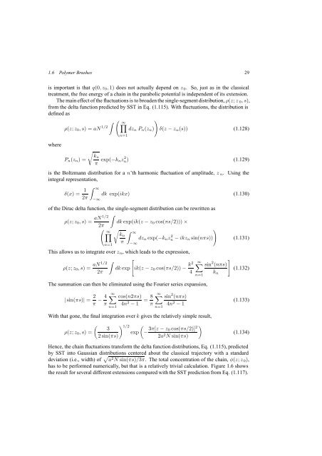
The main effect of the fluctuations is to broaden the single-segment distribution, ρ(z; z 0 ,s),
from the delta function predicted by SST in Eq. (1.115). With fluctuations, the distribution is
defined as
∫ ( )
∏
∞
ρ(z; z 0 ,s)=aN 1/2 dz n P n (z n ) δ(z − z α (s)) (1.128)
n=1
where
√
kn
P n (z n )=
π exp(−k nzn) 2 (1.129)
is the Boltzmann distribution for a n’th harmonic fluctuation of amplitude, z n . Using the
integral representation,
δ(x) = 1
2π
∫ ∞
−∞
dk exp(ikx) (1.130)
of the Dirac delta function, the single-segment distribution can be rewritten as
1/2
∫
aN
ρ(z; z 0 ,s)= dk exp(ik(z − z 0 cos(πs/2))) ×
2π
(
∏ ∞
√ ∫ )
∞
kn
dz n exp(−k n zn 2 − ikz n sin(nπs)) (1.131)
π
n=1 −∞
This allows us to integrate over z n , which leads to the expression,
1/2
∫ [
]
aN
∞∑
ρ(z; z 0 ,s)= dk exp ik(z − z 0 cos(πs/2)) − k2 sin 2 (nπs)
(1.132)
2π
4 k n
n=1
The summation can then be eliminated using the Fourier series expansion,
| sin(πs)| = 2 π − 4 π
∞∑
n=1
cos(n2πs)
4n 2 − 1
= 8 π
∞∑
n=1
sin 2 (nπs)
4n 2 − 1
(1.133)
With that gone, the final integration over k gives the relatively simple result,
( ) 1/2
3
ρ(z; z 0 ,s)=
exp
(− 3π[z − z 0 cos(πs/2)] 2 )
2sin(πs)
2a 2 N sin(πs)
(1.134)
Hence, the chain fluctuations transform the delta function distributions, Eq. (1.115), predicted
by SST into Gaussian distributions centered about the classical trajectory with a standard
deviation (i.e., width) of √ a 2 N sin(πs)/3π. The total concentration of the chain, φ(z; z 0 ),
has to be performed numerically, but that is a relatively trivial calculation. Figure 1.6 shows
the result for several different extensions compared with the SST prediction from Eq. (1.117).