Self-Consistent Field Theory and Its Applications by M. W. Matsen

1.7 Polymer Blends 43
Note that the value of χ is inversely proportional to the segment density, ρ 0 , and thus is not
an invariant quantity; one must be careful of this fact when referring to literature values of χ.
Equation (1.192) is the simplest and by far most common expression for the interactions, but
SCFT is perfectly capable of accommodating more elaborate treatments (Matsen 2002a), if so
desired.
1.7.1 SCFT for a Polymer Blend
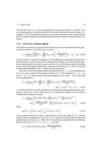
The partition function for a polymer blend is hardly any more involved than that for the polymer
brush in Section 1.6.4. In this case, it becomes
∫ nA
(
1 ∏ ∏n B
Z ∝
˜Dr A,α
˜Dr B,β exp − U[ ˆφ A , ˆφ
)
B ]
δ[1 −
n A !n B !
k B T
ˆφ A − ˆφ B ] (1.194)
α=1
β=1
As before, there is a functional integration over the configuration of each polymer and a Dirac
delta functional is used to enforce the incompressibility condition. Of course, the delta functions
constraining the chain ends are gone, and there is now a Boltzmann weight accounting
for the energy of the segment interactions. Also present are factors of n A ! and n B ! to account
for the indistinguishability of the A- and B-polymers, respectively.
This time, we start by inserting a functional integral over δ[Φ A − ˆφ A ], allowing the operator,
ˆφ A (r), to be swapped with the ordinary function, Φ A (r). This transforms δ[1 − ˆφ A − ˆφ B ]
into δ[1 − Φ A − ˆφ B ], which, in turn, allows the exchange of ˆφ B (r) with 1 − Φ A (r). The result
of this manipulation is
Z ∝
1
n A !n B !
∫
DΦ A
n A
∏
α=1
˜Dr A,α
n B
∏
β=1
(
˜Dr B,β exp − U[Φ )
A, 1 − Φ A ]
×
k B T
δ[Φ A − ˆφ A ]δ[1 − Φ A − ˆφ B ] (1.195)
As with the brush, the two delta functionals are replaced with integral representations analogous
to that in Eq. (1.142), which allows us to complete the integrals over the polymer
configurations, leading to the result,
∫
1
( ρ0
)
Z ∝ DΦ A DW A DW B
n A !n B !
N Q nA
( ρ0
)
A[W A ]
N Q nB
B[W B ] ×
(
exp − U[Φ A, 1 − Φ A ]
+ ρ ∫
)
0
dr[W A Φ A + W B (1 − Φ A )] (1.196)
k B T N
where
∫
( ∫ 1
)
Q γ [W γ ] ∝ ˜Dr γ,α exp − ds W γ (r γ,α (s))
(1.197)
0
is the partition function of a single γ-type polymer in the external field, W γ (r). (For the
purpose of future simplification, a factor of (ρ 0 /N ) n has been extracted from the unspecified
proportionality constant in Eq. (1.196).) Next, the factorials are replaced by the usual Stirling
approximations (e.g., ln(n γ !) ≈ n γ ln(n γ ) − n γ ), giving
∫
(
Z ∝ DΦ A DW A DW B exp − F [Φ )
A,W A ,W B ]
(1.198)
k B T