Self-Consistent Field Theory and Its Applications by M. W. Matsen

1.8 Block Copolymer Melts 61
1.2
f = 0.5
S(k)/N
0.8
0.4
χN=10
9
8
0.0
0 2 4 6 8 10
kaN 1/2
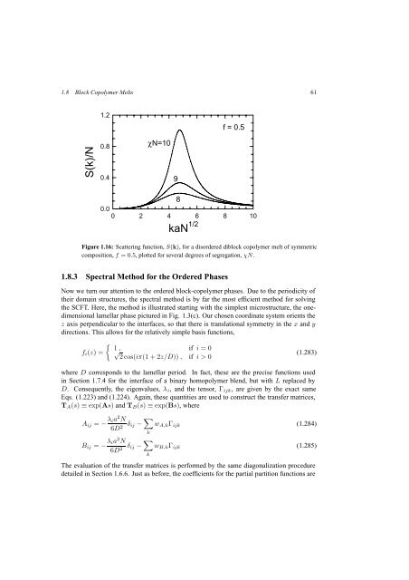
Figure 1.16: Scattering function, S(k), for a disordered diblock copolymer melt of symmetric
composition, f =0.5, plotted for several degrees of segregation, χN.
1.8.3 Spectral Method for the Ordered Phases
Now we turn our attention to the ordered block-copolymer phases. Due to the periodicity of
their domain structures, the spectral method is by far the most efficient method for solving
the SCFT. Here, the method is illustrated starting with the simplest microstructure, the onedimensional
lamellar phase pictured in Fig. 1.3(c). Our chosen coordinate system orients the
z axis perpendicular to the interfaces, so that there is translational symmetry in the x and y
directions. This allows for the relatively simple basis functions,
f i (z) =
{ 1 , if i =0
√
2cos(iπ(1 + 2z/D)) , if i>0
(1.283)
where D corresponds to the lamellar period. In fact, these are the precise functions used
in Section 1.7.4 for the interface of a binary homopolymer blend, but with L replaced by
D. Consequently, the eigenvalues, λ i , and the tensor, Γ ijk , are given by the exact same
Eqs. (1.223) and (1.224). Again, these quantities are used to construct the transfer matrices,
T A (s) ≡ exp(As) and T B (s) ≡ exp(Bs), where
A ij = − λ ia 2 N
6D 2 δ ij − ∑ k
B ij = − λ ia 2 N
6D 2 δ ij − ∑ k
w A,k Γ ijk (1.284)
w B,k Γ ijk (1.285)
The evaluation of the transfer matrices is performed by the same diagonalization procedure
detailed in Section 1.6.6. Just as before, the coefficients for the partial partition functions are