Self-Consistent Field Theory and Its Applications by M. W. Matsen
Self-Consistent Field Theory and Its Applications by M. W. Matsen
Self-Consistent Field Theory and Its Applications by M. W. Matsen

Create successful ePaper yourself
Turn your PDF publications into a flip-book with our unique Google optimized e-Paper software.
8 1 <strong>Self</strong>-consistent field theory <strong>and</strong> its applications<br />
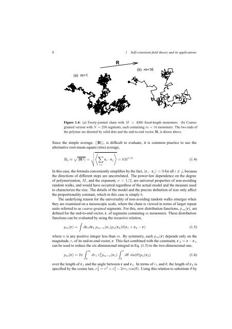
(a) m=1<br />
R<br />
(b) m=16<br />
Figure 1.4: (a) Freely-jointed chain with M = 4000 fixed-length monomers. (b) Coarsegrained<br />
version with N = 250 segments, each containing m =16monomers. The two ends of<br />
the polymer are denoted <strong>by</strong> solid dots <strong>and</strong> the end-to-end vector, R, is drawn above.<br />
Since the simple average, 〈|R|〉, is difficult to evaluate, it is common practice to use the<br />
alternative root-mean-square (rms) average,<br />
R 0 ≡ √ 〈 〉 ∑<br />
〈R 2 〉 = √ r i · r j = bM 1/2 (1.4)<br />
i,j<br />
In this case, the formula conveniently simplifies <strong>by</strong> the fact, 〈r i · r j 〉 =0for all i ≠ j, because<br />
the directions of different steps are uncorrelated. The power-law dependence on the degree<br />
of polymerization, M, <strong>and</strong> the exponent, ν =1/2, are universal properties of non-avoiding<br />
r<strong>and</strong>om walks, <strong>and</strong> would have occurred regardless of the actual model <strong>and</strong> the measure used<br />
to characterize the size. The details of the model <strong>and</strong> the precise definition of size only affect<br />
the proportionality constant, which in this case is simply b.<br />
The underlying reason for the universality of non-avoiding r<strong>and</strong>om walks emerges when<br />
they are examined on a mesoscopic scale, where the chain is viewed in terms of larger repeat<br />
units referred to as coarse-grained segments. For this, new distribution functions, p m (r), are<br />
defined for the end-to-end vector, r, of segments containing m monomers. These distribution<br />
functions can be evaluated <strong>by</strong> using the recursive relation,<br />
∫<br />
p m (r) = dr 1 dr 2 p m−n (r 1 )p n (r 2 )δ(r 1 + r 2 − r) (1.5)<br />
where n is any positive integer less than m. By symmetry, each p m (r) depends only on the<br />
magnitude, r, of its end-to-end vector, r. This fact combined with the constraint, r 2 = r − r 1 ,<br />
can be used to reduce the six-dimensional integral in Eq. (1.5) to the two-dimensional one,<br />
p m (r) =2π<br />
∫ ∞<br />
0<br />
dr 1 r 2 1 p m−n(r 1 )<br />
∫ π<br />
0<br />
dθ sin(θ)p n (r 2 ) (1.6)<br />
over the length of r 1 <strong>and</strong> the angle between r <strong>and</strong> r 1 . In terms of r 1 <strong>and</strong> θ, the length of r 2 is<br />
specified <strong>by</strong> the cosine law, r 2 2 = r2 + r 2 1 − 2rr 1 cos(θ). Using this relation to substitute θ <strong>by</strong>