Self-Consistent Field Theory and Its Applications by M. W. Matsen

More documents

Recommendations

Info

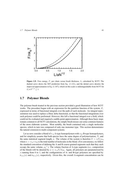
1.7 Polymer Blends 41 4 3 F/nk B T 2 1 0 0.0 0.5 1.0 1.5 2.0 L/aN 1/2 Figure 1.9: Free energy, F , per chain versus brush thickness, L, calculated by SCFT. The dashed curve shows the SST prediction from Eq. (1.121), and the dotted curve denotes the improved approximation in Eq. (1.187), which on this scale is indistinguishable from SCFT for L/aN 1/2 1. 1.7 Polymer Blends The polymer brush treated in the previous section provided a good illustration of how SCFT works. The procedure began with an expression for the partition function of the system, Z, expressed in terms of functional integrals over the path of each molecule. An integral representation was used to replace a Dirac delta functional, so that the functional integrations over each polymer could be performed. However, this left a functional integral over a field, which could not be evaluated and required a saddle-point approximation. Although these basic steps remain common to all SCFT calculations, the simple brush misses out some common features of the more elaborate systems. Most notably, the brush contained only a single molecular species, which in turn was composed of only one monomer type. This section demonstrates the natural extension to multi-component systems. Let us now consider a blend of n A A-type homopolymers with n B B-type homopolymers, and for simplicity assume that both species have the same degree of polymerization, N, and the same statistical segment length, a. The volume of the system is therefore V = nN/ρ 0 , where n = n A +n B is the total number of molecules in the blend. (For convenience, we follow the standard convention of defining the A and B coarse-grained segments such that they each occupy the same volume, ρ −1 0 .) The volume fraction of A-type segments (i.e., composition of the blend) will be denoted by φ ≡ n A N/Vρ 0 . Again, all polymers are parameterized by s running from 0 to 1, and the configurations of A- and B-type polymers are specified by r A,α (s) and r B,α (s), respectively. Given this, the overall A-segment concentration can be
42 1 Self-consistent field theory and its applications expressed as ˆφ A (r) = N ρ 0 ∑n A ∫ 1 α=1 0 ds δ(r − r A,α (s)) (1.188) with an analogous expression specifying the B-segment concentration, ˆφB (r). With the inclusion of two chemically distinct segments, it is no longer possible to sidestep the issue of monomer-monomer interactions. For discussion purposes, assume that the interaction between two monomers, i and j, obeys a simple Lennard-Jones potential, [ ( ) 12 ( ) ] 6 σ σ u(r ij )=ɛ − 2 (1.189) r ij r ij where r ij is their separation. The incompressibility assumption ˆφ A (r)+ˆφ B (r) =1 (1.190) acts to maintain the spacing between neighboring monomers at the minimum of the potential energy, r ij = σ. The detailed shape of the potential is therefore no longer needed; we can simply assume that the interaction energy is −ɛ between neighboring monomers and zero otherwise. In the brush system, all the interactions were the same and thus they added up to a constant energy that could be ignored, assuming the total number of monomer contacts remained more or less fixed. In the blend, however, we must account for the fact that the depth of the potential will differ between the A-A, A-B, and B-B contacts. Noting that the range of the monomer-monomer interactions, σ, is negligible on the coarse-grained scale, the interactions can be treated as contact energies and thus the internal energy can be expressed as U ≡− N 2 ɛ AA ∑ ∫ 2ρ 2 ds dt δ(r A,α (s) − r A,β (t)) − 0 α,β N 2 ɛ AB ∑ ∫ ρ 2 ds dt δ(r A,α (s) − r B,β (t)) − 0 α,β N 2 ɛ BB ∑ ∫ 2ρ 2 ds dt δ(r B,α (s) − r B,β (t)) (1.191) 0 α,β Using the incompressibility assumption, ˆφ A (r)+ ˆφ B (r) =1, this simplifies to U[ ˆφ A , ˆφ B ] k B T = χρ 0 ∫ dr ˆφ A (r) ˆφ B (r) (1.192) where the interaction strengths are grouped together into a single dimensionless parameter, χ ≡ ɛ AA − 2ɛ AB + ɛ BB 2k B Tρ 0 (1.193)
Page 1 and 2: Self-Consistent Field Theory and It
Page 3 and 4: 2 Contents Index 83
Page 5 and 6: 4 1 Self-consistent field theory an
Page 11 and 12: 10 1 Self-consistent field theory a
Page 41: 40 1 Self-consistent field theory a
Page 80 and 81: Bibliography Almdal, K., Rosedale,
Page 82 and 83: BIBLIOGRAPHY 81 Matsen, M. W. and G
Page 84 and 85: Index action 17 binodal point 46 bl

Self-Consistent Field Theory and Its Applications by M. W. Matsen

Create successful ePaper yourself

Delete template?

Save as template?