Self-Consistent Field Theory and Its Applications by M. W. Matsen

60 1 Self-consistent field theory and its applications
w A (r) and w B (r) are sufficiently small such that q(r,f) is well described by Eq. (1.99) with
the field w A (r) and similarly such that q † (r,f) is given by Eq. (1.100) with the field w B (r).
These approximations are then inserted into Eq. (1.274) to give
Q[w A ,w B ]
V
∫
1
≈ 1+
2(2π) 3 dk[S 11 w A (−k)w A (k)+
V
S 22 w B (−k)w B (k)+2S 12 w A (−k)w B (k)] (1.276)
where S 11 ≡ g(x, f), S 22 ≡ g(x, 1 − f), and S 12 ≡ h(x, f)h(x, 1 − f). Differentiating
Q[w A ,w B ] with respect to the Fourier transforms of the fields, as we did in Section 1.7.3,
gives the Fourier transforms of the concentrations,
φ A (k) = −S 11 w A (k) − S 12 w B (k) (1.277)
φ B (k) = −S 22 w B (k) − S 12 w A (k) (1.278)
for all k ≠0. These equations are then inverted to obtain the expressions,
w A (k) = −S 22φ A (k)+S 12 φ B (k)
det(S)
(1.279)
w B (k) = S 12φ A (k) − S 11 φ B (k)
det(S)
(1.280)
for the fields, where det(S) ≡ S 11 S 22 − S12 2 . At this point, the incompressibility condition
can be used to set φ B (k) =−φ A (k), for all k ≠0. Substituting the expressions for the two
fields into that for Q[w A ,w B ], and then inserting that into the logarithm of Eq. (1.273) gives
F
nk B T
= χNf(1 − f)+
N
to second order in |φ A (k)|, where
S −1 (k) =
2(2π) 3 V
∫
k≠0
dk S −1 (k)φ A (−k)φ A (k) (1.281)
g(x, 1)
− 2χ (1.282)
Ndet(S)
is the inverse of the scattering function for a disordered melt. In a somewhat analogous but
considerably more complicated procedure, the scattering functions can also be evaluated for
periodically ordered phases (Yeung et al. 1996; Shi et al. 1996). It involves a very elegant
method akin to band-structure calculations in solid-state physics, providing yet another
example of where SCFT draws upon existing techniques from quantum mechanics.
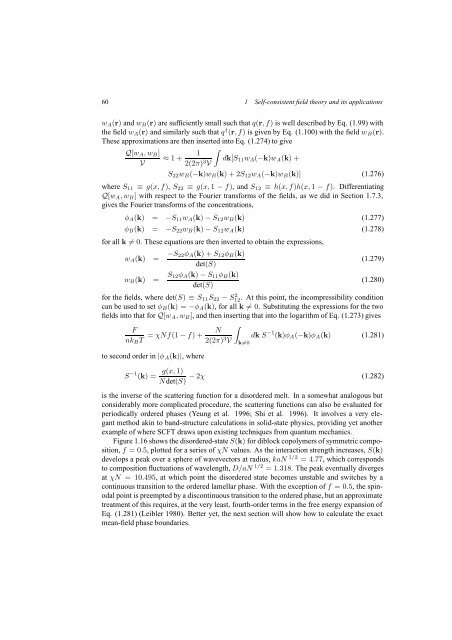
Figure 1.16 shows the disordered-state S(k) for diblock copolymers of symmetric composition,
f =0.5, plotted for a series of χN values. As the interaction strength increases, S(k)
develops a peak over a sphere of wavevectors at radius, kaN 1/2 =4.77, which corresponds
to composition fluctuations of wavelength, D/aN 1/2 =1.318. The peak eventually diverges
at χN =10.495, at which point the disordered state becomes unstable and switches by a
continuous transition to the ordered lamellar phase. With the exception of f =0.5, the spinodal
point is preempted by a discontinuous transition to the ordered phase, but an approximate
treatment of this requires, at the very least, fourth-order terms in the free energy expansion of
Eq. (1.281) (Leibler 1980). Better yet, the next section will show how to calculate the exact
mean-field phase boundaries.