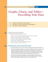
Chapter 2: Graphs, Charts, and Tables--Describing Your Data

More documents

Recommendations

Info

42 CHAPTER 2 • GRAPHS, CHARTS, AND TABLES—DESCRIBING YOUR DATA SUMMARY Developing Frequency Distributions for Continuous Variables To develop a continuous data frequency distribution, perform the following steps: 1. Determine the desired number of classes or groups. The rule of thumb is to use 5 to 20 classes. The 2 k n rule can be used. 2. Determine the minimum class width using: Largest Value Smallest Value W Number of Classes Round the class width up to a more convenient value. 3. Define the class boundaries, making sure that the classes that are formed are mutually exclusive and all-inclusive. Ideally, the classes should have equal widths and should all contain at least one observation. 4. Count the number of values in each class. EXAMPLE 2-3 Frequency Distribution for Continuous Variables TRY PROBLEM 2.9 Airport Security Screening Example 2-1 referred to the international travel difficulties after the September 11, 2001, attack on the World Trade Center in New York City and the Pentagon in Washington D.C. As a result, airports throughout the world have stepped up their security, and passengers have had to spend more time waiting to pass through security screening. At the Miami, Florida, airport, officials each week select a random sample of passengers. For each person selected, the time spent in the security screening line is recorded. The waiting times (already sorted from high to low), in seconds, for one such sample of 72 passengers are as follows: 35 339 650 864 1,025 1,261 38 340 655 883 1,028 1,280 48 395 669 883 1,036 1,290 53 457 703 890 1,044 1,312 70 478 730 934 1,087 1,341 99 501 763 951 1,091 1,355 138 521 788 969 1,126 1,357 164 556 789 985 1,176 1,360 220 583 789 993 1,199 1,414 265 595 802 997 1,199 1,436 272 596 822 999 1,237 1,479 312 604 851 1,018 1,242 1,492 The airport security manger wishes to construct a frequency distribution for the time passengers wait for security screening. The frequency distribution is determined as follows: Step 1 Group the data into classes. The number of classes is arbitrary but typically will be between 5 and 20, depending on the volume of data. In this example, we have n 72 data items. Using the 2 k n guideline we get k 7 classes (2 7 126 72). Step 2 Determine the class width. Largest Value Smallest Value W Number of Classes 1, 492 35 208. 1429 225 7 Note, we have rounded the class width up from the minimum required value of 208.1429 to the more convenient value of 225.
CHAPTER 2 • GRAPHS, CHARTS, AND TABLES—DESCRIBING YOUR DATA 43 Step 3 Define the class boundaries. 0 and under 225 225 and under 450 450 and under 675 675 and under 900 900 and under 1,125 1,125 and under 1,350 1,350 and under 1,575 These classes are mutually exclusive, all-inclusive, and have equal widths. Step 4 Count the number of values in each class. Waiting Time Frequency 0 and under 225 9 225 and under 450 6 450 and under 675 12 675 and under 900 13 900 and under 1,125 14 1,125 and under 1,350 11 1,350 and under 1,575 7 This frequency distribution shows that for this sample of passengers, most people wait between 450 and 1,350 seconds. Frequency Histogram A graph of a frequency distribution with the horizontal axis showing the classes, the vertical axis showing the frequency count, and (for equal class widths) the rectangles having a height equal to the frequency in each class. CHAPTER OUTCOME #2 Business Application Excel and Minitab Tutorial Histograms Although frequency distributions are useful for analyzing large sets of data, they are presented in table format and may not be as visually informative as a graph. If a frequency distribution has been developed from a quantitative variable, a frequency histogram can be constructed directly from the frequency distribution. In many cases, the histogram offers a superior format for transforming the data into useful information. (Note, histograms cannot be constructed from a frequency distribution where the variable of interest is qualitative. However, a similar graph, called a bar chart, is used when qualitative data are involved.) A histogram shows three general types of information: 1. It provides a visual indication of where the approximate center of the data is. Look for the center point along the horizontal axes in the histograms in Figure 2.3. Even though the shapes of the histograms are the same, there is a clear difference in where the data are centered. 2. We can gain an understanding of the degree of spread (or variation) in the data. The more the data cluster around the center, the smaller the variation in the data. If the data are spread out from the center, the data exhibit greater variation. The examples in Figure 2.4 all have the same center but are different in terms of spread. 3. We can observe the shape of the distribution. Is it reasonably flat, is it weighted to one side or the other, is it balanced around the center, or is it bell-shaped? CAPITAL CREDIT UNION Even for applications with small amounts of data, such as the Blockbuster example, constructing grouped data frequency distributions and histograms is a time-consuming process. Decision makers may hesitate to try different numbers of classes and different class limits because of the effort involved and the “best” presentation of the data may be missed.
Page 1 and 2: Chapter TWO Graphs, Charts, and Tab
Page 3 and 4: CHAPTER 2 • GRAPHS, CHARTS, AND T
Page 11: CHAPTER 2 • GRAPHS, CHARTS, AND T

Chapter 2: Graphs, Charts, and Tables--Describing Your Data

You also want an ePaper? Increase the reach of your titles

Delete template?

Save as template?