Numerical Simulation of the Dynamics of Turbulent Swirling Flames

5.7 Flame Transfer Function Model
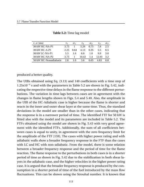
Table 5.2: Time lag model
τ, σ [ms] τ 1 σ 1 τ 2 σ 2 τ 3 σ 3
30 kW HC-NA-P1 3.75 1 5.29 0.75 7.8 2.5
30 kW HC-A-P1 2.25 0.64 4.13 0.35 5.5 0.5
30 kW LC-NA-P1 5.3 1.6 6.0 1.0 9.9 3.0
30 kW HC-NA-P2 3.75 1 10.42 1.4 12.93 3.2
50 kW HC-Nonadiabatic 2.8 1.0 3.6 0.65 4.83 0.8
produced a better quality.
The UIRs obtained using Eq. (3.13) and 140 coefficients with a time step of
1.25x10 −4 s and with the parameters in Table 5.2 are shown in Fig. 5.42, indicating
the respective time delays in the flame response to the different perturbations.
The variation in time lags between cases are in agreement with the
changes in flame lengths shown in Figs. 5.4 and 5.40. Also, the amplitude in
the UIR of the HC-Adiabatic case is higher because the flame is shorter and
reacts in the inner and outer shear layer at the same time. Thus, the standard
deviations in the model are smaller than in the other cases, indicating that
the response is in a narrower period of time. The identified FTF for 50 kW is
fitted also with the model and its parameters are included in Table 5.2. The
FTFs obtained using the model are shown in Fig. 5.43 with very good agreement
with the identified FTFs. Additionally, the sum of all coefficients between
cases is equal to unity, in agreement with the zero frequency limit for
the amplitude of the FTF [159]. The cases with higher power rating and with
adiabatic walls show a broader frequency response in the FTF than the cases
with LC and HC with non-adiabatic. From the model, there is some relation
between a broader frequency response and the period of time for the flame
reaction. The flame response to the perturbations in both cases is in a shorter
period of time as shown in Fig. 5.42 due to the stabilization in both shear layers
in the adiabatic case, and the higher velocities in the higher power rating
case. It is argued that the broader frequency response is produced by the consumption
in a shorter period of time of the fuel introduced by the mass flow
fluctuations. This can be shown using the Strouhal number. It is known that
113