Numerical Simulation of the Dynamics of Turbulent Swirling Flames

Stability Analysis with Low-Order Network Models
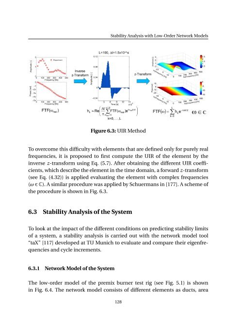
Figure 6.3: UIR Method
To overcome this difficulty with elements that are defined only for purely real
frequencies, it is proposed to first compute the UIR of the element by the
inverse z-transform using Eq. (5.7). After obtaining the different UIR coefficients,
which describe the element in the time domain, a forward z-transform
(see Eq. (4.32)) is applied evaluating the element with complex frequencies
(ω ∈ C). A similar procedure was applied by Schuermans in [177]. A scheme of
the procedure is shown in Fig. 6.3.
6.3 Stability Analysis of the System
To look at the impact of the different conditions on predicting stability limits
of a system, a stability analysis is carried out with the network model tool
“taX” [117] developed at TU Munich to evaluate and compare their eigenfrequencies
and cycle increments.
6.3.1 Network Model of the System
The low-order model of the premix burner test rig (see Fig. 5.1) is shown
in Fig. 6.4. The network model consists of different elements as ducts, area
128