Numerical Simulation of the Dynamics of Turbulent Swirling Flames

6.2 Low-order Network Models
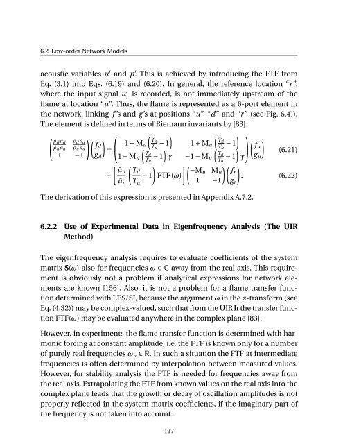
acoustic variables u ′ and p ′ . This is achieved by introducing the FTF from
Eq. (3.1) into Eqs. (6.19) and (6.20). In general, the reference location “r ”,
where the input signal u r
′ is recorded, is not immediately upstream of the
flame at location “u”. Thus, the flame is represented as a 6-port element in
the network, linking f ’s and g ’s at positions “u”, “d” and “r ” (see Fig. 6.4)).
The element is defined in terms of Riemann invariants by [83]:
( ρd
) ⎛ ( )
( ) ⎞
a d ρ d a d ( )
ρ u a u ρ u a fd u
= ⎝
1 − M Td
Td
)
u T u
− 1 1 + M u T u
− 1
( )
( ) ⎠(
fu
1 −1 g Td
Td
(6.21)
d 1 − M u T u
− 1 γ −1 − M u T u
− 1 γ g u
( ) ]( )( )
[ūu Td
−Mu M u fr
+ − 1 FTF(ω)
. (6.22)
ū r T u 1 −1 g r
The derivation of this expression is presented in Appendix A.7.2.
6.2.2 Use of Experimental Data in Eigenfrequency Analysis (The UIR
Method)
The eigenfrequency analysis requires to evaluate coefficients of the system
matrix S(ω) also for frequencies ω ∈ C away from the real axis. This requirement
is obviously not a problem if analytical expressions for network elements
are known [156]. Also, it is not a problem for a flame transfer function
determined with LES/SI, because the argument ω in the z-transform (see
Eq. (4.32)) may be complex-valued, such that from the UIR h the transfer function
FTF(ω) may be evaluated anywhere in the complex plane [83].
However, in experiments the flame transfer function is determined with harmonic
forcing at constant amplitude, i.e. the FTF is known only for a number
of purely real frequencies ω n ∈ R. In such a situation the FTF at intermediate
frequencies is often determined by interpolation between measured values.
However, for stability analysis the FTF is needed for frequencies away from
the real axis. Extrapolating the FTF from known values on the real axis into the
complex plane leads that the growth or decay of oscillation amplitudes is not
properly reflected in the system matrix coefficients, if the imaginary part of
the frequency is not taken into account.
127