Numerical Simulation of the Dynamics of Turbulent Swirling Flames

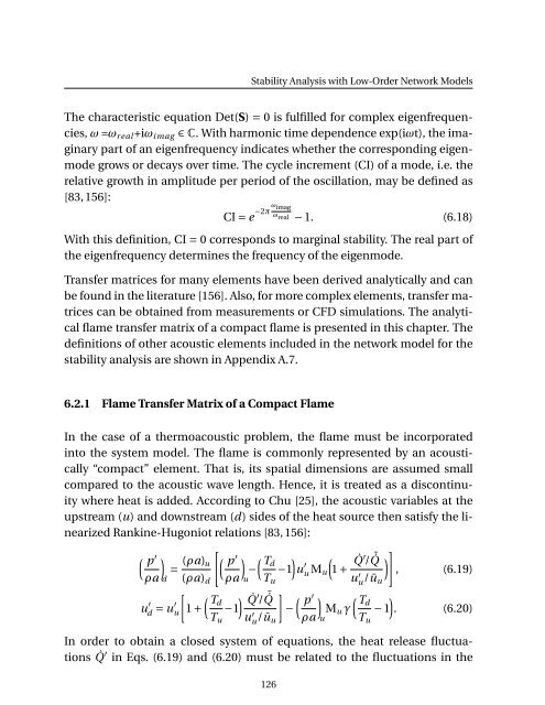
Stability Analysis with Low-Order Network Models
The characteristic equation Det(S) = 0 is fulfilled for complex eigenfrequencies,
ω =ω r eal +iω i mag ∈ C. With harmonic time dependence exp(iωt), the imaginary
part of an eigenfrequency indicates whether the corresponding eigenmode
grows or decays over time. The cycle increment (CI) of a mode, i.e. the
relative growth in amplitude per period of the oscillation, may be defined as
[83, 156]:
CI = e −2π ω imag
ω real − 1. (6.18)
With this definition, CI = 0 corresponds to marginal stability. The real part of
the eigenfrequency determines the frequency of the eigenmode.
Transfer matrices for many elements have been derived analytically and can
be found in the literature [156]. Also, for more complex elements, transfer matrices
can be obtained from measurements or CFD simulations. The analytical
flame transfer matrix of a compact flame is presented in this chapter. The
definitions of other acoustic elements included in the network model for the
stability analysis are shown in Appendix A.7.
6.2.1 Flame Transfer Matrix of a Compact Flame
In the case of a thermoacoustic problem, the flame must be incorporated
into the system model. The flame is commonly represented by an acoustically
“compact” element. That is, its spatial dimensions are assumed small
compared to the acoustic wave length. Hence, it is treated as a discontinuity
where heat is added. According to Chu [25], the acoustic variables at the
upstream (u) and downstream (d) sides of the heat source then satisfy the linearized
Rankine-Hugoniot relations [83, 156]:
[
( p
′ )
= (ρa) (
u p
′ )
ρa d (ρa) d ρa
[
u ′ d = u′ u
1 +
u
( Td
−
( Td
) ˙Q ′ / ¯˙Q −1
T u u u ′ /ū u
)
−1 u ′ u
T M u
u
]
(
1 + ˙Q ′ / ¯˙Q ) ]
u u ′ /ū , (6.19)
u
( p
′ ) ( Td
)
− M u γ − 1 . (6.20)
ρa u T u
In order to obtain a closed system of equations, the heat release fluctuations
˙Q ′ in Eqs. (6.19) and (6.20) must be related to the fluctuations in the
126