Numerical Simulation of the Dynamics of Turbulent Swirling Flames

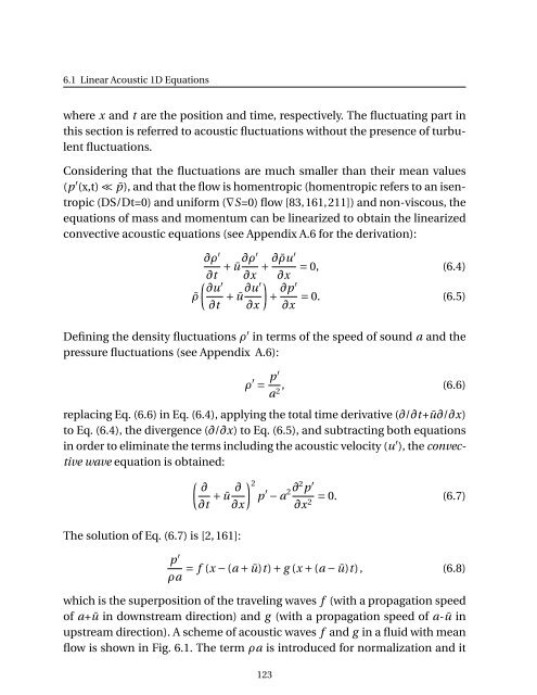
6.1 Linear Acoustic 1D Equations
where x and t are the position and time, respectively. The fluctuating part in
this section is referred to acoustic fluctuations without the presence of turbulent
fluctuations.
Considering that the fluctuations are much smaller than their mean values
(p ′ (x,t) ≪ ¯p), and that the flow is homentropic (homentropic refers to an isentropic
(DS/Dt=0) and uniform (∇S=0) flow [83,161,211]) and non-viscous, the
equations of mass and momentum can be linearized to obtain the linearized
convective acoustic equations (see Appendix A.6 for the derivation):
∂ρ ′
∂t + ū ∂ρ′
∂x + ∂ ¯ρu′ = 0, (6.4)
( ∂x
∂u
′
)
¯ρ
∂t + ū ∂u′ + ∂p′ = 0. (6.5)
∂x ∂x
Defining the density fluctuations ρ ′ in terms of the speed of sound a and the
pressure fluctuations (see Appendix A.6):
ρ ′ = p′
a 2 , (6.6)
replacing Eq. (6.6) in Eq. (6.4), applying the total time derivative (∂/∂t+ū∂/∂x)
to Eq. (6.4), the divergence (∂/∂x) to Eq. (6.5), and subtracting both equations
in order to eliminate the terms including the acoustic velocity (u ′ ), the convective
wave equation is obtained:
( ∂
∂t + ū ∂
∂x
The solution of Eq. (6.7) is [2, 161]:
) 2
p ′ − a 2 ∂2 p ′
= 0. (6.7)
∂x2 p ′
ρa
= f (x − (a + ū)t) + g (x + (a − ū)t), (6.8)
which is the superposition of the traveling waves f (with a propagation speed
of a+ū in downstream direction) and g (with a propagation speed of a-ū in
upstream direction). A scheme of acoustic waves f and g in a fluid with mean
flow is shown in Fig. 6.1. The term ρa is introduced for normalization and it
123