Numerical Simulation of the Dynamics of Turbulent Swirling Flames
Numerical Simulation of the Dynamics of Turbulent Swirling Flames
Numerical Simulation of the Dynamics of Turbulent Swirling Flames

Create successful ePaper yourself
Turn your PDF publications into a flip-book with our unique Google optimized e-Paper software.
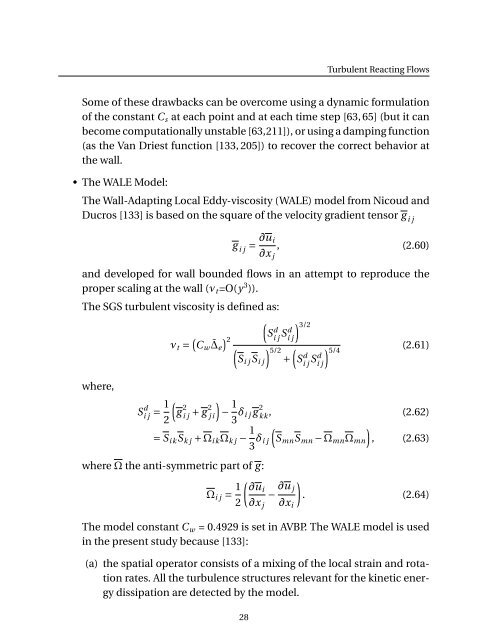
<strong>Turbulent</strong> Reacting Flows<br />
Some <strong>of</strong> <strong>the</strong>se drawbacks can be overcome using a dynamic formulation<br />
<strong>of</strong> <strong>the</strong> constant C s at each point and at each time step [63, 65] (but it can<br />
become computationally unstable [63,211]), or using a damping function<br />
(as <strong>the</strong> Van Driest function [133, 205]) to recover <strong>the</strong> correct behavior at<br />
<strong>the</strong> wall.<br />
• The WALE Model:<br />
The Wall-Adapting Local Eddy-viscosity (WALE) model from Nicoud and<br />
Ducros [133] is based on <strong>the</strong> square <strong>of</strong> <strong>the</strong> velocity gradient tensor g i j<br />
g i j<br />
= ∂u i<br />
∂x j<br />
, (2.60)<br />
and developed for wall bounded flows in an attempt to reproduce <strong>the</strong><br />
proper scaling at <strong>the</strong> wall (ν t =O(y 3 )).<br />
The SGS turbulent viscosity is defined as:<br />
ν t = ( C w ¯∆ e<br />
) 2<br />
(<br />
S d i j Sd i j<br />
) 3/2<br />
) 5/2 ( ) 5/4<br />
(2.61)<br />
(S i j S i j + S d i j Sd i j<br />
where,<br />
S d i j = 1 ( )<br />
g 2 i j<br />
2<br />
+ g 2 j i<br />
− 1 3 δ i j g 2 kk , (2.62)<br />
= S i k S k j + Ω i k Ω k j − 1 )<br />
3 δ i j<br />
(S mn S mn − Ω mn Ω mn , (2.63)<br />
where Ω <strong>the</strong> anti-symmetric part <strong>of</strong> g :<br />
Ω i j = 1 ( ∂ui<br />
− ∂u )<br />
j<br />
. (2.64)<br />
2 ∂x j ∂x i<br />
The model constant C w = 0.4929 is set in AVBP. The WALE model is used<br />
in <strong>the</strong> present study because [133]:<br />
(a) <strong>the</strong> spatial operator consists <strong>of</strong> a mixing <strong>of</strong> <strong>the</strong> local strain and rotation<br />
rates. All <strong>the</strong> turbulence structures relevant for <strong>the</strong> kinetic energy<br />
dissipation are detected by <strong>the</strong> model.<br />
28