Comprehensive Risk Assessment for Natural Hazards - Planat
Comprehensive Risk Assessment for Natural Hazards - Planat
Comprehensive Risk Assessment for Natural Hazards - Planat

Create successful ePaper yourself
Turn your PDF publications into a flip-book with our unique Google optimized e-Paper software.
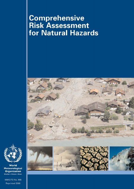
<strong>Comprehensive</strong><br />
<strong>Risk</strong> <strong>Assessment</strong><br />
<strong>for</strong> <strong>Natural</strong> <strong>Hazards</strong><br />
WMO/TD No. 955<br />
Reprinted 2006
Cover photos: Schweizer Luftwaffe, Randy H. Williams, DigitalGlobe<br />
© 1999, World Meteorological Organization<br />
WMO/TD No. 955<br />
Reprinted 2006<br />
NOTE<br />
The designations employed and the presentation of material in this<br />
publication do not imply the expression of any opinion whatsoever on the<br />
part of any of the participating agencies concerning the legal status of any<br />
country, territory, city or area, or of its authorities, or concerning the<br />
delimitation of its frontiers or boundaries.
CONTENTS<br />
AUTHORS AND EDITORS . . . . . . . . . . . . . . . . . . . . .<br />
FOREWORD . . . . . . . . . . . . . . . . . . . . . . . . . . . . . . . . . .<br />
Page<br />
v<br />
vii<br />
Page<br />
2.7 Conclusion . . . . . . . . . . . . . . . . . . . . . . . . . . . . . . . . 16<br />
2.8 Glossary of terms . . . . . . . . . . . . . . . . . . . . . . . . . . 16<br />
2.9 References . . . . . . . . . . . . . . . . . . . . . . . . . . . . . . . . . 16<br />
CHAPTER 1 — INTRODUCTION . . . . . . . . . . . . . . . 1<br />
1.1 Project history . . . . . . . . . . . . . . . . . . . . . . . . . . . . . 1<br />
1.2 Framework <strong>for</strong> risk assessment . . . . . . . . . . . . . . . 2<br />
1.2.1 Definition of terms . . . . . . . . . . . . . . . . . . . 2<br />
1.2.2 Philosophy of risk assessment . . . . . . . . . . 2<br />
1.2.3 <strong>Risk</strong> aversion . . . . . . . . . . . . . . . . . . . . . . . . 4<br />
1.3 The future . . . . . . . . . . . . . . . . . . . . . . . . . . . . . . . . . 4<br />
1.4 References . . . . . . . . . . . . . . . . . . . . . . . . . . . . . . . . . 5<br />
CHAPTER 2 — METEOROLOGICAL HAZARDS . . 6<br />
2.1 Introduction . . . . . . . . . . . . . . . . . . . . . . . . . . . . . . . 6<br />
2.2 Description of the event . . . . . . . . . . . . . . . . . . . . . 6<br />
2.2.1 Tropical storm . . . . . . . . . . . . . . . . . . . . . . . 6<br />
2.2.2 Necessary conditions <strong>for</strong> tropical storm<br />
genesis . . . . . . . . . . . . . . . . . . . . . . . . . . . . . 6<br />
2.3 Meteorological hazards assessment . . . . . . . . . . . 7<br />
2.3.1 Physical characteristics . . . . . . . . . . . . . . . . 7<br />
2.3.1.1 Tropical storms . . . . . . . . . . . . . . . 8<br />
2.3.1.2 Extratropical storms . . . . . . . . . . . 8<br />
2.3.2 Wind . . . . . . . . . . . . . . . . . . . . . . . . . . . . . 8<br />
2.3.3 Rain loads . . . . . . . . . . . . . . . . . . . . . . . . . . . 8<br />
2.3.4 Rainfall measurements . . . . . . . . . . . . . . . . 9<br />
2.3.5 Storm surge . . . . . . . . . . . . . . . . . . . . . . . . . 9<br />
2.3.6 Windwave . . . . . . . . . . . . . . . . . . . . . . . . . . . 9<br />
2.3.7 Extreme precipitation . . . . . . . . . . . . . . . . . 10<br />
2.3.7.1 Rain . . . . . . . . . . . . . . . . . . . . . . . . . 10<br />
2.3.7.2 Snow and hail . . . . . . . . . . . . . . . . . 10<br />
2.3.7.3 Ice loads . . . . . . . . . . . . . . . . . . . . . 10<br />
2.3.8 Drought . . . . . . . . . . . . . . . . . . . . . . . . . . . . . 10<br />
2.3.9 Tornadoes . . . . . . . . . . . . . . . . . . . . . . . . . . . 10<br />
2.3.10 Heatwaves . . . . . . . . . . . . . . . . . . . . . . . . . . . 11<br />
2.4 Techniques <strong>for</strong> hazard analysis and<br />
<strong>for</strong>ecasting . . . . . . . . . . . . . . . . . . . . . . . . . . . . . . . . 11<br />
2.4.1 Operational techniques . . . . . . . . . . . . . . . 11<br />
2.4.2 Statistical methods . . . . . . . . . . . . . . . . . . . 12<br />
2.5 Anthropogenic influence on meteorological<br />
hazards . . . . . . . . . . . . . . . . . . . . . . . . . . . . . . . . . . . 14<br />
2.6 Meteorological phenomena: risk assessment . . . 14<br />
2.6.1 General . . . . . . . . . . . . . . . . . . . . . . . . . . . . . 14<br />
2.6.2 Steps in risk assessment . . . . . . . . . . . . . . . 15<br />
2.6.3 Phases of hazard warning . . . . . . . . . . . . . 15<br />
2.6.3.1 General preparedness . . . . . . . . . . 15<br />
2.6.3.2 The approach of the<br />
phenomenon . . . . . . . . . . . . . . . . . 15<br />
2.6.3.3 During the phenomenon . . . . . . . 15<br />
2.6.3.4 The aftermath . . . . . . . . . . . . . . . . 16<br />
CHAPTER 3 — HYDROLOGICAL HAZARDS . . . . 18<br />
3.1 Introduction . . . . . . . . . . . . . . . . . . . . . . . . . . . . . 18<br />
3.2 Description of the hazard . . . . . . . . . . . . . . . . . . . 18<br />
3.3 Causes of flooding and flood hazards . . . . . . . . . 19<br />
3.3.1 Introduction . . . . . . . . . . . . . . . . . . . . . . . . . 19<br />
3.3.2 Meteorological causes of river floods and<br />
space-time characteristics . . . . . . . . . . . . . 20<br />
3.3.3 Hydrological contributions to floods . . . . 20<br />
3.3.4 Coastal and lake flooding . . . . . . . . . . . . . 21<br />
3.3.5 Anthropogenic factors, stationarity, and<br />
climate change . . . . . . . . . . . . . . . . . . . . . . . 21<br />
3.4 Physical characteristics of floods . . . . . . . . . . . . . 21<br />
3.4.1 Physical hazards . . . . . . . . . . . . . . . . . . . . . . 21<br />
3.4.2 Measurement techniques . . . . . . . . . . . . . . 21<br />
3.5 Techniques <strong>for</strong> flood hazard assessment . . . . . . . 22<br />
3.5.1 Basic principles . . . . . . . . . . . . . . . . . . . . . . 22<br />
3.5.2 Standard techniques <strong>for</strong> watersheds with<br />
abundant data . . . . . . . . . . . . . . . . . . . . . . . 23<br />
3.5.3 Refinements to the standard<br />
techniques . . . . . . . . . . . . . . . . . . . . . . . . . . . 24<br />
3.5.3.1 Regionalization . . . . . . . . . . . . . . . 24<br />
3.5.3.2 Paleoflood and historical data . . . 25<br />
3.5.4 Alternative data sources and methods . . . 25<br />
3.5.4.1 Extent of past flooding . . . . . . . . . 25<br />
3.5.4.2 Probable maximum flood and<br />
rainfall-runoff modelling . . . . . . . 25<br />
3.5.5 Methods <strong>for</strong> watersheds with limited<br />
streamflow data . . . . . . . . . . . . . . . . . . . . . . 26<br />
3.5.6 Methods <strong>for</strong> watersheds with limited<br />
topographic data . . . . . . . . . . . . . . . . . . . . . 26<br />
3.5.7 Methods <strong>for</strong> watersheds with no data . . . 26<br />
3.5.7.1 Estimation of flood discharge . . . 26<br />
3.5.7.2 Recognition of areas subject to<br />
inundation . . . . . . . . . . . . . . . . . . . 26<br />
3.5.8 Lakes and reservoirs . . . . . . . . . . . . . . . . . . 26<br />
3.5.9 Storm surge and tsumani . . . . . . . . . . . . . . 26<br />
3.6 Flood risk assessment . . . . . . . . . . . . . . . . . . . . . . . 27<br />
3.7 Data requirements and sources . . . . . . . . . . . . . . . 27<br />
3.8 Anthropogenic factors and climate change . . . . 28<br />
3.8.1 Anthropogenic contributions to<br />
flooding . . . . . . . . . . . . . . . . . . . . . . . . . . . . . 28<br />
3.8.2 Climate change and variability . . . . . . . . . 28<br />
3.9 Practical aspects of applying the<br />
techniques . . . . . . . . . . . . . . . . . . . . . . . . . . . . . . . . 29<br />
3.10 Presentation of hazard assessments . . . . . . . . . . . 29<br />
3.11 Related preparedness schemes . . . . . . . . . . . . . . . 30<br />
3.12 Glossary of terms . . . . . . . . . . . . . . . . . . . . . . . . . . 30<br />
3.13 References . . . . . . . . . . . . . . . . . . . . . . . . . . . . . . . . . 31
iv<br />
Contents<br />
Page<br />
CHAPTER 4 — VOLCANIC HAZARDS . . . . . . . . . . 34<br />
4.1 Introduction to volcanic risks . . . . . . . . . . . . . . . . 34<br />
4.2 Description and characteristics of the main<br />
volcanic hazards . . . . . . . . . . . . . . . . . . . . . . . . . . . 36<br />
4.2.1 Direct hazards . . . . . . . . . . . . . . . . . . . . . . . 36<br />
4.2.2 Indirect hazards . . . . . . . . . . . . . . . . . . . . . . 37<br />
4.3 Techniques <strong>for</strong> volcanic hazard assessment . . . . 37<br />
4.3.1 Medium- and long-term hazard<br />
assessment: zoning . . . . . . . . . . . . . . . . . . . 37<br />
4.3.2 Short-term hazard assessment:<br />
monitoring . . . . . . . . . . . . . . . . . . . . . . . . . . 38<br />
4.4 Data requirements and sources . . . . . . . . . . . . . . . 39<br />
4.4.1 Data sources . . . . . . . . . . . . . . . . . . . . . . . . . 39<br />
4.4.2 Monitoring — Data management . . . . . . 39<br />
4.5 Practical aspects of applying the techniques . . . 40<br />
4.5.1 Practice of hazard zoning mapping . . . . . 40<br />
4.5.2 Practice of monitoring . . . . . . . . . . . . . . . . 41<br />
4.6 Presentation of hazard and risk<br />
assessment maps . . . . . . . . . . . . . . . . . . . . . . . . . . . 41<br />
4.7 Related mitigation scheme . . . . . . . . . . . . . . . . . . . 41<br />
4.8 Glossary of terms . . . . . . . . . . . . . . . . . . . . . . . . . . 42<br />
4.9 References . . . . . . . . . . . . . . . . . . . . . . . . . . . . . . . . . 44<br />
CHAPTER 5 — SEISMIC HAZARDS . . . . . . . . . . . . . 46<br />
5.1 Introduction . . . . . . . . . . . . . . . . . . . . . . . . . . . . . 46<br />
5.2 Description of earthquake hazards . . . . . . . . . . . 46<br />
5.3 Causes of earthquake hazards . . . . . . . . . . . . . . . . 48<br />
5.3.1 <strong>Natural</strong> seismicity . . . . . . . . . . . . . . . . . . . . 48<br />
5.3.2 Induced seismicity . . . . . . . . . . . . . . . . . . . 48<br />
5.4 Characteristics of earthquake hazards . . . . . . . . . 49<br />
5.4.1 Application . . . . . . . . . . . . . . . . . . . . . . . . . . 49<br />
5.4.2 Ground shaking . . . . . . . . . . . . . . . . . . . . . . 49<br />
5.4.3 Surface faulting . . . . . . . . . . . . . . . . . . . . . . 49<br />
5.4.4 Liquefaction . . . . . . . . . . . . . . . . . . . . . . . . . 49<br />
5.4.5 Landslides . . . . . . . . . . . . . . . . . . . . . . . . . . . 49<br />
5.4.6 Tectonic de<strong>for</strong>mation . . . . . . . . . . . . . . . . . 49<br />
5.5 Techniques <strong>for</strong> earthquake hazard assessment . . 50<br />
5.5.1 Principles . . . . . . . . . . . . . . . . . . . . . . . . . . . 50<br />
5.5.2 Standard techniques . . . . . . . . . . . . . . . . . . 50<br />
5.5.3 Refinements to standard techniques . . . . 51<br />
5.5.4 Alternative techniques . . . . . . . . . . . . . . . . 53<br />
5.6 Data requirements and sources . . . . . . . . . . . . . . . 53<br />
5.6.1 Seismicity data . . . . . . . . . . . . . . . . . . . . . . . 53<br />
5.6.2 Seismotectonic data . . . . . . . . . . . . . . . . . . 53<br />
5.6.3 Strong ground motion data . . . . . . . . . . . . 53<br />
5.6.4 Macroseismic data . . . . . . . . . . . . . . . . . . . . 54<br />
5.6.5 Spectral data . . . . . . . . . . . . . . . . . . . . . . . . . 54<br />
5.6.6 Local amplification data . . . . . . . . . . . . . . . 54<br />
5.7 Anthropogenic factors . . . . . . . . . . . . . . . . . . . . . . 54<br />
5.8 Practical aspects . . . . . . . . . . . . . . . . . . . . . . . . . . . 54<br />
5.9 Presentation of hazard assessments . . . . . . . . . . . 54<br />
5.9.1 Probability terms . . . . . . . . . . . . . . . . . . . . . 54<br />
Page<br />
5.9.2 Hazard maps . . . . . . . . . . . . . . . . . . . . . . . . 54<br />
5.9.3 Seismic zoning . . . . . . . . . . . . . . . . . . . . . . . 55<br />
5.10 Preparedness and mitigation . . . . . . . . . . . . . . . . . 55<br />
5.11 Glossary of terms . . . . . . . . . . . . . . . . . . . . . . . . . . 55<br />
5.12 References . . . . . . . . . . . . . . . . . . . . . . . . . . . . . . . . . 59<br />
CHAPTER 6 — HAZARD ASSESSMENT AND LAND-<br />
USE PLANNING IN SWITZERLAND FOR SNOW<br />
AVALANCHES, FLOODS AND LANDSLIDES . . . . . 61<br />
6.1 Switzerland: A hazard-prone country . . . . . . . . . 61<br />
6.2 Regulations . . . . . . . . . . . . . . . . . . . . . . . . . . . . . . . . 61<br />
6.3 Hazard management . . . . . . . . . . . . . . . . . . . . . . . 62<br />
6.3.1 Hazard identification: What might<br />
happen and where? . . . . . . . . . . . . . . . . . . . 62<br />
6.3.2 The hazard assessment: How and<br />
when can it happen? . . . . . . . . . . . . . . . . . . 62<br />
6.4 Codes of practice <strong>for</strong> land-use planning . . . . . . . 64<br />
6.5 Concluding remarks . . . . . . . . . . . . . . . . . . . . . . . . 64<br />
6.6 References . . . . . . . . . . . . . . . . . . . . . . . . . . . . . . . . . 64<br />
CHAPTER 7— ECONOMIC ASPECTS OF<br />
VULNERABILITY . . . . . . . . . . . . . . . . . . . . . . . . . . . . . 66<br />
7.1 Vulnerability . . . . . . . . . . . . . . . . . . . . . . . . . . . . . 66<br />
7.2 Direct damages . . . . . . . . . . . . . . . . . . . . . . . . . . . . 67<br />
7.2.1 Structures and contents . . . . . . . . . . . . . . . 67<br />
7.2.2 Value of life and cost of injuries . . . . . . . . 68<br />
7.3 Indirect damages . . . . . . . . . . . . . . . . . . . . . . . . . . . 71<br />
7.3.1 General considerations . . . . . . . . . . . . . . . . 71<br />
7.3.2 The input-output (I-O) model . . . . . . . . . 71<br />
7.4 Glossary of terms . . . . . . . . . . . . . . . . . . . . . . . . . . 74<br />
7.5 References . . . . . . . . . . . . . . . . . . . . . . . . . . . . . . . . . 76<br />
CHAPTER 8 — STRATEGIES FOR RISK<br />
ASSESSMENT — CASE STUDIES . . . . . . . . . . . . . . . 77<br />
8.1 Implicit societally acceptable hazards . . . . . . . . . 77<br />
8.2 Design of coastal protection works in The<br />
Netherlands . . . . . . . . . . . . . . . . . . . . . . . . . . . . . . . 78<br />
8.3 Minimum life-cycle cost earthquake design . . . . 79<br />
8.3.1 Damage costs . . . . . . . . . . . . . . . . . . . . . . . . 81<br />
8.3.2 Determination of structural damage<br />
resulting from earthquakes . . . . . . . . . . . . 82<br />
8.3.3 Earthquake occurrence model . . . . . . . . . 82<br />
8.4 Alternative approaches <strong>for</strong> risk-based flood<br />
management . . . . . . . . . . . . . . . . . . . . . . . . . . . . . . . 83<br />
8.4.1 <strong>Risk</strong>-based analysis <strong>for</strong> flood-damagereduction<br />
projects . . . . . . . . . . . . . . . . . . . . 83<br />
8.4.2 The Inondabilité method . . . . . . . . . . . . . . 85<br />
8.5 Summary and conclusions . . . . . . . . . . . . . . . . . . 88<br />
8.6 Glossary of terms . . . . . . . . . . . . . . . . . . . . . . . . . . 89<br />
8.7 References . . . . . . . . . . . . . . . . . . . . . . . . . . . . . . . . . 91
AUTHORS AND EDITORS<br />
AUTHORS:<br />
Chapter 1<br />
Charles S. Melching<br />
Paul J. Pilon<br />
United States of America<br />
Canada<br />
Chapter 2<br />
Yadowsun Boodhoo<br />
Mauritius<br />
Chapter 3<br />
Renée Michaud (Mrs)<br />
Paul J. Pilon<br />
United States of America<br />
Canada<br />
Chapter 4<br />
Laurent Stiltjes<br />
Jean-Jacques Wagner<br />
France<br />
Switzerland<br />
Chapter 5<br />
Dieter Mayer-Rosa<br />
Switzerland<br />
Chapter 6<br />
Olivier Lateltin<br />
Christoph Bonnard<br />
Switzerland<br />
Switzerland<br />
Chapter 7<br />
Charles S. Melching<br />
United States of America<br />
Chapter 8<br />
Charles S. Melching<br />
United States of America<br />
EDITORS:<br />
Charles S. Melching<br />
Paul J. Pilon<br />
United States of America<br />
Canada
FOREWORD<br />
The International Decade <strong>for</strong> <strong>Natural</strong> Disaster Reduction<br />
(IDNDR), launched as a global event on 1 January 1990, is<br />
now approaching its end. Although the decade has had<br />
many objectives, one of the most important has been to<br />
work toward a shift of focus from post-disaster relief and<br />
rehabilitation to improved pre-disaster preparedness. The<br />
World Meteorological Organization (WMO), as the United<br />
Nations specialized agency dedicated to the mitigation of<br />
disasters of meteorological and hydrological origin, has<br />
been involved in the planning and implementation of the<br />
Decade. One of the special projects undertaken by WMO as<br />
a contribution to the Decade has been the compilation and<br />
publication of the report you are now holding in your<br />
hands; the <strong>Comprehensive</strong> <strong>Risk</strong> <strong>Assessment</strong> <strong>for</strong> <strong>Natural</strong><br />
<strong>Hazards</strong>.<br />
The IDNDR called <strong>for</strong> a comprehensive approach in<br />
dealing with natural hazards. This approach would thus<br />
need to include all aspects relating to hazards, including risk<br />
assessment, land use planning, design codes, <strong>for</strong>ecasting<br />
and warning systems, disaster preparedness, and rescue and<br />
relief activities. In addition to that, it should also be comprehensive<br />
in the sense of integrating ef<strong>for</strong>ts to reduce<br />
disasters resulting from tropical cyclones, storm surges,<br />
river flooding, earthquakes and volcanic activity. Using this<br />
comprehensive interpretation, the Eleventh Congress of<br />
WMO and the Scientific and Technical Committee <strong>for</strong> the<br />
IDNDR both endorsed the project to produce this important<br />
publication. In the WMO Plan of Action <strong>for</strong> the IDNDR,<br />
the objective was defined as “to promote a comprehensive<br />
approach to risk assessment and thus enhance the effectiveness<br />
of ef<strong>for</strong>ts to reduce the loss of life and damage caused<br />
by flooding, by violent storms and by earthquakes”.<br />
A special feature of this report has been the involvement<br />
of four different scientific disciplines in its production.<br />
Such interdisciplinary cooperation is rare, and it has indeed<br />
been a challenging and fruitful experience to arrange <strong>for</strong> cooperation<br />
between experts from the disciplines involved.<br />
Nothing would have been produced, however, if it were not<br />
<strong>for</strong> the hard and dedicated work of the individual experts<br />
concerned. I would in particular like to extend my sincere<br />
gratitude to the editors and the authors of the various chapters<br />
of the report.<br />
Much of the work on the report was funded from<br />
WMO’s own resources. However, it would not have been<br />
possible to complete it without the willingness of the various<br />
authors to give freely of their time and expertise and the<br />
generous support provided by Germany, Switzerland and<br />
the United States of America.<br />
The primary aim of this report is not to propose the<br />
development of new methodologies and technologies. The<br />
emphasis is rather on identifying and presenting the various<br />
existing technologies used to assess the risks <strong>for</strong> natural disasters<br />
of different origins and to encourage their<br />
application, as appropriate, to particular circumstances<br />
around the world. A very important aspect of this report is<br />
the promotion of comprehensive or joint assessment of risk<br />
from a variety of possible natural activities that could occur<br />
in a region. At the same time, it does identify gaps where<br />
there is a need <strong>for</strong> enhanced research and development. By<br />
presenting the technologies within one volume, it is possible<br />
to compare them, <strong>for</strong> the specialists from one discipline to<br />
learn from the practices of the other disciplines, and <strong>for</strong> the<br />
specialists to explore possibilities <strong>for</strong> joint or combined<br />
assessments in some regions.<br />
It is, there<strong>for</strong>e, my sincere hope that the publication will<br />
offer practical and user friendly proposals as to how assessments<br />
may be conducted and provide the benefits of<br />
conducting comprehensive risk assessments on a local,<br />
national, regional and even global scale. I also hope that the<br />
methodologies presented will encourage multidisciplinary<br />
activities at the national level, as this report demonstrates<br />
the necessity of and encourage co-operative measures in<br />
order to address and mitigate the effects of natural hazards.<br />
(G.O.P. Obasi)<br />
Secretary-General
Chapter 1<br />
INTRODUCTION<br />
1.1 PROJECT HISTORY<br />
In December 1987, the United Nations General Assembly<br />
adopted Resolution 42/169 which proclaimed the 1990s as<br />
the International Decade <strong>for</strong> <strong>Natural</strong> Disaster Reduction<br />
(IDNDR). During the Decade a concerted international<br />
ef<strong>for</strong>t has been made to reduce the loss of life, destruction of<br />
property, and social and economic disruption caused<br />
throughout the world by the violent <strong>for</strong>ces of nature.<br />
Heading the list of goals of the IDNDR, as given in the<br />
United Nations resolution, is the improvement of the capacity<br />
of countries to mitigate the effects of natural disasters<br />
such as those caused by earthquakes, tropical cyclones,<br />
floods, landslides and storm surges.<br />
As stated by the Secretary-General in the Foreword to<br />
this report, the World Meteorological Organization (WMO)<br />
has a long history of assisting the countries of the world to<br />
combat the threat of disasters of meteorological and hydrological<br />
origin. It was there<strong>for</strong>e seen as very appropriate <strong>for</strong><br />
WMO to take a leading role in joining with other international<br />
organizations in support of the aims of the IDNDR.<br />
The <strong>for</strong>ty-fourth session of the United Nations General<br />
Assembly in December 1989 adopted Resolution 44/236.<br />
This resolution provided the objective of the IDNDR which<br />
was to “reduce through concerted international action,<br />
especially in developing countries, the loss of life, property<br />
damage, and social and economic disruption caused by natural<br />
disasters, such as earthquakes, windstorms, tsunamis,<br />
floods, landslides, volcanic eruptions, wildfires, grasshopper<br />
and locust infestations, drought and desertification and<br />
other calamities of natural origin.” One of the fine goals of<br />
the decade as adopted at this session was “to develop measures<br />
<strong>for</strong> the assessment, prediction, prevention and<br />
mitigation of natural disasters through programmes of<br />
technical assistance and technology transfer, demonstration<br />
projects,and education and training,tailored to specific disasters<br />
and locations, and to evaluate the effectiveness of<br />
those programmes” (United Nations General Assembly,<br />
1989).<br />
The IDNDR, there<strong>for</strong>e, calls <strong>for</strong> a comprehensive<br />
approach to disaster reduction; comprehensive in that plans<br />
should cover all aspects including risk assessment, land-use<br />
planning, design codes, <strong>for</strong>ecasting and warning, disasterpreparedness,<br />
and rescue and relief activities, but<br />
comprehensive also in the sense of integrating ef<strong>for</strong>ts to<br />
reduce disasters resulting from tropical cyclones, storm<br />
surges, river flooding, earthquakes, volcanic activity and the<br />
like. It was with this in mind that WMO proposed the development<br />
of a project on comprehensive risk assessment as a<br />
WMO contribution to the Decade. The project has as its<br />
objective: “to promote a comprehensive approach to risk<br />
assessment and thus enhance the effectiveness of ef<strong>for</strong>ts to<br />
reduce the loss of life and damage caused by flooding, by<br />
violent storms, by earthquakes, and by volcanic eruptions.”<br />
This project was endorsed by the Scientific and<br />
Technical Committee (STC) <strong>for</strong> the IDNDR when it met <strong>for</strong><br />
its first session in Bonn in March 1991 and was included in<br />
the STC’s list of international demonstration projects. This<br />
project was subsequently endorsed by the WMO Executive<br />
Council and then by the Eleventh WMO Congress in May<br />
1991. It appears as a major component of the Organization’s<br />
Plan of Action <strong>for</strong> the IDNDR that was adopted by the<br />
WMO Congress.<br />
In March 1992, WMO convened a meeting of experts<br />
and representatives of international organizations to develop<br />
plans <strong>for</strong> the implementation of the project. At that time the<br />
objective of the project was to promote the concept of a<br />
truly comprehensive approach to the assessment of risks<br />
from natural disasters. In its widest sense such an approach<br />
should include all types of natural disaster. However, it was<br />
decided to focus on the most destructive and most widespread<br />
natural hazards, namely those of meteorological,<br />
hydrological, seismic, and/or volcanic origin. Hence the<br />
project involves the four disciplines concerned. Two of these<br />
disciplines are housed within WMO itself, namely hydrology<br />
and meteorology. Expertise on the other disciplines was<br />
provided through contacts with UNESCO and with<br />
the international non-governmental organizations<br />
International Association of Seismology and Physics of<br />
the Earth’s Interior (IASPEI) and International Association<br />
of Volcanology and Chemistry of the Earth’s Interior<br />
(IACEI).<br />
One special feature of the project was the involvement<br />
of four scientific disciplines. This provided a rare opportunity<br />
to assess the similarities and the differences between<br />
the approaches these disciplines take and the technology<br />
they use, leading to a possible cross–fertilization of ideas<br />
and an exchange of technology. Such an assessment is fundamental<br />
when developing a combined or comprehensive<br />
risk assessment of various natural hazards. This feature<br />
allows the probabilistic consideration of combined hazards,<br />
such as flooding in association with volcanic eruptions or<br />
earthquakes and high winds.<br />
It was also felt that an increased understanding of the<br />
risk assessment methodologies of each discipline is<br />
required, prior to combining the potential effects of the natural<br />
hazards. As work progressed on this project, it was<br />
evident that although the concept of a comprehensive<br />
assessment was not entirely novel, there were relatively few,<br />
if any, truly comprehensive assessments of all risks from the<br />
various potentially damaging natural phenomena <strong>for</strong> a<br />
given location. Chapter 6 presents an example leading to<br />
composite hazard maps including floods, landslides, and<br />
snow avalanches. The preparation of composite hazard<br />
maps is viewed as a first step towards comprehensive assessment<br />
and management of risks resulting from natural<br />
hazards. Thus, the overall goal of describing methods of<br />
comprehensive assessment of risks from natural hazards<br />
could not be fully achieved in this report. The authors and<br />
WMO feel this report provides a good starting point <strong>for</strong><br />
pilot projects and the further development of methods <strong>for</strong><br />
comprehensive assessment of risks from natural hazards.
2<br />
1.2 FRAMEWORK FOR RISK ASSESSMENT<br />
1.2.1 Definition of terms<br />
Be<strong>for</strong>e proceeding further, it is important to present the definitions<br />
of risk, hazard and vulnerability as they are used<br />
throughout this report. These words, although commonly<br />
used in the English language, have very specific meanings<br />
within this report. Their definitions are provided by the United<br />
Nations Department of Humanitarian Affairs (UNDHA,<br />
1992), now the United Nations Office <strong>for</strong> Coordination of<br />
Humanitarian Affairs (UN/OCHA), and are:<br />
Disaster:<br />
A serious disruption of the functioning of a society, causing<br />
widespread human, material or environmental losses which<br />
exceed the ability of affected society to cope using only its<br />
own resources. Disasters are often classified according to<br />
their speed of onset (sudden or slow), or according to their<br />
cause (natural or man-made).<br />
Hazard:<br />
A threatening event, or the probability of occurrence of a<br />
potentially damaging phenomenon within a given time<br />
period and area.<br />
<strong>Risk</strong>:<br />
Expected losses (of lives, persons injured, property damaged<br />
and economic activity disrupted) due to a particular<br />
hazard <strong>for</strong> a given area and reference period. Based on<br />
mathematical calculations, risk is the product of hazard and<br />
vulnerability.<br />
Vulnerability:<br />
Degree of loss (from 0 to 100 per cent) resulting from a<br />
potentially damaging phenomenon.<br />
Although not specifically defined within UNDHA<br />
(1992), a natural hazard would be considered a hazard that<br />
is produced by nature or natural processes, which would<br />
exclude hazards stemming or resulting from human activities.<br />
Similarly, a natural disaster would be a disaster<br />
produced by nature or natural causes.<br />
Human actions, such as agricultural, urban and industrial<br />
development, can have an impact on a number of<br />
natural hazards, the most evident being the influence on the<br />
magnitude and frequency of flooding. The project pays<br />
close attention to various aspects of natural hazards, but<br />
does not limit itself to purely natural phenomena. Examples<br />
of this include potential impacts of climate change on meteorological<br />
and hydrological hazards and excessive mining<br />
practices and reservoirs on seismic hazards.<br />
1.2.2 Philosophy of risk assessment<br />
One of the most important factors to be considered in making<br />
assessments of hazards and risks is the purpose <strong>for</strong> which the<br />
assessment is being made, including the potential users of the<br />
assessment. Hazard assessment is important <strong>for</strong> designing<br />
Chapter 1 — Introduction<br />
mitigation schemes, but the evaluation of risk provides a<br />
sound basis <strong>for</strong> planning and <strong>for</strong> allocation of financial and<br />
other resources. Thus, the purpose or value of risk assessment<br />
is that the economic computations and the assessment of the<br />
potential loss of life increase the awareness of decision makers<br />
to the importance of ef<strong>for</strong>ts to mitigate risks from natural<br />
disasters relative to competing interests <strong>for</strong> public funds, such<br />
as education, health care, infrastructure, etc. <strong>Risk</strong>s resulting<br />
from natural hazards can be directly compared to other societal<br />
risks. Decisions based on a comparative risk assessment<br />
could result in more effective allocation of resources <strong>for</strong> public<br />
health and safety. For example, Schwing (1991) compared the<br />
cost effectiveness of 53 US Government programmes where<br />
money spent saves lives. He found that the programmes abating<br />
safety-related deaths are, on average, several thousand<br />
times more efficient than those abating disease- (health-)<br />
related deaths. In essence, detailed risk analysis illustrates to<br />
societies that “the zero risk level does not exist”. It also helps<br />
societies realize that their limited resources should be directed<br />
to projects or activities that within given budgets should minimize<br />
their overall risks including those that result from natural<br />
hazards.<br />
The framework <strong>for</strong> risk assessment and risk management<br />
is illustrated in Figure 1.1, which shows that the evaluation of<br />
the potential occurrence of a hazard and the assessment of<br />
potential damages or vulnerability should proceed as parallel<br />
activities. The hazard is a function of the natural, physical<br />
conditions of the area that result in varying potential <strong>for</strong> earthquakes,floods,tropical<br />
storms,volcanic activity,etc.,whereas<br />
vulnerability is a function of the type of structure or land use<br />
under consideration, irrespective of the location of the structure<br />
or land use. For example, as noted by Gilard (1996) the<br />
same village has the same vulnerability to flooding whether it<br />
is located in the flood plain or at the top of a hill. For these<br />
same two circumstances, the relative potential <strong>for</strong> flooding<br />
would be exceedingly different. An important aspect of<br />
Figure 1.1 is that the vulnerability assessment is not the second<br />
step in risk assessment, but rather is done at the same time as<br />
the hazard assessment.<br />
Hazard assessment is done on the basis of the natural,<br />
physical conditions of the region of interest. As shown in<br />
Chapters 2 through 5, many methods have been developed<br />
in the geophysical sciences <strong>for</strong> hazard assessment and the<br />
development of hazard maps that indicate the magnitude<br />
and probability of the potentially damaging natural phenomenon.<br />
Furthermore, methods also have been developed<br />
to prepare combined hazard maps that indicate the potential<br />
occurrence of more than one potentially damaging<br />
natural phenomenon at a given location in commensurate<br />
and consistent terms. Consistency in the application of technologies<br />
is required so that results may be combined and are<br />
comparable. Such a case is illustrated in Chapter 6 <strong>for</strong><br />
floods, landslides and snow avalanches in Switzerland.<br />
The inventory of the natural system comprises basic data<br />
needed <strong>for</strong> the assessment of the hazard. One of the main<br />
problems faced in practice is a lack of data, particularly in<br />
developing countries. Even when data exist, a major expenditure<br />
in time and ef<strong>for</strong>t is likely to be required <strong>for</strong> collecting,<br />
checking and compiling the necessary basic in<strong>for</strong>mation into<br />
a suitable database. Geographic In<strong>for</strong>mation Systems (GISs)
<strong>Comprehensive</strong> risk assessment <strong>for</strong> natural hazards<br />
3<br />
<strong>Natural</strong> system observations<br />
Inventory<br />
Accounting<br />
Thematic event maps<br />
Hazard potential<br />
Sector domain<br />
Intensity or magnitude<br />
Probability of occurrence<br />
Vulnerability<br />
Value (material, people)<br />
Injuries<br />
Resiliency<br />
<strong>Risk</strong> assessment<br />
<strong>Risk</strong> = function (hazard, vulnerability, value)<br />
Protection goals / <strong>Risk</strong> acceptance<br />
Unacceptable risk<br />
Acceptable risk<br />
Planning measures<br />
Minimization of risk through best possible<br />
management practices<br />
> Land-use planning<br />
> Structural measures (building codes)<br />
> Early warning systems<br />
offer tremendous capabilities in providing geo-referenced<br />
in<strong>for</strong>mation <strong>for</strong> presentation of risk assessment materials<br />
held in the compiled database. They should be considered<br />
fundamental tools in comprehensive assessment and <strong>for</strong>m an<br />
integral part of practical work.<br />
Figure 1.1 shows that the assessments of hazard potential<br />
and vulnerability precede the assessment of risk. <strong>Risk</strong><br />
assessment infers the combined evaluation of the expected<br />
losses of lives, persons injured, damage to property and disruption<br />
of economic activity. This aspects calls <strong>for</strong> expertise<br />
not only in the geophysical sciences and engineering, but<br />
also in the social sciences and economics. Un<strong>for</strong>tunately, the<br />
methods <strong>for</strong> use in vulnerability and damage assessment<br />
leading to the risk assessment are less well developed than<br />
the methods <strong>for</strong> hazard assessment. An overview of methods<br />
<strong>for</strong> assessment of the economic aspects of vulnerability<br />
is presented in Chapter 7. There, it can be seen that whereas<br />
methods are available to estimate the economic aspects of<br />
vulnerability, these methods require social and economic<br />
data and in<strong>for</strong>mation that are not readily available, particularly<br />
in developing countries. If these difficulties are not<br />
overcome, they may limit the extent to which risk assessment<br />
can be undertaken with confidence.<br />
In part, the reason that methods to evaluate vulnerability<br />
to and damages from potentially damaging natural phenomena<br />
are less well developed than the methods <strong>for</strong> hazard<br />
assessment is that <strong>for</strong> many years an implicit vulnerability<br />
analysis was done. That is, a societally acceptable hazard level<br />
was selected without consideration of the vulnerability of the<br />
Figure 1 — Framework <strong>for</strong> risk assessment and<br />
risk management<br />
property or persons to the potentially damaging natural<br />
phenomenon. However, in recent years a number of methods<br />
have been proposed and applied wherein complete risk analyses<br />
were done and risk-mitigation strategies were enacted on<br />
the basis of actual consideration of societal risk<br />
acceptance/protection goals as per Figure 1.1. Several examples<br />
of these risk assessments are presented in Chapter 8.<br />
The focus of this report includes up to risk assessment<br />
in Figure 1.1. Methods <strong>for</strong> hazard assessment on the basis of<br />
detailed observations of the natural system are presented in<br />
Chapters 2 to 6, methods <strong>for</strong> evaluating the damage potential<br />
are discussed in Chapter 7, and examples of risk<br />
assessment are given in Chapter 8. Some aspects of planning<br />
measures <strong>for</strong> risk management are discussed in Chapters 2<br />
through 6 with respect to the particular natural phenomena<br />
included in these chapters. Chapter 8 also describes some<br />
aspects of social acceptance of risk. The psychology of societal<br />
risk acceptance is very complex and depends on the<br />
communication of the risk to the public and decision<br />
makers and, in turn, their perception and understanding of<br />
“risk”. The concept of risk aversion is discussed in section<br />
1.2.3 because of its importance to risk-management decisions.<br />
Finally, <strong>for</strong>ecasting and warning systems are among the<br />
most useful planning measures applied in risk mitigation<br />
and are included in Figure 1.1. Hazard and risk maps can be<br />
used in estimating in real-time the likely impact of a major<br />
<strong>for</strong>ecasted event, such as a flood or tropical storm. The link<br />
goes even further, however, and there is a sense in which a<br />
hazard assessment is a long-term <strong>for</strong>ecast presented in
4<br />
probabilistic terms, and a short-term <strong>for</strong>ecast is a hazard<br />
assessment corresponding to the immediate and limited<br />
future. There<strong>for</strong>e, while <strong>for</strong>ecasting and warning systems<br />
were not actually envisaged as part of this project, the natural<br />
link between these systems is illustrated throughout the<br />
report. This linkage and their combined usage are fundamental<br />
in comprehensive risk mitigation and should always<br />
be borne in mind.<br />
1.2.3 <strong>Risk</strong> aversion<br />
The social and economic consequences of a potentially<br />
damaging natural phenomenon having a certain magnitude<br />
are estimated based on the methods described in Chapter 7. In<br />
other words, the vulnerability is established <strong>for</strong> a specific event<br />
<strong>for</strong> a certain location. The hazard potential is, in essence, the<br />
probability of the magnitude of the potentially damaging<br />
phenomenon to occur. This is determined based on the methods<br />
described in Chapters 2 through 5. In the risk assessment,<br />
the risk is computed as an expected value by the integration of<br />
the consequences <strong>for</strong> an event of a certain magnitude and the<br />
probability of its occurrence. This computation yields the<br />
value of the expected losses, which by definition is the risk.<br />
Many decision makers do not feel that high cost/low<br />
probability events and low cost/high probability events are<br />
commensurate (Thompson et al., 1997). Thompson et al.<br />
(1997) note that engineers generally have been reluctant to<br />
base decisions solely upon expected damages and expected<br />
loss of life because the expectations can lump events with<br />
high occurrence probabilities resulting in modest damage<br />
and little loss of life with natural disasters that have low<br />
occurrence probabilities and result in extraordinary damages<br />
and the loss of many lives. Furthermore, Bondi (1985)<br />
has pointed out that <strong>for</strong> large projects, such as the stormsurge<br />
barrier on the Thames River, the concept of risk<br />
expressed as the product of a very small probability and<br />
extremely large consequences, such as a mathematical risk<br />
based on a probability of failure on the order of approximately<br />
10-5 or 10-7 has no meaning, because it can never be<br />
verified and defies intuition. There also is the possibility that<br />
the probability associated with “catastrophic” events may be<br />
dramatically underestimated resulting in a potentially substantial<br />
underestimation of the expected damages.<br />
The issues discussed in the previous paragraph relate<br />
mainly to the concept that the computed expected damages<br />
fail to account <strong>for</strong> the risk-averse nature of society and decision<br />
makers. <strong>Risk</strong> aversion may be considered as follows.<br />
Society may be willing to pay a premium — an amount<br />
greater than expected damages — to avoid the risk. Thus,<br />
expected damages are an underestimate of what society is<br />
willing to pay to avoid an adverse outcome (excessive damage<br />
from a natural disaster) by the amount of the risk<br />
premium. This premium could be quite large <strong>for</strong> what would<br />
be considered a catastrophic event.<br />
Determining the premium society may be willing to pay<br />
to avoid excessive damages from a natural disaster is difficult.<br />
Thus, various methods have been proposed in the literature<br />
to consider the trade-off between high-cost/low probability<br />
events and low-cost/high probability events so that decision<br />
makers can select alternatives in light of the societal level of<br />
risk aversion. Thompson et al. (1997) suggest using risk profiles<br />
to show the relation between exceedance probability and<br />
damages <strong>for</strong> various events and to compare among various<br />
management alternatives. More complex procedures have as<br />
well been presented in the literature (Karlsson and Haimes,<br />
1989), but are not yet commonly used.<br />
1.3 THE FUTURE<br />
Chapter 1 — Introduction<br />
Each discipline has its traditions and standard practices in<br />
hazard assessment and they can differ quite widely. For the<br />
non-technical user, or one from a quite different discipline,<br />
these differences are confusing. Even more fundamental are<br />
the rather dramatically different definitions and connotations<br />
that can exist within the various natural sciences <strong>for</strong><br />
the same word. Those concerned with planning in the broad<br />
sense or with relief and rescue operations are unlikely to be<br />
aware of or even interested in the fine distinctions that the<br />
specialists might draw. To these people, areas are disaster<br />
prone to varying degrees and relief teams have to know<br />
where and how to save lives and property whatever the cause<br />
of the disaster. There<strong>for</strong>e, the most important aspect of the<br />
“comprehensive” nature of the present project is the call <strong>for</strong><br />
attempts to be made to combine in a logical and clear manner<br />
the hazard assessments <strong>for</strong> a variety of types of disaster<br />
using consistent measures within a single region so as to<br />
present comprehensive assessments. It is hoped this report<br />
will help in achieving this goal.<br />
As previously discussed and illustrated in the following<br />
chapters, the standard risk-assessment approach wherein<br />
the expected value of risk is computed includes many uncertainties,<br />
inaccuracies and approximations, and may not<br />
provide complete in<strong>for</strong>mation <strong>for</strong> decision-making.<br />
However, the entire process of risk assessment <strong>for</strong> potential<br />
natural disasters is extremely important despite the flaws in<br />
the approach. The assessment of risk necessitates an evaluation<br />
and mapping of the various natural hazards, which<br />
includes an estimate of their probability of occurrence, and<br />
also an evaluation of the vulnerability of the population to<br />
these hazards. The in<strong>for</strong>mation derived in these steps aids in<br />
planning and preparedness <strong>for</strong> natural disasters.<br />
Furthermore, the overall purpose of risk assessment is to<br />
consider the potential consequences of natural disasters in<br />
the proper perspective relative to other competing public<br />
expenditures. The societal benefit of each of these also is difficult<br />
to estimate. Thus, in policy decisions, the focus should<br />
not be on the exact value of the benefit, but rather on the<br />
general guidance it provides <strong>for</strong> decision-making. As noted<br />
by Viscusi (1993), with respect to the estimation of the value<br />
of life, “value of life debates seldom focus on whether the<br />
appropriate value of life should be [US] $3 million or $4<br />
million...the estimates do provide guidance as to whether<br />
risk reduction ef<strong>for</strong>ts that cost $50 000 per life saved or $50<br />
million per life saved are warranted.”<br />
In order <strong>for</strong> the results of the risk assessment to be<br />
properly applied in public decision-making and risk<br />
management, local people must be included in the assessment<br />
of hazards, vulnerability and risk. The involvement of
<strong>Comprehensive</strong> risk assessment <strong>for</strong> natural hazards<br />
local people in the assessments should include: seeking<br />
in<strong>for</strong>mation and advice from them; training those with the<br />
technical background to undertake the assessments themselves;<br />
and advising those in positions of authority on the<br />
interpretation and use of the results. It is of limited value <strong>for</strong><br />
experts to undertake all the work and provide the local<br />
community with the finished product. Experience shows<br />
that local communities are far less likely to believe and use<br />
assessments provided by others and the development of<br />
local expertise encourages further assessments to be made<br />
without the need <strong>for</strong> external support.<br />
As discussed briefly in this section, it is evident that<br />
comprehensive risk assessment would benefit from further<br />
refinement of approaches and methodologies. Research and<br />
development in various areas are encouraged, particularly<br />
in the assessment of vulnerability, risk assessment and the<br />
compatibility of approaches <strong>for</strong> assessing the probability of<br />
occurrence of specific hazards. It is felt that that society<br />
would benefit from the application of the various assessment<br />
techniques documented herein that constitute a<br />
comprehensive assessment. It is hoped that such applications<br />
could be made in a number of countries. These<br />
applications would involve, among a number of items:<br />
• agreeing on standard terminology, notation and symbols,<br />
both in texts and on maps;<br />
• establishing detailed databases of natural systems and<br />
of primary land uses;<br />
• presenting descriptive in<strong>for</strong>mation in an agreed <strong>for</strong>mat;<br />
• using compatible map scales, preferably identical base<br />
maps;<br />
• establishing the local level of acceptable risk;<br />
• establishing comparable probabilities of occurrence <strong>for</strong><br />
various types of hazards; and<br />
• establishing mitigation measures.<br />
As mentioned, the techniques and approaches<br />
should be applied, possibly first in pilot projects in one or<br />
more developing countries. Stress should be placed on a<br />
coordinated multidisciplinary approach, to assess the risk of<br />
combined hazards. The advancement of mitigation ef<strong>for</strong>ts<br />
at the local level will result through, in part, the application<br />
of technologies, such as those documented herein.<br />
1.4 REFERENCES<br />
Bondi, H., 1985: <strong>Risk</strong> in Perspective, in <strong>Risk</strong>: Man Made<br />
<strong>Hazards</strong> to Man, Cooper, M.G., editor, London, Ox<strong>for</strong>d<br />
Science Publications.<br />
Gilard, O., 1996: <strong>Risk</strong> Cartography <strong>for</strong> Objective Negotiations,<br />
Third IHP/IAHS George Kovacs Colloquium,<br />
UNESCO, Paris, France, 19-21 September 1996.<br />
Karlsson, P-O. and Y.Y. Haimes, 1989: <strong>Risk</strong> assessment of<br />
extreme events: application, Journal of Water Resources<br />
Planning and Management, ASCE, 115(3), pp. 299-320.<br />
Schwing, R.C., 1991: Conflicts in health and safety matters:<br />
between a rock and a hard place, in <strong>Risk</strong>-Based Decision<br />
Making in Water Resources V, Haimes, Y.Y., Moser, D.A.<br />
and Stakhiv, E.Z., editors, New York, American Society<br />
of Civil Engineers, pp. 135-147.<br />
Thompson, K.D., J.R. Stedinger and D.C. Heath, 1997:<br />
Evaluation and presentation of dam failure and flood<br />
risks, Journal of Water Resources Planning and<br />
Management, American Society of Civil Engineers, 123<br />
(4), pp. 216-227.<br />
United Nations Department of Humanitarian Affairs<br />
(UNDHA), 1992: Glossary: Internationally Agreed<br />
Glossary of Basic Terms Related to Disaster<br />
Management, Geneva, Switzerland, 93 pp.<br />
United Nations General Assembly, 1989: International<br />
Decade <strong>for</strong> <strong>Natural</strong> Disaster Reduction (IDNDR),<br />
Resolution 44/236, Adopted at the <strong>for</strong>ty-fourth session,<br />
22 December.<br />
Viscusi, W.K., 1993: The value of risks to life and health,<br />
Journal of Economic Literature, 31, pp. 1912-1946.<br />
5
Chapter 2<br />
METEOROLOGICAL HAZARDS<br />
2.1 INTRODUCTION<br />
Despite tremendous progress in science and technology,<br />
weather is still the custodian of all spheres of life on earth.<br />
Thus, too much rain causes flooding, destroying cities, washing<br />
away crops, drowning livestock, and giving rise to<br />
waterborne diseases. But too little rain is equally, if not more,<br />
disastrous. Tornadoes, hail and heavy snowfalls are substantially<br />
damaging to life and property. But probably most<br />
alarming of all weather disturbances are the low pressure<br />
systems that deepen and develop into typhoons, hurricanes or<br />
cyclones and play decisive roles in almost all the regions of the<br />
globe. These phenomena considerably affect the socioeconomic<br />
conditions of all regions of the globe.<br />
The objective of this chapter is to provide a global<br />
overview of these hazards; their <strong>for</strong>mation, occurrence and<br />
life-cycle; and their potential <strong>for</strong> devastation. It must, however,<br />
be pointed out that these phenomena in themselves are<br />
vast topics, and it is rather difficult to embrace them all in<br />
their entirety within the pages of this chapter. Thus, because<br />
of the severity, violence and, most important of all, their<br />
almost unpredictable nature, greater stress is laid upon tropical<br />
storms and their associated secondary risks such as<br />
storm surge, rain loads, etc.<br />
2.2 DESCRIPTION OF THE EVENT<br />
2.2.1 Tropical storm<br />
In the tropics, depending on their areas of occurrence, tropical<br />
storms are known as either typhoons, hurricanes,<br />
depressions or tropical storms. In some areas they are given<br />
names, whereas in others they are classified according to<br />
their chronological order of occurrence. For example, tropical<br />
storm number 9015 means the 15th storm in the year<br />
1990. The naming of a tropical storm is done by the warning<br />
centre which is responsible <strong>for</strong> <strong>for</strong>ecasts and warnings in the<br />
area. Each of the two hemispheres has its own distinct storm<br />
season. This is the period of the year with a relatively high<br />
incidence of tropical storms and is the summer of the<br />
hemisphere.<br />
In some regions, adjectives (weak, moderate, strong, etc.)<br />
are utilized to describe the strength of tropical storm systems.<br />
In other regions, tropical storms are classified in ascending<br />
order of their strength as tropical disturbance, depression<br />
(moderate, severe) or cyclone (intense, very intense). For<br />
simplicity, and to avoid confusion, all through this chapter only<br />
the word tropical storm will be used <strong>for</strong> all tropical cyclones,<br />
hurricanes or typhoons. Furthermore, the tropical storm cases<br />
dealt with in this chapter are assumed to have average wind<br />
speed in excess of 63 km/h near the centre.<br />
During the period when an area is affected by tropical<br />
storms, messages known as storm warnings and storm bulletins<br />
are issued to the public. A storm warning is intended<br />
to warn the population of the impact of destructive winds,<br />
whereas a storm bulletin is a special weather message providing<br />
in<strong>for</strong>mation on the progress of the storm still some<br />
distance away and with a significant probability of giving<br />
rise to adverse weather arriving at a community in a given<br />
time interval. These bulletins also mention the occurring<br />
and expected sustained wind, which is the average surface<br />
wind speed over a ten-minute period; gusts, which are the<br />
instantaneous peak value of surface wind speed; and duration<br />
of these.<br />
Extratropical storms, as their names suggest, originate<br />
in subtropical and polar regions and <strong>for</strong>m mostly on fronts,<br />
which are lines separating cold from warm air. Depending<br />
on storm strength, warning systems, which are not as systematically<br />
managed as in the case of tropical storms, are<br />
used to in<strong>for</strong>m the public of the impending danger of strong<br />
wind and heavy precipitation.<br />
Warnings <strong>for</strong> storm surge, which is defined as the difference<br />
between the areal sea level under the influence of a<br />
storm and the normal astronomical tide level, are also<br />
broadcast in areas where such surges are likely to occur.<br />
Storm procedures comprise a set of clear step-by-step rules<br />
and regulations to be followed be<strong>for</strong>e, during and after the<br />
visit of a storm in an area. These procedures may vary from<br />
department to department depending on their exigencies.<br />
Tropical storms are non-frontal systems and areas of low<br />
atmospheric pressure. They are also known as “intense vertical<br />
storms” and develop over tropical oceans in regions with<br />
certain specific characteristics. Generally, the horizontal scale<br />
with strong convection is typically about 300 km in radius.<br />
However, with most tropical storms, consequent wind (say 63<br />
km/h) and rain start to be felt 400 km or more from the centre,<br />
especially on the poleward side of the system. Tangential wind<br />
speeds in these storms may range typically from 100 to 200<br />
km/h (Holton, 1973).Also characteristic is the rapid decrease<br />
in surface pressure towards the centre.<br />
Vertically, a well-developed tropical storm can be<br />
traced up to heights of about 15 km although the cyclonic<br />
flow is observed to decrease rapidly with height from its<br />
maximum values in the lower troposphere. Rising warm air<br />
is also typical of tropical storms. Thus, heat energy is converted<br />
to potential energy, and then to kinetic energy.<br />
Several UN-sponsored symposia have been organized<br />
to increase understanding of various scientific aspects of the<br />
phenomena and to ensure a more adequate protection<br />
against the destructive capabilities of tropical storms on the<br />
basis of acquired knowledge. At the same time, attempts<br />
have been made to harmonize the designation and classification<br />
of tropical storms on the basis of cloud patterns, as<br />
depicted by satellite imagery, and other measurable and<br />
determinable parameters.<br />
2.2.2 Necessary conditions <strong>for</strong> tropical storm genesis<br />
It is generally agreed (Riehl, 1954; Gray, 1977) that the conditions<br />
necessary <strong>for</strong> the <strong>for</strong>mation of tropical storms are:
<strong>Comprehensive</strong> risk assessment <strong>for</strong> natural hazards<br />
7<br />
(a) Sufficiently wide ocean areas with relatively high surface<br />
temperatures (greater than 26°C).<br />
(b) Significant value of the Coriolis parameter. This automatically<br />
excludes the belt of 4 to 5 degrees latitude on<br />
both sides of the equator. The influence of the earth’s<br />
rotation appears to be of primary importance.<br />
(c) Weak vertical change in the speed (i.e. weak vertical<br />
shear) of the horizontal wind between the lower and<br />
upper troposphere. Sea surface temperatures are significantly<br />
high during mid-summer, but tropical storms<br />
are not as widespread over the North Indian Ocean,<br />
being limited to the northern Bay of Bengal and the<br />
South China Sea. This is due to the large vertical wind<br />
shear prevailing in these regions.<br />
(d) A pre-existing low-level disturbance and a region of<br />
upper-level outflow above the surface disturbance.<br />
(e) The existence of high seasonal values of middle level<br />
humidity.<br />
Stage I of tropical storm growth (Figure 2.1) shows<br />
enhanced convection in an area with initially a weak lowpressure<br />
system at sea level. With gradual increase in<br />
convective activity (stages II and III), the upper tropospheric<br />
high becomes well-established (stage IV). The<br />
fourth stage also often includes eye <strong>for</strong>mation. Tropical<br />
storms start to dissipate when energy from the earth’s surface<br />
becomes negligibly small. This happens when either the<br />
storm moves inland or over cold seas.<br />
Stage<br />
I<br />
Stage<br />
II<br />
Stage<br />
III<br />
Stage<br />
IV<br />
PRESSURE<br />
RISE<br />
WARMING<br />
WEAK LOW<br />
WARMING<br />
PRESSURE FALL<br />
EYE<br />
STRONG<br />
PRESSURE FALL<br />
EYE<br />
WEAK<br />
HIGH<br />
Upper-tropospheric<br />
pressure and wind<br />
HIGH<br />
LOW<br />
RING<br />
HIGH<br />
LOW<br />
RING<br />
HIGH<br />
LOW<br />
2.3 METEOROLOGICAL HAZARDS ASSESSMENT<br />
VERY LOW<br />
RING<br />
2.3.1 Physical characteristics<br />
Havoc caused by tropical and extratropical storms, heavy<br />
precipitation and tornadoes differs from region to region and<br />
from country to country. It depends on the configuration of<br />
the area — whether flatland or mountainous, whether the sea<br />
is shallow or has a steep ocean shelf, whether rivers and deltas<br />
are large and whether the coastlines are bare or <strong>for</strong>ested.<br />
Human casualties are highly dependent on the ability of the<br />
authorities to issue timely warnings; to access the community<br />
to which the warnings apply; to provide proper guidance and<br />
in<strong>for</strong>mation; and, most significant of all, the preparedness of<br />
the community to move to relatively safer places when the situation<br />
demands it.<br />
The passage of tropical storms over land and along<br />
coastal areas is only relatively ephemeral, but they cause<br />
widespread damage to life and property and wreck the<br />
morale of nations as indicated by the following examples.<br />
In 1992, 31 storm <strong>for</strong>mations were detected by the<br />
Tokyo-Typhoon Centre and of these, 16 reached tropical<br />
storm intensity. In the Arabian Sea and Bay of Bengal area,<br />
out of 12 storm <strong>for</strong>mations depicted, only one reached<br />
tropical storm intensity, whereas in the South-West Indian<br />
Ocean 11 disturbances were named, and four of these<br />
reached peak intensity.<br />
In 1960, tropical storm Donna left strong imprints in<br />
the Florida region. Cleo and Betsy then came in the midsixties,<br />
but afterward, until August 1992, this region did not<br />
see any major storm. In 1992, Andrew came with all its<br />
Figure 2.1 — Schematic stages of <strong>for</strong>mation of tropical storm<br />
(after Palmen and Newton, 1969)<br />
ferocity, claiming 43 lives and an estimated US $30 billion<br />
worth of property (Gore, 1993).<br />
In 1970, one single storm caused the death of 500 000 in<br />
Bangladesh. Many more died in the ensuing aftermath.<br />
Although warnings <strong>for</strong> storm Tracy in 1974 (Australia)<br />
were accurate and timely, barely 400 of Darwin’s 8 000 modern<br />
timber-framed houses were spared. This was due to<br />
inadequate design specifications <strong>for</strong> wind velocities and<br />
apparent noncompliance with building codes.<br />
In February 1994, storm Hollanda hit the unprepared<br />
country of Mauritius claiming two dead and inflicting widespread<br />
wreckage to overhead electricity and telephone lines<br />
and other utilities. Losses were evaluated at over US $ 100<br />
million.<br />
In October 1998, hurricane Mitch caused utter devastation<br />
in Nicaragua and the Honduras, claiming over 30 000<br />
lives, wrecking infrastructure, devastating crops and causing<br />
widespread flooding.<br />
Consequences of tropical storms can be felt months<br />
and even years after their passage. Even if, as in an idealized<br />
scenario, the number of dead and with severe injuries can be<br />
minimized by efficient communication means, storm warnings,<br />
and proper evacuation and refugee systems, it is<br />
extremely difficult to avoid other sectors undergoing the<br />
dire effects of the hazards. These sectors are:
8<br />
(a) Agriculture: considerable damage to crops, which sustain<br />
the economy and population.<br />
(b) Industries: production and export markets become<br />
severely disrupted.<br />
(c) Electricity and telephone network: damages to poles and<br />
overhead cables become inevitable.<br />
(d) Water distribution system: clogging of filter system and<br />
overflow of sewage into potable surface and underground<br />
water reservoirs.<br />
(e) Cattle: these are often decimated with all the ensuing consequences<br />
to meat, milk production and human health.<br />
(f) Commercial activity: stock and supply of food and other<br />
materials are obviously damaged and disrupted.<br />
(g) Security: population and property become insecure and<br />
looting and violence follow.<br />
Furthermore, often-human casualties and damage to<br />
property result from the secondary effects of hazards: flood,<br />
landslide, storm surge and ponding (stagnant water <strong>for</strong> days)<br />
that destroy plantations and breed waterborne diseases.<br />
2.3.1.1 Tropical storms<br />
In assessing tropical storm hazard,it is important to consider the<br />
subject in its global perspective, since storms, at the peak of<br />
their intensities, in most cases, are out over oceans.<br />
Furthermore, tropical storms may within hours change their<br />
characteristics depending on the type of terrain they pass over<br />
during their lifetimes.It is,perhaps,paramount to consider<br />
cases region by region, since say, the Philippines and the areas<br />
surrounding the Bay of Bengal are more prone to damage by<br />
flood and storm surges than by wind, whereas other countries,<br />
such as mountainous islands (like Mauritius and Réunion),<br />
would be more worried by the wind from tropical storms than<br />
by rains. There<strong>for</strong>e, storm data <strong>for</strong> each area must be carefully<br />
compiled since the most common and comprehensible diagnostic<br />
approach <strong>for</strong> tropical storm impact and risk assessment<br />
is the “case-study” approach.<br />
Furthermore, assessment of tropical storm events must<br />
consider the different components that actually represent<br />
the risks occurring either separately or all together. These<br />
components are flood,landslide,storm surge,tornado and<br />
wind. The flood aspect of torrential rain will not be considered<br />
in this chapter as it is discussed in detail in Chapter 3<br />
on Hydrological <strong>Hazards</strong>.<br />
2.3.1.2 Extratropical storms<br />
As mentioned earlier, extratropical storms originate in subtropical<br />
and polar regions over colder seas than do tropical<br />
storms. Their salient feature is that they <strong>for</strong>m over a frontal<br />
surface where air masses, with differing properties (essentially<br />
warm and cold), which originate in subtropical and<br />
polar regions, meet. At this point in space with a small perturbation<br />
on a quasistationary front, warm air encroaches<br />
slightly on the cold air, causing a pressure fall. This process,<br />
once triggered and bolstered by other elements, may accentuate<br />
the cyclonic circulation, with further reduction of<br />
pressure at the storm centre.<br />
Chapter 2 — Meteorological hazards<br />
Extratropical storms have been observed to enter the west<br />
coast of Europe and the United States of America and Canada<br />
in the northern hemisphere, whereas in the southern hemisphere<br />
the southern coast of Australia and New Zealand are<br />
mostly hit in quick and fairly regular succession. These storms<br />
are sometimes described as travelling in whole families.<br />
Some extratropical storms are particularly violent with<br />
winds exceeding 100 km/h. Rarely, some storms have been<br />
reported to have winds of 200 km/h or more, but when this<br />
happens the havoc caused can be as disastrous as with tropical<br />
storms. After a long lull such a storm did take place one<br />
day in October 1987 and western Europe woke up and was<br />
caught by surprise to see blocked roads and buildings and<br />
infrastructures damaged by uprooted trees and swollen<br />
rivers as a result of strong winds and heavy precipitation. A<br />
similar scenario repeated itself in October 1998.<br />
The com<strong>for</strong>ting aspects of extratropical storms are their<br />
fairly regular speed and direction of movement, which render<br />
them relatively easy to <strong>for</strong>ecast and follow by weather<br />
prediction models.<br />
2.3.2 Wind<br />
Of all the damaging factors of tropical and extratropical<br />
storms, strong winds are perhaps the best understood and<br />
<strong>for</strong>tunately so, since the winds largely determine the other<br />
damaging factors. Damage caused by wind pressure on regular<br />
shaped structures increases with the square of the<br />
maximum sustained wind. However, due to high gust factors,<br />
the total damage may considerably increase to vary<br />
with even the cube of the speed (Southern, 1987).<br />
With the help of satellite imagery and with aircraft<br />
reconnaissance flights, it has been possible to reconstruct<br />
the wind distribution near ground level in meteorological<br />
hazards. It has also been found that wind distribution on the<br />
poleward side of the storm is stronger than on the equator<br />
side. This is due to the increasing value of the Coriolis parameter<br />
towards the poles.<br />
2.3.3 Rain loads<br />
Rain driven by strong winds and deflected from the vertical,<br />
is known as “driving rain” and represents a serious threat to<br />
walls of buildings and other structures. Walls, made of<br />
porous material, succumb to driving rains. Door and window<br />
joints which do not have to be airtight in the tropics,<br />
most often cannot withstand driving rain. This is not considered<br />
as a standard storm parameter and is not<br />
systematically measured at meteorological stations.<br />
Experimental measurements have been conducted only at a<br />
few places and because of the scarcity of such observations,<br />
driving rain values typically are computed. Kobysheva<br />
(1987) provides details of the procedures <strong>for</strong> computing values<br />
of rain loads.<br />
The same author suggests the following as being some<br />
of the basic climatic parameters of driving rain:<br />
(a) Highest amount of precipitation and corresponding<br />
wind speed and rain intensity.
<strong>Comprehensive</strong> risk assessment <strong>for</strong> natural hazards<br />
(b) Highest wind speed in rain with a given degree of confidence,<br />
and corresponding amount of precipitation<br />
and its intensity.<br />
(c) Highest intensity of rainfall with a given degree of confidence,<br />
and the corresponding amount of precipitation<br />
and its intensity.<br />
2.3.4 Rainfall measurements<br />
The conventional method of observing rainfall is through a<br />
raingauge network. The accuracy of these observations<br />
depends on the density of gauges in the network as well as<br />
the variability of the terrain. With the advent of modern<br />
means, weather surveillance radars have greatly improved<br />
the systematic estimates of precipitation amounts. Because<br />
of the shape of the earth, however, weather radars have a<br />
limited range of about 400 km which implies the requirement<br />
of a dense network of such radars. But this is<br />
financially out of reach of most countries. Satellite imagery<br />
and its proper analysis, i.e. <strong>for</strong> location and movement of<br />
squall lines, spiral bands and eyewall of storms, fronts etc.,<br />
immensely contributes in the operational techniques of<br />
rainfall <strong>for</strong>ecasting.<br />
Remarkable events of intense rainfall over extended<br />
periods have led to high rain loads. These have been experienced<br />
during tropical storms. Such heavy rainfalls have and<br />
are likely to provoke floods and inflict heavy damages to life<br />
and property. Some of them are:<br />
• 3 240 mm/3 days in March 1952 at Réunion Island.<br />
• 2 743 mm/3 days in October 1967 in Taiwan.<br />
• 1 631 mm/3 days in August 1975 at Henan, China.<br />
• 1 114 mm/day in September 1976 in Japan.<br />
In squall lines, which are located 400 to 500 km in front<br />
of a tropical storm and which are about 200 to 300 km long<br />
and 20 to 50 km wide, the rainfall, although of relatively<br />
short duration (10 to 30 minutes), may total 30 to 70 mm.<br />
Extremely heavy rainfall rates almost always occur near the<br />
central convection region, the spiral cloud bands and near<br />
the eyewall.<br />
2.3.5 Storm surge<br />
Storm surge can result in flooding and in an abnormal rise<br />
in the level of a body of water due to tropical storms and<br />
other meteorological systems moving over a continental<br />
shelf. Flooding from storm surge occurs mainly where lowlying<br />
land partially affronts water bodies, <strong>for</strong> example, the<br />
Bay of Bengal and the Gulf of Mexico, or across inland water<br />
bodies such as estuaries, lakes and rivers. Other factors<br />
exacerbating storm surges are a concave coastline that prevents<br />
the water from spreading sideways, a fast-moving<br />
storm, the absence of coral reefs, the destruction of mangroves<br />
or other naturally occurring vegetation, siltation of<br />
river deltas, tampering with coastal lines, etc. Islands with<br />
steep rising physical features and surrounded by coral reefs<br />
suffer less from storm surge. Sustained wind causes water to<br />
pile up along the shoreline so that the gravitational high tide<br />
rises between 2 and 10 m or even more above normal. One<br />
tropical storm in 1970 known as the “great cyclone” claimed<br />
half a million lives and left another million homeless in<br />
Bangladesh, where out of a population of 100 million, 20<br />
million live in coastal areas. Here, surge heights of 2 to 10 m<br />
return every two to ten years accompanied by winds of 50 to<br />
200 km/h. A storm surge may affect well over 100 km of<br />
coastline <strong>for</strong> a period of several hours. Countries in South<br />
East Asia and the South Pacific Islands suffer heavily from<br />
storm surges. Often, a greater number of casualties result<br />
from storm surges than from cyclonic winds. Papua New<br />
Guinea lost a considerable number of lives and suffered<br />
heavy structural damage during the severe storm surge that<br />
swept over the country in mid-1998.<br />
Surge data consists of tide gauge observations, staff<br />
records and high water marks. Tide gauges are considered<br />
essential <strong>for</strong> monitoring tides, and with global warming, and<br />
eventual sea-level rise, <strong>for</strong> detection of variations of the sea<br />
level. Reliable data from tide gauges from around the globe are<br />
required. Until recently tide gauges were very sparse. Under the<br />
coordination of the Intergovernmental Oceanographic<br />
Commission (IOC) of UNESCO and WMO, a worldwide<br />
ef<strong>for</strong>t is being deployed to install tide gauges. Out of the 300<br />
planned, approximately 250 have already been installed, while<br />
work is currently under way on the others.<br />
Although statistical surge <strong>for</strong>ecasting techniques and<br />
surge models exist, their applications are often hampered by<br />
lack of data. Be<strong>for</strong>e a surge model can be run in a given area,<br />
a thorough physical description of the “basin” is needed.<br />
This should consist of:<br />
(a) inland terrain;<br />
(b) inland water bodies such as lakes, bays and estuaries;<br />
(c) segment of the continental shelf; and<br />
(d) physical structures along the coast.<br />
Despite vertical obstructions, high surges may overtop<br />
barriers and water may penetrate well inland until impeded<br />
by other constructed barriers or naturally rising terrain. The<br />
utility of a storm surge model is directly linked to the accuracy<br />
of the storm evolution (whether intensifying or<br />
weakening), storm direction and speed of movement. The<br />
use of surge models <strong>for</strong> evacuation planning has proven to<br />
be of great value.<br />
2.3.6 Windwave<br />
In critical regions with extensive habitations and hotels<br />
along coastal regions and at ports, the windwave effect is<br />
important. Although inundation due to surge is in itself<br />
damaging, the pounding nature of the wave field accompanying<br />
the storm surge is usually responsible <strong>for</strong> most of<br />
the damage to structures and <strong>for</strong> land erosion. A waveheight<br />
<strong>for</strong>ecast in the open sea is often made from estimated<br />
wind speed and is found to be roughly as given in Table 2.1.<br />
The wave heights listed in Table 2.1 are determined <strong>for</strong><br />
the open sea. Nearer to the coast, the wave heights may be<br />
modified depending on coastal configuration, shape of seabottom<br />
and depth of lagoons. Waves travel outward in all<br />
directions from the tropical storm system centre. They can<br />
be spotted, as long sea swells, over 1 500 km away from the<br />
centre and their speed of propagation may be as much as<br />
9
10<br />
Chapter 2 — Meteorological hazards<br />
Table 2.1 — Wind speed (km/h) and probable wave height (m)<br />
Wind speed Beau<strong>for</strong>t scale Probable height<br />
of waves<br />
56–66 7 4.0–5.5<br />
68–80 8 5.7–7.5<br />
82–94 9 7.0–10<br />
96–100 10 9–12.5<br />
112–116 11 11.5–16<br />
>128 12 >14<br />
70 km/h. Since the average tropical storm displacement is<br />
only about 20 km/h, sea swells are early indicators of<br />
impending danger. The distinction between waves and<br />
swells is that waves are generated by the wind blowing at the<br />
time in the area of observation whereas swells are waves<br />
which have travelled into the area of observation after having<br />
been generated by previous winds in other areas.<br />
2.3.7 Extreme precipitation<br />
2.3.7.1 Rain<br />
In addition to tropical and extratropical storms, heavy rain<br />
inflicts considerable loss of life and damage to property.<br />
Rainfall as intense as 3.8 mm per minute has been recorded<br />
in Guadeloupe in November 1970, while over a longer time<br />
interval of 24 hours, 1 870 mm was recorded in March 1952<br />
in Réunion. If such intense rainfall were to fall over a flat and<br />
dry land, most of it would pond and eventually would infiltrate<br />
into the ground. But as it often happens, most terrains<br />
are varied with mountains and valleys, buildings and roads,<br />
and surfaces of varying permeabilities. Thus, abnormally<br />
intense rainfall causes new rivers to be <strong>for</strong>med and existing<br />
ones to swell and roar downstream, flooding plains, upturning<br />
rocks and causing havoc to infrastructure.<br />
2.3.7.2 Snow and hail<br />
Heavy snow and severe hail are other <strong>for</strong>ms of meteorological<br />
hazards that are discussed, but only superficially since<br />
these can be considered together with heavy rain as precipitation.<br />
Snow surprised Tunisia in 1992, blocking roads and<br />
claiming lives. In Turkey snow avalanches left more than 280<br />
dead. Out-of-season snow caused damage in excess of<br />
US $2 billion to Canadian agriculture in 1992.<br />
Hail, although not as widespread and frequent as<br />
extreme rainfall, is also destructive to crops, plants and<br />
property. Thus, severe hailstorms often cause millions of US<br />
dollars worth of damage in Australia, Canada, USA and<br />
elsewhere.<br />
It is paramount to note that examples of such havoc<br />
caused to life and property by heavy precipitation are<br />
numerous around the world every year. Although every<br />
ef<strong>for</strong>t is deployed to mitigate the impact of these elements<br />
on life and property, most of the time humanity is a helpless<br />
spectator.<br />
2.3.7.3 Ice loads<br />
Ice deposits occur in the <strong>for</strong>m of glaze or rime and <strong>for</strong>m when<br />
supercooled droplets are precipitated and freeze. At and near<br />
the ground, ice is deposited mainly on the surface of objects<br />
exposed to the wind. The deposit is very adhesive and can only<br />
be removed from objects by being broken or melted.<br />
Icing produces loading that may affect telephone and<br />
electric power lines and other structures and trees and<br />
plants. The additional load becomes critical when the<br />
deposited ice load exceeds the weight of the cable itself<br />
thereby causing mechanical stress and deficiency in the per<strong>for</strong>mance<br />
of lines which may ultimately give way. Trees and<br />
plants collapse under heavy icing. Ice storms are said to<br />
occur when accumulation of ice, the duration of the period<br />
during which the icing conditions prevail, and the location<br />
and extent of the area affected become significant and a<br />
threat to life and property.<br />
The northern winter of 1997 to 1998 witnessed a severe<br />
storm that caused serious disruption of life over some major<br />
cities and rural communities of Canada and the USA. The<br />
storm left several casualties, hundreds of thousands of households<br />
without power, breakdown of services, millions of broken<br />
trees and heavy damage to telephone and electric power lines.<br />
Computational methods <strong>for</strong> the determination of ice<br />
loads do exist and can also be per<strong>for</strong>med using monograms.<br />
These will not be reproduced here but can be obtained from<br />
Kobysheva (1987).<br />
2.3.8 Drought<br />
The main cause of drought is a prolonged absence, deficiency<br />
or poor distribution of precipitation. As such, drought can<br />
be considered to be a normal part of climate variability and<br />
may occur in any part of the world.Anthropogenic activities<br />
accentuate occurrences of drought. Pressure due to an everincreasing<br />
population on land-use and inappropriate<br />
management of the agro-ecosystems (overgrazing by livestock,<br />
de<strong>for</strong>estation <strong>for</strong> firewood and building material, and<br />
overcultivation) are substantially responsible <strong>for</strong> making<br />
drylands increasingly unstable and prone to rapid degradation<br />
and desertification.<br />
Although drought and desertification are at times<br />
described as a rather passive hazard — the argument being<br />
that their onset is gradual in time and space, thus allowing<br />
ample time <strong>for</strong> mitigation measures — this does not in any<br />
way minimize the devastating effects. Nor does it downplay<br />
the entailing consequences — undernourishment, famine,<br />
outburst of plagues and, at times, <strong>for</strong>ced migration and<br />
resettlement problems. Temporary droughts may last <strong>for</strong><br />
months, years or even decades like in the Sahel. In this latter<br />
case, as can be imagined, the aspect of desertification may<br />
gradually take over.<br />
2.3.9 Tornadoes<br />
Usually tornadoes occur at the base of tall clouds that vertically<br />
extend from near-ground level to the mid-troposphere,
<strong>Comprehensive</strong> risk assessment <strong>for</strong> natural hazards<br />
i.e. over 10 km. They are mainly characterized by a violent<br />
whirl of air affecting a circle of about a hundred metres in<br />
diameter, but in which winds of over 300 km/h or more<br />
blow near the centre. The whirl is broadest just under the<br />
cloud base and tapers down to where it meets the ground.<br />
Visually, it appears as a dark curly funnel-shaped cloud. The<br />
darkness is due to the presence of thick clouds, torrential<br />
rain, dust and debris. Despite modern means at the disposal<br />
of meteorologists, tornadoes give little time <strong>for</strong> evacuation<br />
or preparation. They <strong>for</strong>m in a short time and often move<br />
quickly along unpredictable tracks. Thus, <strong>for</strong> every event,<br />
lives and property could be placed in jeopardy.<br />
Conditions favourable to the <strong>for</strong>mation of tornadoes<br />
are when maritime polar air overruns maritime tropical air<br />
leading to high atmospheric instability. The most violent<br />
and frequent tornadoes have been observed to <strong>for</strong>m in the<br />
middle west and central plains of the USA, where hundreds<br />
of millions of dollars worth of damage are inflicted to property<br />
every year. They also occur in other localities mainly in<br />
temperate zones but are of a lesser intensity.<br />
Tornadoes within tropical storms are much more common<br />
than was once assumed. Jarrell (1987) suggests that<br />
tornadoes are expected <strong>for</strong> about half of the landfalling<br />
tropical storms. Analysis of proximity soundings show that<br />
the large-scale feature associated with tornadoes is very<br />
strong vertical shear of the vertical wind between the surface<br />
and 1.5 km. This shear is estimated to be around 23 m/s<br />
compared to about half the value in tropical storms without<br />
tornadoes.<br />
2.3.10 Heatwaves<br />
Temperatures where humans can live in com<strong>for</strong>t, without<br />
the need <strong>for</strong> heating or artificial air conditioning, is generally<br />
accepted to be in the range of 20 to 28°C. Below 20°C,<br />
the need to be dressed in warm clothes is required, whereas<br />
above 28°C artificial cooling of the surrounding air<br />
becomes necessary. However, the human ability to adapt<br />
provides another two degrees of tolerance on either side of<br />
this range.<br />
Temperatures above 30°C are very hard on society,<br />
especially the elderly, the sick and infants. Exposures to such<br />
temperatures may affect the output of people at work. At<br />
temperatures above 35 to 40°C, human health is threatened.<br />
Persistent occurrence of such high temperatures over a<br />
period of time ranging from days to a week or so is known<br />
as a heatwave. Heatwaves have been found to be a major<br />
threat to human health and well-being and are most prevalent<br />
over large land masses and megacities of the world<br />
during the warmer months of the year.<br />
The threat to human health from the impact of heat<br />
stress is one of the most important climate-related health<br />
issues facing all nations. Every year several hundreds die as<br />
a result of heatwaves, with the elderly being the most affected.<br />
This was clearly apparent in the summer of 1960, when during<br />
a heatwave event, the number of deaths in New York<br />
soared well above the average.<br />
In June 1998 at the peak of northern summer, the north<br />
of India witnessed a higher-than-usual number of deaths<br />
linked to dehydration and the extreme heat of 45 to 50°C<br />
which persisted <strong>for</strong> several days. Those who survive such<br />
heatwaves definitely emerge affected. This is also reflected in<br />
the economy as national production is reduced. Output of<br />
people at work and yield from crops greatly suffers during<br />
such events.<br />
The phenomenon of a heatwave is not always apparent.<br />
There is a need to devise methods, which will filter the wave<br />
from the predicted general temperature patterns of predicted<br />
meteorological conditions. Projects within meteorology<br />
geared to the mitigation of the potential impacts of heatwaves<br />
would be useful.<br />
2.4 TECHNIQUES FOR HAZARD ANALYSIS AND<br />
FORECASTING<br />
2.4.1 Operational techniques<br />
As mentioned earlier, tropical storms can encompass huge<br />
areas. Figure 2.2 shows the cloud mass and wind field associated<br />
with tropical storm Hurricane Mitch on 26 October<br />
1998 using the GOES 8 satellite. The figure shows the spiralling<br />
tentacles of cloud bands that cover a large portion of<br />
the Caribbean Sea. Different methods, depending on<br />
regions, are used to analyse and assess the “content” of such<br />
events. This would consist of:<br />
(a) Analysis of the central position, intensity and wind<br />
distribution;<br />
(b) 12-, 24- and 48-hour <strong>for</strong>ecasts of the central position;<br />
(c) Forecasts of intensity and wind distribution; and<br />
(d) Diagnostic reasoning and tendency assessment, if<br />
applicable.<br />
The central position of tropical storms can be extrapolated<br />
based on the persistence of the storm movement in<br />
the hours immediately preceding the given moment and a<br />
reliable,accurate current position.Ifwithin “reach”ofa<br />
radar(s), fairly accurate positions can be obtained.<br />
Reconnaissance flight observations also provide useful<br />
in<strong>for</strong>mation <strong>for</strong> position determination. Satellite analysis is<br />
another efficient tool, especially with geostationary<br />
satellites.<br />
The assessment of tropical cyclone intensity can be per<strong>for</strong>med<br />
by using the empirical relation between central<br />
pressure and maximum wind given by the equation:<br />
V m = 12.4 (1010-P c ) 0.644 (2.1)<br />
Vm = maximum sustained (one minute) wind speed (km/h)<br />
Pc = minimum sea-level pressure (hectopascal).<br />
Reconnaissance flight analysis is an additional tool <strong>for</strong><br />
intensity assessment and consists of different types of data —<br />
eye data, drop sonde data, peripheral data and flight report.<br />
Tropical storm intensity analyses are, in some regions,<br />
conducted using the technique described by Dvorak (1984).<br />
This technique uses pictures both in the infrared and visible<br />
wavelengths. It considers whether or not the tropical storm<br />
has an eye, the diameter of this eye, and cloud band widths<br />
and spiralling length. The result of analysis culminates<br />
in a digital value (T No.) or Dvorak scale ranging from 1<br />
11
12<br />
Chapter 2 — Meteorological hazards<br />
Figure 2.2 — Satellite<br />
picture of Hurricane Mitch<br />
on 26 October 1998<br />
(weakest) to 8 (strongest) as shown in Figure 2.3. The units<br />
<strong>for</strong> the abscissa of Figure 2.3 are:<br />
1st line — T number (unitless) corresponding to the<br />
Dvorak scale;<br />
2nd line — mean 10 minutes wind (km/h);<br />
3rd line — sustained 1 minute wind (km/h);<br />
4th line —<br />
5th line —<br />
gusts (km/h);<br />
central pressure measured in units of hectopascal<br />
(hPa).<br />
Perhaps the most important features to be considered<br />
during cyclone watch are the direction and speed of movement.<br />
These are also the most difficult features to obtain as<br />
no specific method of estimating them has been shown to<br />
be perfect, even in the global weather model run at World<br />
Meteorological Centres. This is probably due to a lack of<br />
data at all levels in the oceans. Some of the methods used or<br />
tried are briefly mentioned in the following.<br />
Rules of thumb <strong>for</strong> <strong>for</strong>ecasting movement using satellite<br />
imagery indicate that, when deep convective cloud clusters<br />
(CCC) develop around the cloud system centre (CSC), which<br />
itself is located at the centre of the eye, then the cyclone is<br />
believed to move towards these CCCs. Elongation of the<br />
cyclone cloud system or the extension of the cirrus shield are<br />
also indications of direction of cyclone movement. Some of<br />
the other methods used by different national Meteorological<br />
Services (NMSs) are: persistence and climatology method;<br />
statistical-dynamic method; dynamic-space mean method;<br />
fixed and variable control-point method; analog method; and<br />
global prediction model. These methods are extensively dealt<br />
with in WMO (1987) Report No. TCP-23.<br />
For the prediction of intensity and wind distribution, a<br />
reconnaissance analysis is conducted in addition to surface<br />
and satellite in<strong>for</strong>mation. In several cases, real strengths of<br />
tropical storms could not possibly be gauged <strong>for</strong> several reasons.<br />
The obvious reason is that no direct measurement of<br />
central pressure or maximum wind speed can be made as<br />
the storms evolve mostly over oceans where surface observations<br />
are inadequate. Secondly, cases have been reported<br />
when anemometers gave way after having measured the<br />
highest gust. In Mauritius, <strong>for</strong> example, the highest ever<br />
recorded gust was on the order of 280 km/h during the passage<br />
of tropical storm Gervaise in February 1975. After this,<br />
the anemometer gave way.<br />
2.4.2 Statistical methods<br />
For the providers of storm and other meteorological hazard<br />
in<strong>for</strong>mation and appropriate warning, efficient and judicious<br />
use of tried and tested tools is important. The primary<br />
tool in risk analysis and assessment is the application of the<br />
concept of probability. This permits the compilation of the<br />
consequences of various actions in view of the possible outcomes.<br />
If the probability of each possible outcome can be<br />
estimated, then an optimum action can be found that minimizes<br />
the otherwise expected loss. Furthermore, risk<br />
assessment of secondary effects of the hazards previously<br />
described, besides being used <strong>for</strong> operational hazard <strong>for</strong>ecasting,<br />
can also be useful <strong>for</strong> in<strong>for</strong>ming the public of the<br />
risks involved in developing certain areas and <strong>for</strong> long-term<br />
land-use planning purposes.<br />
It is, there<strong>for</strong>e, important to analyse past data of the<br />
magnitude and occurrence of all the hazards and their constituents.<br />
One of the simplest statistical parameters utilized<br />
in meteorology is the return period, Tr. This is defined as the<br />
average number of years within which a given event of a certain<br />
magnitude is expected to be equalled or exceeded. The<br />
event that can be expected to occur, on an average, once<br />
every N years is the N-year event. The concepts of return<br />
period and N-year event contain no implication that an<br />
event of any given magnitude will occur at constant, or even<br />
approximately constant, intervals of N-years. Both terms
<strong>Comprehensive</strong> risk assessment <strong>for</strong> natural hazards<br />
13<br />
Very intense<br />
tropical cyclone<br />
Intense<br />
tropical cyclone<br />
Tropical cyclone<br />
Km/h<br />
252<br />
213<br />
167<br />
Mean wind (10’) : (Km/h)<br />
Severe tropical<br />
depression/storm<br />
Moderate tropical<br />
depression/storm<br />
Tropical depression<br />
107<br />
87<br />
61<br />
Figure 2.3 — Graph showing<br />
strength (T No.) with<br />
central pressure<br />
(after Dvorak, 1984)<br />
T Number (DVORAK) ………… 1<br />
Mean wind (10’) ……………… 37 37<br />
Sustained wind (1’)…………… 46 46<br />
Gusts………………………….… 56 56<br />
Central pressure ..………………………<br />
2<br />
52<br />
65<br />
73<br />
997<br />
44<br />
56<br />
67<br />
1000<br />
3<br />
67<br />
83<br />
100<br />
991<br />
81<br />
102<br />
120<br />
934<br />
4<br />
96<br />
120<br />
145<br />
976<br />
115<br />
143<br />
172<br />
966<br />
133<br />
167<br />
200<br />
954<br />
5<br />
152<br />
189<br />
228<br />
941<br />
170<br />
213<br />
256<br />
927<br />
6<br />
180<br />
235<br />
273<br />
914<br />
207<br />
259<br />
330<br />
898<br />
7<br />
230<br />
287<br />
345<br />
879<br />
8<br />
252<br />
315<br />
387<br />
858<br />
refer to the expected average frequency of occurrence of an<br />
event over a longer period of years.<br />
It is common practice to graphically present the data <strong>for</strong><br />
a particular variable on specially constructed probability<br />
paper. An emperical estimate of the probability of exeedance<br />
of each ranked observation is made through use of probability<br />
plotting equations. The theoretical cumulative frequency<br />
distribution is also plotted, and the plotted data points are<br />
often used to visually assess the suitability of the theoretical<br />
distribution in fitting the data. Figure 3.2 provides an example<br />
of such a graph <strong>for</strong> the variable discharge.<br />
In 1983, WMO conducted a survey of the practices <strong>for</strong><br />
extremal analysis in precipitation and floods. The results of the<br />
survey (WMO, 1989) indicated that 41 per cent of respondents<br />
used the Gumbel, also known as the Extreme value 1 (EV1),<br />
distribution <strong>for</strong> precipitation. The two most commonly used<br />
plotting positions were the Weibull (47 per cent) and the<br />
Gringorten (13 per cent).WMO (1989), Cunnane (1978) and<br />
others argue that unbiased plotting positions should be used<br />
in preference to biased plotting positions such as the Weibull:<br />
Tr = (n + 1) / m (2.2)<br />
The unbiased probability plotting equation <strong>for</strong> the Gumbel<br />
distribution is the Gringorten:<br />
Tr = (n + 0.12) / (m – 0.44) (2.3)<br />
while the probability plotting position <strong>for</strong> the normal distribution<br />
is known as the Blom and is:<br />
Tr = (n + .25) / (i – 3/8) (2.4)<br />
It is evident from these equations that if a variable were<br />
truly Gumbel, then use of the Weibull <strong>for</strong>mula would<br />
systematically underestimate the return period <strong>for</strong> the largest<br />
ranked observation in a sample of size n. However, the WMO<br />
survey clearly indicated the continued use of the Wiebull<br />
<strong>for</strong>mula, as well as the popularity of the Gumbel distribution<br />
(41 per cent) <strong>for</strong> modelling extreme precipitation. Hence, an<br />
example is provided to illustrate the steps <strong>for</strong> the frequency<br />
analysis of the highest gust. Table 2.2 gives hypothetical data<br />
and their estimated return period. The hypothetical values are<br />
<strong>for</strong> a series of annual gust maxima. In this example, it is<br />
presumed that the gusts will follow a Gumbel distribution.<br />
Referring to Table 2.2, n=14, the mean speed, V m =62,<br />
and the standard deviation is computed as:<br />
S d = ((1/(n-1) * (V i –V m ) 2 ) 1/2 = (1/13 * 4404) 1/2 = 18.4<br />
Based on the inverse <strong>for</strong>m of the cumulative distribution<br />
function of the Gumbel distribution, and substituting<br />
moment relationships <strong>for</strong> its parameters, a general equation<br />
can be used to compute the wind speed <strong>for</strong> a given return<br />
period, Tr, as follows:<br />
V Tr = V m – 0.45 S d – 0.7797 S d ln [–ln (F)] (2.5)<br />
where V m is the value of the mean wind speed, S d is the<br />
standard deviation of the wind speeds,V Tr is the magnitude<br />
of the event reached or exceeded on an average once in Tr<br />
years, and F is the probability of exceeding V Tr or simply<br />
(1 – 1/Tr).<br />
For the data of Table 2.2 and assuming a Gumbel distribution,<br />
the 50-year return period wind using equation 2.5<br />
would be:<br />
V50 = 62 – 0.45 (18.4) – 0.7797 (18.4) ln [–ln (0.98)] = 91 km/h<br />
Similarly, the 500-year return period wind would be:
14<br />
Chapter 2 — Meteorological hazards<br />
Year<br />
Wind<br />
V<br />
m<br />
Tr = (n+1)/m<br />
V–Vm<br />
(V–Vm) 2<br />
1985<br />
1986<br />
1987<br />
1988<br />
1989<br />
1990<br />
1991<br />
1992<br />
1993<br />
1994<br />
1995<br />
1996<br />
1997<br />
1998<br />
Total<br />
40<br />
37<br />
68<br />
77<br />
56<br />
44<br />
38<br />
66<br />
86<br />
92<br />
70<br />
52<br />
61<br />
83<br />
870<br />
15<br />
14<br />
6<br />
4<br />
9<br />
11<br />
13<br />
7<br />
2<br />
1<br />
5<br />
10<br />
8<br />
3<br />
1.25<br />
1.07<br />
2.50<br />
3.75<br />
1.67<br />
1.36<br />
1.15<br />
2.14<br />
7.50<br />
15.00<br />
3.00<br />
1.50<br />
1.88<br />
5.00<br />
–22<br />
–25<br />
6<br />
15<br />
–6<br />
–18<br />
–24<br />
4<br />
24<br />
30<br />
8<br />
–10<br />
–1<br />
21<br />
484<br />
625<br />
36<br />
225<br />
36<br />
324<br />
576<br />
16<br />
576<br />
900<br />
64<br />
100<br />
1<br />
441<br />
4 404<br />
Table 2.2 — Example <strong>for</strong><br />
the computation of extreme<br />
values of wind speed<br />
V 500 = 62 – 0.45 (18.4) – 0.7797 (18.4) ln [–ln (0.998)] = 124 km/h<br />
In this example, <strong>for</strong> convenience’s sake, a short record of<br />
only 14 years is used. Such a record, as is known in statistics,<br />
results in a substantial sampling error (VITUKI, 1972) of<br />
the estimate of the T r event, particularly when extrapolating<br />
<strong>for</strong> long return periods.<br />
In the case of storms, one way of computing the return<br />
period of extreme danger would be by considering the individual<br />
parameters (i.e. peak gust, most intense rainfall,<br />
strongest storm surge, etc. emanating from the storms) separately<br />
depending on which parameter usually causes the<br />
greatest damage to the country.<br />
2.5 ANTHROPOGENIC INFLUENCE ON<br />
METEOROLOGICAL HAZARDS<br />
The first category of anthropogenic effects results from<br />
human actions on the ecosystems, such as de<strong>for</strong>estation and<br />
urbanization. These lead to changes in the ecosystem that<br />
magnify the consequences of heavy precipitation, converting<br />
this precipitation into floods of a greater severity than<br />
otherwise would have resulted. Furthermore, several islands<br />
and land masses are protected by coral reefs that are<br />
believed to grow at a rate of 1 to 1.5 cm per year. These reefs,<br />
which are normally a few kilometres from the coast, act as<br />
wave-breakers. Un<strong>for</strong>tunately, intense tourist and fishing<br />
activities, as well as pollutants from terrestrial sources, not<br />
only inhibit the growth of these coral reefs but destroy them.<br />
The ensuing result of a no-reef scenario during severe<br />
storms with phenomenal seas and wave action can be imagined<br />
along unprotected coasts.<br />
The second category of anthropogenic effect on meteorological<br />
hazards is global warming, which presently is a<br />
matter of great debate and concern. There is no doubt, with<br />
currently available scientific data, that climate is changing in<br />
the sense of global warming. Global warming, whatever be<br />
the eventual magnitude, will very certainly affect the<br />
location, frequency and strength of meteorological hazards.<br />
For example, a global temperature increase of only 0.5°C in<br />
the mean may provoke increases in urban areas by several<br />
degrees, thus exacerbating the frequency and magnitude of<br />
heatwaves. Furthermore, sea-level rise, a direct consequence<br />
of global warming, will add to the problems associated with<br />
storm surges. Rainfall patterns as well as hurricane intensities<br />
are also likely to undergo changes.<br />
2.6 METEOROLOGICAL PHENOMENA:<br />
RISK ASSESSMENT<br />
2.6.1 General<br />
It is un<strong>for</strong>tunate to note that in several cases planning and<br />
operation tend to be viewed primarily in economic terms.<br />
As a result, justification <strong>for</strong> disaster research or preparedness<br />
measures are frequently couched in some kind of<br />
cost-benefit framework and analysis of relief. Programmes<br />
to mitigate damage resulting from meteorological hazards<br />
are, there<strong>for</strong>e, given a dollar and cents connotation.<br />
To fully assess the risk resulting from a hazard, it may be<br />
necessary to prepare a list of scenarios that could be reasonably<br />
expected to occur. Otherwise, there is a possibility that<br />
some sections of the population will become aware of the<br />
necessity <strong>for</strong> protective action only after they have suffered<br />
damage. It is, there<strong>for</strong>e, necessary to remind the public of<br />
dangers be<strong>for</strong>e they strike and, more particularly, after<br />
periods when the country has not suffered from such<br />
hazards.<br />
In general, the public needs reminders of the building<br />
practices required to withstand cyclonic winds and heavy<br />
precipitation and other severe weather phenomena and the<br />
removal of rotting or overgrown trees, of weak constructions,<br />
and of all loose materials likely to be blown about.<br />
Thus, it is alleged one of the reasons <strong>for</strong> the widespread<br />
damage by tropical cyclone Andrew to habitations during its<br />
passage over Florida in the northern summer of 1992 is that
<strong>Comprehensive</strong> risk assessment <strong>for</strong> natural hazards<br />
15<br />
building codes had not been properly en<strong>for</strong>ced during the<br />
relatively quiet period preceding Andrew.<br />
2.6.2 Steps in risk assessment<br />
<strong>Risk</strong> is evaluated in terms of the consequences of a disaster<br />
including lives lost, persons injured, property damaged and<br />
economic activity disrupted. <strong>Risk</strong> is the product of hazard<br />
and vulnerability. Thus, risk assessment combines hazard<br />
assessment with the vulnerability of people and<br />
infrastructure.<br />
<strong>Assessment</strong> of meteorological hazards should invariably<br />
go through the following steps.<br />
(a) Forecasting and warning needs:<br />
— Location of area at risk<br />
— Type of <strong>for</strong>ecast or warning<br />
— Required lead time<br />
— Required accuracy;<br />
(b) Data collection:<br />
— Number of satellite pictures available<br />
— Availability of other types of data such as synoptic,<br />
aircraft-reconnaissance flight reports<br />
— Manner and timeliness of reception;<br />
(c) Processing and analysis of data;<br />
(d) Transmission of data:<br />
— Availability and types of transmission system<br />
— Reliability<br />
— Timeliness;<br />
(e) Accuracy of <strong>for</strong>ecast and warning.<br />
It is then considered more appropriate to divide the<br />
exercise of risk assessment into two parts with respect to the<br />
time horizon of the consequences of the disaster:<br />
(a) Short-term risk assessment, and<br />
(b) Medium- and long-term risk assessment.<br />
The short-term risk assessment is concerned with:<br />
(a) Threat to human life;<br />
(b) Damage to crops and industries;<br />
(c) Damage to human settlements;<br />
(d) Disruption of transportation;and<br />
(e) Damage to power and communication services.<br />
In addition to the short-term risk assessment, the<br />
medium- and long-term risk assessment are concerned<br />
with:<br />
(a) Socio-economic consequences;<br />
(b) Pest and disease occurrence and propagation;<br />
(c) Cost of refurbishing or relocating human structures<br />
and related infrastructure;<br />
(d) Number of beach areas impacted; and<br />
(e) Damage to the tourist industry.<br />
When hazard warnings are issued by the meteorological<br />
service, a whole series of step-by-step actions is<br />
unleashed. These actions may be divided into four parts:<br />
(a) General preparedness;<br />
(b) The approach of a hazard;<br />
(c) During the hazard; and<br />
(d) The aftermath.<br />
In all of these, the following departments will be<br />
involved:<br />
(a) Meteorological service;<br />
(b) Radio and television broadcasting service;<br />
(c) Ministry of In<strong>for</strong>mation;<br />
(d) Ministry of Social Security;<br />
(e) Power and water utilities; and<br />
(f) Police and the army.<br />
2.6.3 Phases of hazard warning<br />
2.6.3.1 General preparedness<br />
To better coordinate action plans, it is useful to <strong>for</strong>m local<br />
hazard committees in each town and district. These committees<br />
should liaise with the authorities and organize<br />
refugee centres and ensure that all requirements are in place<br />
to receive the refugees. Emergency lighting and power must<br />
be verified and adequate stocks of fuel must be prepared by<br />
such committees since power may be disrupted. At the<br />
beginning of holiday periods or weekends, arrangements<br />
must be made <strong>for</strong> personnel to be available <strong>for</strong> more elaborate<br />
precautions.<br />
In the long term, it is essential, so as to minimize the<br />
impact of meteorological hazards, <strong>for</strong> the scientific community<br />
to impress upon decision makers the need to review<br />
planning strategies, and to reorganize urban areas. In this<br />
context, the WMO-initiated Tropical Urban Climate<br />
Experiment (TRUCE) has consolidated the foundation <strong>for</strong><br />
studies of urban climates with their human and environmental<br />
impacts.<br />
2.6.3.2 The approach of the phenomenon<br />
As soon as a phenomenon starts to approach the vicinity of<br />
a country, and danger of destructive gusts or intense precipitation<br />
increases, warning systems are en<strong>for</strong>ced. When gusts<br />
become frequent and reach, say, 120 km/h, overhead power<br />
and telephone lines will start being affected. To ensure<br />
continued communication, especially between the meteorological<br />
service and the radio service, the police or army<br />
should arrange <strong>for</strong> manned HF radio-telephone transceivers<br />
to operate on their network (Prime Minister’s Office,<br />
1989). Other key points, such as the police/army headquarters,harbour,airport<br />
and top government officials should<br />
be hooked on this emergency communication network.<br />
Instructions will be given to stop all economic, social and<br />
school activities. Well-conditioned schools may be used as<br />
refugee centres.<br />
2.6.3.3 During the phenomenon<br />
During an event (mainly tropical or extratropical storm or<br />
prolonged periods of heavy precipitation), movement of<br />
services outside may become very difficult. Mobility of<br />
those employed by essential services may be possible only<br />
with the help of heavy army trucks. The population will be<br />
warned to stay in safe places and should refrain from<br />
attempting to rescue belongings outdoors or remove or dismantle<br />
television aerials and other fixtures.
16<br />
2.6.3.4 The aftermath<br />
Immediately after the occurrence of an event, the<br />
emergency relief operation will be directed from a central<br />
point, which could be even the office of the head of<br />
government. Liaison would be through the local<br />
committees that would be responsible <strong>for</strong> collecting<br />
in<strong>for</strong>mation on the general situation throughout the<br />
disaster-stricken area, such as the damage to government<br />
and non-government property. The local committees<br />
would also make recommendations and/or decide on any<br />
relief measures immediately required; and provide an<br />
accessible central reporting point <strong>for</strong> Heads of<br />
Ministries/Departments primarily concerned in the work<br />
of relief and construction.<br />
Immediate steps will be taken to:<br />
(1) Reopen roads (<strong>for</strong> example, by the army);<br />
(2) Restore water supplies;<br />
(3) Restore essential telephones;<br />
(4) Restore power and lighting;<br />
(5) Reopen the port and the airport;<br />
(6) Assess damage to food stocks;<br />
(7) Organize scavenging services;<br />
(8) Provide and maintain sanitary arrangements at refugee<br />
centres and throughout the country; and<br />
(9) Salvage damaged property and restore ministries/<br />
departments to full operational efficiency.<br />
In the medium term, steps will be taken to locate and<br />
disinfect stagnant pools of water, and reorganize industry<br />
and agriculture.<br />
2.7 CONCLUSION<br />
Precautions cost money and ef<strong>for</strong>t and must be regarded as<br />
an insurance against potential future losses from meteorological<br />
events, but not as a prevention of their occurrence.<br />
Not investing in prompt and adequate measures may have<br />
extremely serious consequences. The <strong>for</strong>mation, occurrence<br />
and movement of meteorological events and their <strong>for</strong>ecasted<br />
future state provides important hazard and<br />
risk-management in<strong>for</strong>mation, which may require the<br />
enhancement of existing techniques and services.<br />
To reduce the impact of meteorological hazards, governments<br />
should actively undertake to:<br />
— uplift the living standard of the inhabitants to enable<br />
them to acquire basic needs and some material<br />
com<strong>for</strong>t;<br />
— consider judicious planning in human settlement and<br />
land use;<br />
— set up efficient organization <strong>for</strong> evacuation and convenient<br />
shelters <strong>for</strong> refugees;<br />
— take steps so that return periods of extreme events<br />
become a design consideration, and en<strong>for</strong>ce appropriate<br />
specifications of design wind velocities <strong>for</strong><br />
buildings;<br />
— give high priority to updating disaster plans. This<br />
should be a sustained ef<strong>for</strong>t rather than undertaken<br />
after the occurrence of a recent event.<br />
2.8 GLOSSARY OF TERMS<br />
Coriolis <strong>for</strong>ce is the <strong>for</strong>ce which imposes a deflection on<br />
moving air as a result of the earth’s rotation. This <strong>for</strong>ce<br />
varies from a maximum at the poles to zero at the<br />
equator.<br />
Cumulonimbus clouds, commonly known as thunderclouds,<br />
are tall clouds reaching heights of about 15 km. These<br />
clouds are characterized by strong rising currents in<br />
some parts and downdraft in others.<br />
Extratropical storms are storms originating in subtropical<br />
and polar regions.<br />
Eye of the storm is an area of relatively clear sky and is calm.<br />
The eye is usually circular and surrounded by a wall of<br />
convective clouds.<br />
Geostationary satellites:Meteorological satellites orbiting the<br />
earth at an altitude of about 36 000 km with the same<br />
angular velocity as the earth, thus providing nearly continuous<br />
in<strong>for</strong>mation over a given area.<br />
Heavy rain is a relative term and is better described by intensity,<br />
measured in millimetres or inches per hour.<br />
Meteorological drought is commonly defined as the time,<br />
usually measured in weeks, months or years, wherein<br />
the atmospheric water supply to a given area is cumulatively<br />
less than climatically appropriate atmospheric<br />
water supply (Palmer, 1965).<br />
Squall lines are non-frontal lines with remarkably strong<br />
and abrupt change of weather or narrow bands of<br />
thunderstorm.<br />
Storm bulletin is a special weather message providing in<strong>for</strong>mation<br />
on the progress of the storm still some distance<br />
away.<br />
Storm procedures comprise a set of clear step-by-step rules<br />
and regulations to be followed be<strong>for</strong>e, during and after<br />
the occurrence of a storm in a given area.<br />
Storm surge is defined as the difference between the area sea<br />
level under the influence of a storm and the normal<br />
astronomical tide level.<br />
Storm warnings are messages intended to warn the population<br />
of the impact of destructive winds.<br />
Tornadoes are strong whirls of air with a tremendous concentration<br />
of energy and look like dark funnel-shaped<br />
clouds, or like a long rope or snake in the sky.<br />
Tropical storms are areas of low pressure with strong winds<br />
blowing in a clockwise direction in the southern hemisphere<br />
and anticlockwise in the northern hemisphere.<br />
They are intense storms <strong>for</strong>ming over the warm tropical<br />
oceans and are known as hurricanes in the Atlantic and<br />
typhoons in the Pacific.<br />
2.9 REFERENCES<br />
Chapter 2 — Meteorological hazards<br />
Cunnane, C., 1978: Unbiased plotting positions — a review.<br />
Journal of Hydrology, Vol. 37 No. (3/4), pp. 205-222.<br />
Dvorak, V.F., 1984: Tropical Cyclone Intensity Analysis Using<br />
Satellite Data. NOAA Technical Report NESDIS II, U.S.<br />
Department of Commerce, Washington D.C., 47 pp.<br />
Gore, R., 1993: National Geographic Magazine.April.
<strong>Comprehensive</strong> risk assessment <strong>for</strong> natural hazards<br />
Gray, W.M., 1977: Tropical cyclone genesis in the western<br />
north Pacific. Journal of the Meteorological Society of<br />
Japan, Vol. 55, No. 5.<br />
Holton, J.R., 1973: An introduction to dynamic meteorology.<br />
Academic Press, New York and London.<br />
Jarrell, J.D., 1987: Impact of tropical cyclones, a global view of<br />
tropical cyclones, Proceedings of International<br />
Workshop on Tropical Cyclones, November/December<br />
1985, Bangkok, Thailand. University of Chicago Press.<br />
Kobysheva, N.V., 1987: Guidance Material on the Calculation<br />
of Climate Parameters Used <strong>for</strong> Building Purposes.WMO<br />
Technical Note No. 187, (WMO-No. 665),WMO, Geneva,<br />
Switzerland.<br />
Palmen, E. and C.W Newton, 1969: Atmospheric circulation<br />
systems.Academic Press,New York and London.<br />
Palmer, W.C., 1965: Meteorological Drought.Research Paper<br />
45, U.S. Weather Bureau, Washington, D.C.<br />
Prime Minister’s Office, 1989: Cyclone and Other <strong>Natural</strong><br />
Disasters Procedure. Prime Minister’s Office Circular<br />
No. 9 of 1989, Mauritius.<br />
17<br />
Riehl, H., 1954: Tropical Meteorology.McGraw-Hill Book<br />
Company, New York, Toronto, London.<br />
Southern, R.L., 1987: Tropical cyclone warning and<br />
mitigation systems, a global view of tropical cyclones.<br />
Proceedings of International Workshop on Tropical<br />
Cyclones, November/December 1985 Bangkok,<br />
Thailand, University of Chicago Press.<br />
Vizgazalkodasi Tudomanyos Kutatokozpont (VITUKI),<br />
1972: Lecture Notes on Observation of Water-Quality<br />
Aspects in the Solution of Engineering Problems.<br />
VITUKI (Water Resources Research Centre),<br />
Budapest.<br />
World Meteorological Organization (WMO), 1987:<br />
Typhoon Committee Operational Manual —<br />
Meteorological Component; 1987. Report No. TCP-23,<br />
WMO, Geneva, Switzerland.<br />
World Meteorological Organization (WMO), 1989:<br />
Statistical Distributions <strong>for</strong> Flood Frequency Analysis.<br />
Operational Hydrology Report No. 33, (WMO-No.<br />
718), 131 pp.
Chapter 3<br />
HYDROLOGICAL HAZARDS<br />
3.1 INTRODUCTION<br />
This chapter provides an overview of flood hazards, the<br />
causes of flooding, methods <strong>for</strong> assessing flood hazards and<br />
the data required <strong>for</strong> these analyses. These topics have been<br />
covered in depth elsewhere; the purpose here is to provide a<br />
summary that will allow a comparison between assessment<br />
techniques <strong>for</strong> floods and assessment techniques <strong>for</strong> other<br />
types of natural hazards. In terms of techniques, the emphasis<br />
is on practical methods, ranging from standard methods<br />
used in more developed counties to methods that can be<br />
used when minimal data and resources are available. It is<br />
assumed that the motivation <strong>for</strong> such analyses is to understand<br />
and predict hazards so that steps can be taken to<br />
reduce the resulting human suffering and economic losses.<br />
It should be noted that flood-related disasters do not<br />
confine themselves exclusively or even primarily to riverine<br />
floods. Tropical cyclones, <strong>for</strong> example, produce hazards<br />
from storm surge, wind and river flooding. Earthquakes and<br />
volcanic eruptions can produce landslides that cause flooding<br />
by damming rivers. Volcanic eruptions are associated<br />
with hazardous mudflows, and volcanic ash may cause<br />
flooding by choking river channels. From a natural hazard<br />
perspective, there are important similarities between river<br />
flooding; lake flooding; flooding resulting from poor<br />
drainage in areas of low relief; and flooding caused by storm<br />
surges (storm-induced high tides), tsumani, avalanches,<br />
landslides and mudflows.All are hazards controlled, to some<br />
extent, by the local topography, and to varying degrees it is<br />
possible to determine hazard-prone locations. Mitigation<br />
and relief ef<strong>for</strong>ts are also similar. Nonetheless, this chapter<br />
will focus on riverine flooding, with some discussion of<br />
storm surges and tsunami, and so, unless otherwise noted,<br />
the term “flood” will refer to riverine floods.<br />
3.2 DESCRIPTION OF THE HAZARD<br />
The natural flow of a river is sometimes low and sometimes<br />
high. The level at which high flows become floods is a matter<br />
of perspective. From a purely ecologic perspective,<br />
floods are overbank flows that provide moisture and nutrients<br />
to the floodplain. From a purely geomorphic<br />
perspective, high flows become floods when they transport<br />
large amounts of sediment or alter the morphology of the<br />
river channel and floodplain. From a human perspective,<br />
high flows become floods when they injure or kill people, or<br />
when they damage real estate, possessions or means of livelihood.<br />
Small floods produce relatively minor damage, but<br />
the cumulative cost can be large because small floods are<br />
frequent and occur in many locations. Larger, rarer floods<br />
have the potential to cause heavy loss of life and economic<br />
damage. A disaster occurs when a flood causes “widespread<br />
human, material, or environmental losses that exceed the<br />
ability of the affected society to cope using only its own<br />
resources” (UNDHA, 1992). The physical manifestations of<br />
floods are discussed in section 3.4; the following paragraphs<br />
describe the human consequences.<br />
The human consequences of flooding vary with the<br />
physical hazard, human exposure and the sturdiness of<br />
structures. Primary consequences may include:<br />
(a) death and injury of people;<br />
(b) damage or destruction of residences, commercial and<br />
industrial facilities, schools and medical facilities,<br />
transportation networks and utilities;<br />
(c) loss or damage of building contents such as household<br />
goods, food and commercial inventories;<br />
(d) loss of livestock and damage or destruction of crops,<br />
soil and irrigation works; and<br />
(e) interruption of service from and pollution of watersupply<br />
systems;<br />
Secondary consequences may include:<br />
(f) homelessness;<br />
(g) hunger;<br />
(h) loss of livelihood and disruption of economic markets;<br />
(i) disease due to contaminated water supply; and<br />
(j) social disruption and trauma.<br />
Floods are among the most common, most costly and<br />
most deadly of natural hazards. For comparison of flood<br />
disaster to other disasters, see Aysan (1993). Wasseff (1993)<br />
also discusses the geographical distribution of disasters.<br />
Davis (1992) lists 118 major flood disasters from the<br />
biblical deluge to the present, and Wasseff (1993) lists 87<br />
floods during 1947–1991 that resulted in homelessness of at<br />
least 50 000 people. The worst recorded flood disaster<br />
occurred in 1887 along the Yellow River in China. This flood<br />
caused at least 1.5 million deaths and left as many as ten million<br />
homeless (Davis, 1992; UN, 1976). More recently, floods<br />
during 1982–1991 caused approximately 21 thousand<br />
deaths per year and affected 73 million persons per year<br />
(Aysan, 1993). Annual crop losses from flooding have been<br />
estimated to be on the order of 10 million acres in Asia alone<br />
(UN, 1976). Figure 3.1 shows an all too typical scene of<br />
damages and hardship caused by flooding.<br />
Storm surge and tsunami can also be very destructive.<br />
On at least three occasions (in China, Japan and<br />
Bangladesh) storm surges have killed at least a quarter of a<br />
million people. There have been a number of tsunami that<br />
individually resulted in tens of thousands of deaths. The<br />
tsunami caused by the Santorini eruption is reputed to have<br />
destroyed the Minoan civilization (Bryant, 1991). As well,<br />
landslides and ice-jams can result in flooding. Rapid mass<br />
movements of materials into lakes or reservoirs can result in<br />
overtopping of structures and flooding of inhabited lands,<br />
such as in the case of Vajont dam in Italy where a landslide<br />
into a reservoir resulted in the death of approximately 2 000.<br />
The <strong>for</strong>mation of ice jams can result in the rapid rise of<br />
water levels that can exceed historically high open water levels.<br />
Various characteristics of water, such as its stage or<br />
height, velocity, sediment concentration, and chemical and<br />
biological properties reflect the amount of danger and damages<br />
associated with an event. In the case of ice-jams, the rise
<strong>Comprehensive</strong> risk assessment <strong>for</strong> natural hazards<br />
19<br />
Figure 3.1 — Flooding in<br />
Guilin, China, 1995<br />
(photo: W. Kron)<br />
in level, sometimes historically unprecedented, results in<br />
damage and potential loss of life. Whereas, with tsunamis,<br />
the damages are related both to the height of the water column<br />
and with the energy of the tsunami, the latter more<br />
closely conveying the destructive <strong>for</strong>ce of the event.<br />
Data since 1960 (Wijkman and Timberlake, 1984;<br />
Wasseff, 1993) indicate that each passing decade sees an<br />
increase in the number of flood disasters and the number of<br />
people affected by flooding. However, Yen and Yen (1996)<br />
have shown that relative flood damages in the USA<br />
expressed as a fraction of annual Gross National Product<br />
show a declining trend from 1929–1993. The increases in<br />
flood damage have been attributed to increased occupancy<br />
of floodplains and larger floods due to de<strong>for</strong>estation and<br />
urbanization. De<strong>for</strong>estation and urbanization increase<br />
flooding because they decrease the capacity of the land to<br />
absorb rainfall. It is widely agreed that disasters, including<br />
flood disasters, affect developing countries more severely<br />
than developed countries, and that the poor suffer disproportionately.<br />
It has been argued (Maskrey, 1993) that human<br />
vulnerability to flooding is increasing because disadvantaged<br />
individuals and communities do not have the<br />
resources to recover from sudden mis<strong>for</strong>tunes. It is likely<br />
that future economic and population pressures will further<br />
increase human vulnerability to flooding.<br />
<strong>Assessment</strong> of flood hazard is extremely important in the<br />
design and siting of engineering facilities and in zoning <strong>for</strong><br />
land management. For example, construction of buildings and<br />
residences is often restricted in high flood hazard areas.<br />
Critical facilities (e.g., hospitals) may only be constructed in<br />
low-hazard areas. Extremely vulnerable facilities, such as<br />
nuclear power plants, must be located in areas where the flood<br />
hazard is essentially zero (WMO, 1981c). Care should also be<br />
exercised with the design and siting of sewage treatment as<br />
well as land and buildings having industrial materials of a toxic<br />
or dangerous nature, due to the potential widespread<br />
conveyance of contaminants during floods resulting in contaminant<br />
exposure to people and the environment. Finally, <strong>for</strong><br />
locations where dam failure may result in massive flooding<br />
and numerous fatalities, dam spillways must be sized to pass<br />
extremely large floods without dam failure.<br />
3.3 CAUSES OF FLOODING AND FLOOD<br />
HAZARDS<br />
3.3.1 Introduction<br />
The causes of floods and flood hazards are a complex mixture<br />
of meteorological, hydrological and human factors. It<br />
must be emphasized that human exposure to flood hazards<br />
is largely the result of people working and living in areas that<br />
are naturally — albeit rarely — subject to flooding.<br />
River floods can be caused by heavy or prolonged rainfall,rapid<br />
snowmelt,ice jams or ice break-up,damming of<br />
river valleys by landslide or avalanche, and failure of natural<br />
or man-made dams. <strong>Natural</strong> dams may be composed of<br />
landslide materials or glacial ice. High tides or storm surge<br />
can exacerbate river flooding near the coast. Most floods<br />
result from rainstorms or rain/snowmelt events, and, thus,<br />
rainfall/snowmelt induced flooding is the focus of this<br />
chapter.<br />
Under most circumstances, damaging floods are those<br />
that exceed the capacity of the main conveyance of the river<br />
channel. The main conveyance may be the primary channel<br />
of a river without levees or the area between the levees <strong>for</strong> a<br />
river with levees. The capacity may be exceeded as a result of<br />
excessive flows or blockages to flow such as ice or debris<br />
jams. There are a number of unusual circumstances when<br />
flows that do not overtop the river banks or levees might be<br />
considered floods. These are: flows in channels that are usually<br />
dry, high flows in deep bedrock canyons and flows<br />
causing significant erosion. Some regions, such as inland<br />
Australia, contain extensive flatlands that are normally dry<br />
but are occasionally subject to shallow lake-like flooding<br />
after exceptional rainfall. Similarly, local areas of poor<br />
drainage may be subject to shallow flooding. Flood hazards<br />
can also result from rivers suddenly changing course as a<br />
result of bank erosion. If sediment loads are very high or the<br />
watershed is small and steep, mudflows (or debris flows or<br />
hyperconcentrated flows) may occur instead of water<br />
floods. Hazard mapping and mitigation measures are different<br />
<strong>for</strong> water floods and debris flows (Pierson, 1989; Costa,<br />
1988).
20<br />
Flooding can also be exacerbated by human activities,<br />
such as failure to close flood gates, inappropriate reservoir<br />
operations or intentional damage to flood mitigation facilities.<br />
These factors played a role in the damages resulting<br />
from the 1993 flood in the Upper Mississippi River Basin.<br />
For example, flood water from early in the flood period was<br />
retained too long in the Coralville, Iowa, reservoir, so that no<br />
flood-storage capacity was available when later, larger floods<br />
occurred. This led to increases in the magnitude of flooding<br />
in Iowa City,Iowa.Also,a man attempted to cause a levee<br />
break near Quincy, Illinois, so that he would be trapped on<br />
one side of the river and not have to tell his wife he was late<br />
coming home because he was visiting his girlfriend. This latter<br />
point, although seemingly ludicrous, illustrates that even<br />
when preventative measures have been taken, individual or<br />
group action could seriously jeopardize them, potentially<br />
resulting in loss of life and serious economic damages.<br />
3.3.2 Meteorological causes of river floods and<br />
space-time characteristics<br />
The meteorological causes of floods may be grouped into<br />
four broad categories:<br />
(a) small-scale rainstorms causing flash floods;<br />
(b) widespread storms causing flooding on a regional scale;<br />
(c) conditions leading to snowmelt;and<br />
(d) floods resulting from ice jams.<br />
There is a general correlation among storm duration,<br />
storm areal extent, the size of the watershed associated with<br />
the flood, the duration of flooding, and the time from the<br />
beginning of the storm to the flood peak. Much of the following<br />
description is taken from Hirschboeck (1988), who<br />
describes the hydroclimatology and hydrometeorology of<br />
floods. Flash floods (WMO, 1981a; WMO, 1994) are typically<br />
caused by convective precipitation of high intensity,<br />
short duration (less than two to six hours) and limited areal<br />
extent (less than 1 000 km 2 ). Isolated thunderstorms and<br />
squall line disturbances are associated with the most localized<br />
events, whereas mesoscale convective systems, multiple<br />
squall lines and shortwave troughs are associated with flash<br />
floods occurring over somewhat larger areas. Flash floods<br />
can also be associated with regional storms if convective<br />
cells are embedded within the regional system.<br />
Regional flooding (1 000 to 1 000 000 km 2 ) tends to be<br />
associated with major fronts, monsoonal rainfall, tropical<br />
storms, extratropical storms and snowmelt. Here, the term<br />
“tropical storm” is used in the general sense as described in<br />
Chapter 2 and has more specific names including tropical<br />
cyclone, hurricane, or typhoon. Rainfall causing flooding in<br />
large watersheds tends to be less intense and of longer duration<br />
than rain causing localized flash floods. For regional<br />
flooding, the rainfall duration may range from several days<br />
to a week or, in exceptional cases involving very large watersheds,<br />
may be associated with multiple storms occurring<br />
over a period of several months, such as in the 1993 flood in<br />
the Upper Mississippi River basin or the 1998 flood in the<br />
Yangtze River basin.<br />
Floods are often associated with unusual atmospheric<br />
circulation patterns. Flood-producing weather may be due<br />
Chapter 3 — Hydrological hazards<br />
to a very high intensity of a common circulation pattern an<br />
uncommon location of a circulation feature, uncommon<br />
persistence of a weather pattern or an unusual circulation<br />
pattern. The most well-known of these anomalies is the “El<br />
Niño” event, which represents a major perturbation in<br />
atmospheric and oceanic circulation patterns in the Pacific,<br />
and is associated with flooding, and also with droughts, in<br />
diverse parts of the world.<br />
Snowmelt floods are the result of three factors: the existence<br />
of the snowpack (areal extent and depth), its<br />
condition (temperature and water content) and the availability<br />
of energy <strong>for</strong> melting snow. Snowmelt occurs when<br />
energy is added to a snowpack at 0°C. In snow-dominated<br />
regions, some of the largest floods are caused by warm rain<br />
falling onto a snowpack at this temperature. In very large,<br />
snow-dominated watersheds, the annual peak flow is nearly<br />
always caused by snowmelt, whereas either snowmelt or<br />
rainstorms can cause the annual peak in small or mediumsized<br />
watersheds. In cold regions, extreme high water stage<br />
can be caused by snow obstructing very small channels or<br />
ice jams in large rivers. Church (1988) provides an excellent<br />
description of the characteristics and causes of flooding in<br />
cold climates.<br />
3.3.3 Hydrological contributions to floods<br />
Several hydrological processes can lead to flooding, and several<br />
factors can affect the flood potential of a particular<br />
rainstorm or snowmelt event. Some of factors that affect the<br />
volume of runoff include:<br />
(a) soil moisture levels prior to the storm;<br />
(b) level of shallow groundwater prior to the storm;<br />
(c) surface infiltration rate: affected by vegetation; soil texture,<br />
density and structure; soil moisture; ground litter;<br />
and the presence of frozen soil; and<br />
(d) the presence of impervious cover and whether runoff<br />
from the impervious cover directly drains into the<br />
stream or sewer network;<br />
Other factors affect the efficiency with which runoff is conveyed<br />
downstream, and the peak discharge <strong>for</strong> a given<br />
volume of storm runoff including:<br />
(e) the hydraulics of overland, subsurface and open-channel<br />
flow;<br />
(f) channel cross-sectional shape and roughness (these<br />
affect stream velocity);<br />
(g) presence or absence of overbank flow;<br />
(h) plan view morphometry of the channel network; and<br />
(i) the duration of runoff production relative to the time<br />
required <strong>for</strong> runoff to travel from the hydraulically farthest<br />
part of the watershed to the outlet, and temporal<br />
variations in runoff production.<br />
In general, soil moisture, the total amount of rain<br />
(snowmelt) and the rainfall intensity (snowmelt rate) are<br />
most important in generating flooding (WMO, 1994). The<br />
relative importance of these factors and the other factors<br />
previously listed vary from watershed to watershed and even<br />
storm to storm. In many watersheds, however, flooding is<br />
related to large rainfall amounts in conjunction with high<br />
levels of initial soil moisture. In contrast, flash floods in arid
<strong>Comprehensive</strong> risk assessment <strong>for</strong> natural hazards<br />
or urbanized watersheds are associated with rainfall intensities<br />
that are greater than the surface infiltration rate.<br />
3.3.4 Coastal and lake flooding<br />
The causes of lake flooding are similar to the causes of river<br />
flooding, except that flood volumes have a greater influence on<br />
high water levels than do flood discharge rates. As a first<br />
approximation, the increase in lake volume is equal to inflow<br />
rate (sum of flow rates from tributary streams and rivers)<br />
minus outflow rate (determined by water surface elevation and<br />
characteristics of the lake outlet). In large lakes, either large<br />
volumes of inflow or storm surge may cause flooding.<br />
Coastal flooding can be caused by storm surge, tsunami,<br />
or river flooding exacerbated by high astronomical tide or<br />
storm surge. High astronomical tide can exacerbate storm<br />
surge or tsunami. Storm surge occurs when tropical cyclones<br />
cross shallow water coastlines. The surge is caused by a combination<br />
of winds and variations in atmospheric pressure<br />
(Siefert and Murty, 1991). The nearshore bathymetry is a<br />
factor in the level of the surge, and land topography determines<br />
how far inland the surge reaches. Water levels tend to<br />
remain high <strong>for</strong> several days. The Bay of Bengal is particularly<br />
prone to severe surges; several surges in excess of 10 m have<br />
occurred in the last three centuries (Siefert and Murty, 1991).<br />
Surge heights of several metres are more common. Chapter 2<br />
contains more in<strong>for</strong>mation on this phenomenon.<br />
Tsunamis are great sea waves caused by submarine<br />
earthquakes, submarine volcanic eruptions or submarine<br />
landslides. In the open ocean they are scarcely noticeable,<br />
but their amplitude increases upon reaching shallow coastlines.<br />
Tsunami waves undergo refraction in the open ocean,<br />
and diffraction close to shore; coastal morphology and resonance<br />
affect the vertical run up (Bryant, 1991). The largest<br />
recorded tsunami was 64 m in height, but heights of less<br />
than 10 m are more typical (Bryant, 1991). Other factors of<br />
importance include velocity and shape of the wave, which<br />
also reflect the destructive energy of the hazard. Often a<br />
succession of waves occurs over a period of several hours.<br />
Depending on the topography, very large waves can propagate<br />
several kilometres inland. At a given shoreline, tsunami<br />
may be generated by local seismic activity or by events tens<br />
of thousands of kilometres away. Tsunamis are particularly<br />
frequent in the Pacific Basin, especially in Japan and Hawaii.<br />
Chapter 5 contains more in<strong>for</strong>mation on the seismic factors<br />
leading to the generation of a tsunami.<br />
3.3.5 Anthropogenic factors, stationarity, and climate<br />
change<br />
It is widely acknowledged that people’s actions affect floods<br />
and flood hazards. Land use can affect the amount of<br />
runoff <strong>for</strong> a given storm and the rapidity with which it runs<br />
off. Human occupancy of floodplains increases their<br />
vulnerability due to exposure to flood hazards. Dams,<br />
levees and other channel alterations affect flood<br />
characteristics to a large degree. These factors are discussed<br />
in section 3.8.1.<br />
It is customary to assume that flood hazards are stationary,<br />
i.e. they do not change with time. Climate change,<br />
anthropogenic influences on watersheds or channels, and<br />
natural watershed or channel changes have the potential,<br />
however, to change flood hazards. It is often difficult to discern<br />
whether such changes are sufficient to warrant<br />
reanalysis of flood hazards. The impact of climate change<br />
on flooding is discussed in section 3.8.2.<br />
3.4 PHYSICAL CHARACTERISTICS OF FLOODS<br />
3.4.1 Physical hazards<br />
The following characteristics are important in terms of the<br />
physical hazard posed by a particular flood:<br />
(a) the depth of water and its spatial variability;<br />
(b) the areal extent of inundation, and in particular the area<br />
that is not normally covered with water;<br />
(c) the water velocity and its spatial variability;<br />
(d) duration of flooding;<br />
(e) suddenness of onset of flooding; and<br />
(f) capacity <strong>for</strong> erosion and sedimentation.<br />
The importance of water velocity should not be underestimated,<br />
as high velocity water can be extremely<br />
dangerous and destructive. In the case of a flood flowing<br />
into a reservoir, the flood volume and possibly hydrograph<br />
shape should be added to the list of important characteristics.<br />
If the flood passes over a dam spillway, the peak flow<br />
rate is of direct importance because the dam may fail if the<br />
flow rate exceeds the spillway capacity. In most cases, however,<br />
the flow rate is important because it is used, in<br />
conjunction with the topography and condition of the<br />
channel/floodplain, in determining the water depth, velocity<br />
and area of inundation.<br />
Characteristics such as the number of rivers and streams<br />
involved in a flood event, total size of the affected area, duration<br />
of flooding and the suddenness of onset are related to the<br />
cause of flooding (section 3.3). Usually, these space-time<br />
factors are determined primarily by the space-time characteristics<br />
of the causative rainstorm (section 3.3.1) and<br />
secondarily by watershed characteristics such as area and<br />
slope. Because of the seasonality of flood-producing storms or<br />
snowmelt, the probability of floods occurring in a given watershed<br />
can differ markedly from season to season.<br />
On a given river, small floods (with smaller discharges,<br />
lower stages and limited areal extent) occur more frequently<br />
than large floods. Flood-frequency diagrams are used to illustrate<br />
the frequency with which floods of different magnitudes<br />
occur (Figure 3.2). The slope of the flood-frequency relation<br />
is a measure of the variability of flooding.<br />
3.4.2 Measurement techniques<br />
In order to understand the characteristics and limitations of<br />
flood data, it is helpful to understand measurement techniques<br />
(WMO,1980).Streamflow rates can be measured directly<br />
(discharge measurement) or indirectly (stage measurement or<br />
slope-area measurement). Direct measurements can be taken<br />
21
22<br />
Discharge (m 3 /s)<br />
4 000<br />
3 000<br />
2 000<br />
Annual exceedance probability<br />
0.99 0.98 0.95 0.90 0.80 0.70 0.50 0.30 0.20 0.10 0.05 0.02 0.01<br />
Chapter 3 — Hydrological hazards<br />
the suddenness of its onset due to a lack of coordinated and<br />
complementary systematic records <strong>for</strong> various aspects of<br />
the hydrological cycle. In addition, bank erosion, sediment<br />
transport and floodplain sedimentation are important topics<br />
in their own right. Quantitative prediction of sedimentrelated<br />
phenomena <strong>for</strong> specific floods and river reaches is<br />
very difficult because of the complexity of the phenomena<br />
involved and the lack of appropriate data.<br />
3.5 TECHNIQUES FOR FLOOD HAZARD<br />
ASSESSMENT<br />
1 000<br />
1.01 1.1 2 5 10 20 50 100<br />
Return period (years)<br />
Figure 3.2 — Example of a flood-frequency diagram plotted<br />
on log-probability paper. Symbols represent data points; the<br />
line represents the cumulative probability distribution, which<br />
has been fitted to the data<br />
by lowering a device into the water that measures water depth<br />
and velocity. These are measured repeatedly along a line<br />
perpendicular to the direction of flow. For any reasonablysized<br />
river a bridge, cableway or boat is necessary <strong>for</strong> discharge<br />
measurement. Discharge (m 3 /s) through each cross-section is<br />
calculated as the product of the velocity and the crosssectional<br />
flow area.<br />
Most gauging stations are located such that there is a<br />
unique or approximately unique relation between flow rate,<br />
velocity and stage. The flow-rate measurements may, there<strong>for</strong>e,<br />
be plotted against stage measurements to produce a<br />
rating curve. Once the rating curve is established, continuous<br />
or periodic stage measurements, made either<br />
automatically or manually, can be converted to estimates of<br />
discharge. Because measurements of discharge during<br />
floods are difficult to make when the water levels and flow<br />
velocities are high, it is common to have records of only<br />
stage measurement during major floods. Consequently, the<br />
estimation of discharges <strong>for</strong> such floods relies on extrapolating<br />
the rating curve, which may introduce considerable<br />
error. However, recent advances in the development and<br />
application of acoustic Doppler current profilers <strong>for</strong> discharge<br />
measurement have facilitated discharge<br />
measurement during floods on large rivers, e.g., on the<br />
Mississippi River during the 1993 Flood (Oberg and<br />
Mueller, 1994). Also, stage measuring equipment often fails<br />
during severe floods. In cases where no discharge measurements<br />
have been made, discharge can be estimated using the<br />
slope-area technique, which is based upon hydraulic flow<br />
principles and the slope of the high water line. The high<br />
water line is usually discernable after the event in the <strong>for</strong>m of<br />
debris lines.<br />
The area of inundation can be measured during or<br />
immediately after a flood event using ground surveys (local<br />
scale), aerial photographs (medium scale), or satellite techniques<br />
(large scale). With remote-sensing techniques, it is<br />
best to verify the photo interpretation with ground observations<br />
at a few locations. In general, it may be difficult to<br />
establish the cause of flooding (cyclone, snowmelt, etc.) or<br />
3.5.1 Basic principles<br />
Well-established techniques are available <strong>for</strong> the assessment<br />
of flood hazards (WMO, 1976 and 1994). The most comprehensive<br />
approach to hazard assessment would consider the<br />
full range of floods from small (frequent) to large (infrequent).<br />
Such comprehensive treatment is rarely, if ever,<br />
practical. Instead, it is customary to select one size of flood<br />
(or a few sizes) <strong>for</strong> which the hazard will be delineated. The<br />
selected flood is called the target flood (commonly referred<br />
to as a design flood in the design of flood-mitigation measures)<br />
<strong>for</strong> convenience. Often the target flood is a flood with<br />
a fixed probability of occurrence. Selection of this probability<br />
depends on convention and flood consequences. High<br />
probabilities are used if the consequence of the flood is light<br />
(<strong>for</strong> example, a 20-year flood if secondary roads are at risk)<br />
and low probabilities are used if the consequence of the<br />
flood is heavy (<strong>for</strong> example, a 500-year flood if a sensitive<br />
installation or large population is at risk). In some countries<br />
the probability is fixed by law. It is not strictly necessary,<br />
however, to use a fixed probability of occurrence. The target<br />
flood can be one that overtops the channels or levees, a<br />
historical flood (of possibly unknown return interval), or<br />
the largest flood that could conceivably occur assuming a<br />
maximum probable precipitation <strong>for</strong> the region and conservative<br />
values <strong>for</strong> soil moisture and hydraulic parameters<br />
(sometimes known as the probable maximum flood). In the<br />
simplest case, hazard estimation consists of determining<br />
where the hazard exists, without explicit reference to the<br />
probability of occurrence; but ignorance of the probability<br />
is a serious deficiency and every ef<strong>for</strong>t should be made to<br />
attach a probability to a target flood.<br />
In terms of specific techniques, several methods and<br />
combinations of methods are available <strong>for</strong> assessing flood<br />
hazards. What follows is, there<strong>for</strong>e, a list of possible<br />
approaches. In any practical application, the exact combination<br />
of methods to be used must be tailored to specific<br />
circumstances, unless the choice is prescribed by law or<br />
influenced by standard engineering practice. Determination<br />
of the most suitable methods will depend on:<br />
(a) the nature of the flood hazard;<br />
(b) the availability of data, particularly streamflow measurements<br />
and topographic data;<br />
(c) the feasibility of collecting additional data; and<br />
(d) resources available <strong>for</strong> the analysis.<br />
Even with minimal data and resources, it is generally<br />
possible to make some type of flood hazard assessment <strong>for</strong>
<strong>Comprehensive</strong> risk assessment <strong>for</strong> natural hazards<br />
almost any river or stream, although the quality of the<br />
assessment will vary. As a rule, it is better to examine several<br />
sources of data and estimation methods than to rely on a<br />
single source or method. Local conditions and experience<br />
must be taken into account.<br />
3.5.2 Standard techniques <strong>for</strong> watersheds with<br />
abundant data<br />
In rivers with abundant data, the standard method <strong>for</strong> floodhazard<br />
analysis begins with a thorough analysis of the quality<br />
and consistency of the available data. Upon confirming the<br />
quality of the data, the peak flow rate of the target flood, which<br />
may be the 100-year flood (or possibly the 20-, 50- or 200-year<br />
floods), is determined. The peak flow rate of the target flood<br />
will be called the target flow rate, <strong>for</strong> convenience. The watersurface<br />
elevation associated with the target flow rate is then<br />
determined using hydraulic analysis techniques, which<br />
account <strong>for</strong> the relation between discharge, velocity and stage,<br />
and how these quantities vary in time and space. Finally, the<br />
inundated area associated with the stage of the target flood is<br />
plotted on a topographic map.<br />
Flood-frequency analysis is used to estimate the relation<br />
between flood magnitude (peak) and frequency<br />
(WMO, 1989). The analysis can either be conducted using a<br />
series of annual peaks or a partial duration series. The <strong>for</strong>mer<br />
consists of one data value per year: the highest flow rate<br />
during that year. The later consists of all peaks over a specified<br />
threshold. In either case the observations are assumed<br />
to be identically and independently distributed. The discussion<br />
given here is restricted to analysis of the annual series<br />
because this series is used more frequently than the partial<br />
duration series.<br />
As the flow record is almost always shorter than the<br />
return interval of interest, empirical extrapolation is used to<br />
predict the magnitude of the target flood. A frequency distribution<br />
is most commonly used as the basis <strong>for</strong><br />
extrapolation, and various distributions may be fitted to<br />
observed data. These data with the theoretical distribution<br />
fitted to the data are plotted on probability paper (Figure<br />
3.2). Observed peaks are assigned probability of exceedance<br />
using approaches described in section 2.4.2. Commonly<br />
used distributions in flood frequency analysis include the<br />
generalized extreme value, Wakeby, 3 parameter lognormal,<br />
Pearson Type III and log-Pearson Type III. Flood frequency<br />
analysis has been discussed extensively in the literature<br />
(Potter, 1987; NRC, 1988; Stedinger et al., 1993; Interagency<br />
Advisory Committee on Water Data, 1982). Recognition<br />
that floods may be caused by several mechanisms<br />
(snowmelt or rain on snow; convective or frontal storms)<br />
has led to the concept of mixed distributions. The mixed<br />
distribution permits a better statistical representation of the<br />
frequency of occurrence of processes, but is, at times, difficult<br />
to apply to the problem of hazard assessment due to a<br />
lack of supporting evidence allowing the categorization of<br />
causes of each flood event.<br />
Once the target peak flow has been determined, the<br />
corresponding areas of inundation can be calculated<br />
(Figure 3.3). First, the water-surface profile is determined.<br />
The water-surface profile is the elevation of the water<br />
surface along the river centreline. Estimation of the profile is<br />
determined from the target discharge (or hydrograph) and<br />
hydraulic-analysis techniques. In many cases the flood<br />
duration is sufficient to warrant the assumption that the<br />
peak discharge is constant with time; in other cases, the<br />
assumption is made <strong>for</strong> convenience. There<strong>for</strong>e, steadystate<br />
analysis is applied to determine, <strong>for</strong> a given discharge,<br />
how the water-surface elevation and average cross-sectional<br />
velocity vary along the length of the river. It is assumed that<br />
discharge is either constant or only gradually varying in a<br />
downstream direction. The step-backwater method is a<br />
steady-state method that is commonly used in hazard<br />
assessment. Among other factors, the method takes into<br />
account the effect of channel constrictions, channel slope,<br />
channel roughness and the attenuating influence of<br />
overbank flow. Step-backwater and other steady-state<br />
methods require topographic data <strong>for</strong> determining the<br />
downstream slope of the channel bed and the crosssectional<br />
shape of the channel at a number of locations.<br />
O’Conner and Webb (1988) and Feldman (1981) describe<br />
the practical application of step-backwater routing. More<br />
complex methods may be adopted, depending on local<br />
conditions that might make estimation by these simpler<br />
methods inaccurate.<br />
Once the water-surface profile has been determined,<br />
the associated areas of inundation are indicated on a topographic<br />
map, perhaps along with the velocities that are<br />
calculated during the hydraulic computations. In some<br />
countries it is customary to divide the inundated area into a<br />
central corridor, which conveys the majority of the discharge<br />
(the floodway) and margins of relatively stagnant<br />
water (the flood fringe). To obtain accurate estimates of<br />
velocity, more complex hydraulic modelling procedures are<br />
employed.<br />
All or part of the above techniques are unsuitable under<br />
certain conditions, such as: river sections downstream from<br />
major reservoirs,alluvial fans,lakes,areas oflow reliefand<br />
few channels subject to widespread shallow flooding, areas<br />
subject to mudflows, water bodies subject to tidal <strong>for</strong>ces and<br />
floods related to ice jam. In the case of reservoirs, the target<br />
flow must be estimated on the basis of expected reservoir<br />
outflows, rather than natural flows. Even though reservoirs<br />
frequently serve to reduce downstream flooding by storing<br />
floodwaters, it is customary to conduct flood analyses under<br />
the assumption that the target flood will occur while the<br />
reservoir is full. On active alluvial fans, one must consider<br />
the possibility that sedimentation and erosion will cause the<br />
channel to suddenly change position. For small lakes, the<br />
water surface is assumed to be horizontal; the change in lake<br />
volume is computed as the difference between flood inflows<br />
and lake outflow. In the case of rivers that flow into lakes,<br />
reservoirs or oceans, the water-surface elevation of the<br />
downstream water body is used as the boundary condition<br />
<strong>for</strong> hydraulic calculations. In principle, the joint probability<br />
of high river discharge and high downstream boundary<br />
condition should be considered, but this is difficult in<br />
practice. In the case of oceans, mean high tide is often used<br />
as the boundary condition, but it is better to use a<br />
representative tidal cycle as a time-variable downstream<br />
23
V<br />
U<br />
ST<br />
24<br />
Chapter 3 — Hydrological hazards<br />
STREET<br />
F<br />
DEPOT<br />
T<br />
U<br />
V<br />
CREEK<br />
E<br />
S<br />
6<br />
FRENCH<br />
7<br />
8<br />
BROAD<br />
9<br />
HUNTERS<br />
H<br />
E<br />
F<br />
148<br />
RIVER<br />
G<br />
RIVERVIEW<br />
1<br />
SHORT LYMAN AVENU<br />
LOGAN<br />
CIRCLE<br />
2<br />
HAYWOOD<br />
DRIVE<br />
H<br />
LOGAN<br />
D<br />
REYNOLDS<br />
3<br />
200 0 400 800 1200 1600 FEET<br />
FLOODWAY BOUNDARY<br />
FLOODWAY FRINGE<br />
100 YEAR FLOOD BOUNDARY<br />
500 YEAR FLOOD BOUNDARY<br />
CROSS-SECTION LOCATION<br />
Figure 3.3 — Example of a flood hazard map from the USA. Three hazard zones are indicated: The floodway (white area centred<br />
over the river) is the part of the 100-year floodplain that is subject to high velocity flow. The flood fringe (shaded area) is<br />
the part of the 100-year floodplain that has low velocity flow. The floodplain with a very low probability of inundation is located<br />
between the 100-year flood boundary (dotted line) and the 500-year flood boundary (solid line). Also shown are the<br />
locations where channel cross-sections were surveyed (source: United States Federal Insurance Administration (Department of<br />
Housing and Urban Development, Washington D.C., Borough of Sample, No. 02F, Exhibit B). After UN (1976)<br />
boundary condition in the unsteady-flow analysis. Under<br />
certain conditions, it may be necessary to include surge<br />
effects.<br />
3.5.3 Refinements to the standard techniques<br />
Estimation of infrequent floods on the basis of short observation<br />
periods has obvious limitations. It is there<strong>for</strong>e<br />
desirable to examine supplemental data.<br />
3.5.3.1 Regionalization<br />
Several regionalization techniques are available, but the<br />
index approach as described by Meigh et al. (1993) is<br />
typical. This approach is based on the assumption that,<br />
within a homogenous region, flood-frequency curves at<br />
various sites are similar except <strong>for</strong> a scale factor that is<br />
related to hydrological and meteorological characteristics of<br />
individual sites (Stedinger et al., 1993). In essence, data from<br />
several sites are pooled together to produce a larger sample<br />
than is available at a single site, although the advantage may<br />
be offset by correlation between sites. As a rule, however,<br />
regional flood-frequency analysis produces results that are<br />
more robust than flood-frequency analysis at a single site<br />
(Potter, 1987).<br />
In the index approach, the first task is to (subjectively)<br />
identify the homogeneous region and compile data from all<br />
sites in this region. From these data, a regional equation is<br />
developed that relates the mean annual peak to watershed<br />
characteristics such as area. Flood-frequency curves are<br />
developed <strong>for</strong> each watershed; the curves are normalized by<br />
dividing by the mean annual peak. Finally, the normalized<br />
curves from all watersheds are averaged to find a regional<br />
curve. For gauged watersheds, the mean annual peak is<br />
calculated from observed data, and the regional curve is<br />
used to estimate the magnitude of the flood of interest. For<br />
ungauged watersheds (those without streamflow data), the<br />
procedure is the same, except that the regional equation also<br />
is used to estimate the mean annual peak. Regional floodfrequency<br />
curves have already been developed <strong>for</strong> several<br />
areas of the world (Farquharson et al., 1987, 1992; Institute<br />
of Hydrology, 1986).
<strong>Comprehensive</strong> risk assessment <strong>for</strong> natural hazards<br />
3.5.3.2 Paleoflood and historical data<br />
Paleoflood data (Kochel and Baker, 1982) are derived from<br />
geological or botanical evidence of past floods. Highquality<br />
data can be obtained only in suitable geological<br />
environments such as bedrock canyons. Certain types of<br />
paleoflood data (paleostage indicators from slackwater<br />
deposits) can yield the magnitudes and dates of large floods,<br />
up to about 10 000 years be<strong>for</strong>e present.<br />
Historic data refer to in<strong>for</strong>mation on floods that<br />
occurred be<strong>for</strong>e the installation of systematic streamgauging<br />
measurements, or after discontinuation of systematic<br />
measurements. This in<strong>for</strong>mation may be in the <strong>for</strong>m of a<br />
specific stage on a specific date, or the knowledge that floods<br />
have exceeded a certain level during a certain time.<br />
Paleoflood and historic data can be used to augment<br />
modern systematic flood data, providing that they are of<br />
acceptable quality and are relevant to future floods. Subtle<br />
climate changes are unlikely to make these data irrelevant, but<br />
the likely causes of past and future flooding must be considered.<br />
There are statistical techniques <strong>for</strong> drawing on the<br />
strengths of both modern systematic data and historic or paleoflood<br />
data in flood-frequency analysis (Stedinger and Baker,<br />
1987; Chen, 1993; Pilon and Adamowski, 1993). Two data<br />
<strong>for</strong>mats can be used <strong>for</strong> historic and paleoflood data:<br />
(a) a list of dates and associated magnitudes; or<br />
(b) the number of times during a given period that floods<br />
have exceeded a threshold.<br />
Statistically, historic and paleoflood data may be considered<br />
censored data (data above a threshold), although<br />
one cannot be sure that all data above the threshold have<br />
been recorded.<br />
3.5.4 Alternative data sources and methods<br />
3.5.4.1 Extent of past flooding<br />
Ground observations taken after flooding, aerial photographs<br />
taken soon after flooding, geomorphic studies and<br />
soil studies can be used to delineate areas that have been<br />
flooded in the past. These data sources are listed in increasing<br />
order of expense; all offer the advantage of simplicity<br />
and directness. The disadvantage is that it may not be possible<br />
to determine a recurrence interval. Also, it may be<br />
difficult to adjust the result to take account of changes such<br />
as new levees. Geomorphic and soil studies give a longerterm<br />
view and can provide detailed in<strong>for</strong>mation. These<br />
methods are reviewed and summarized in UN (1976). Oye<br />
(1968) gives an example of geomorphic flood mapping; and<br />
Cain and Beatty (1968) describe soil flood mapping.<br />
3.5.4.2 Probable maximum flood and rainfall-runoff<br />
modelling<br />
One approach to flood prediction is to identify hypothetical<br />
severe storms and predict the flooding that would result<br />
from these storms using a rainfall-runoff model. A rainfallrunoff<br />
model is a mathematical model that predicts the<br />
discharge of a certain river as a function of rainfall. To gain<br />
confidence in predictions obtained from a particular model,<br />
it should be calibrated using observed sequences of rainfall<br />
and runoff data. The rainfall-runoff approach recognizes the<br />
separate contributions of hydrological and meteorological<br />
processes, and capitalizes on the strong spatial continuity of<br />
meteorological processes <strong>for</strong> large storms. Rainfall-runoff<br />
approaches tend to be used <strong>for</strong> return intervals greater than<br />
100 years or <strong>for</strong> sites where there are less than 25 years of<br />
streamflow records.<br />
Three main types of hypothetical storms are used:<br />
(a) storms derived from the probable maximum precipitation;<br />
(b) storms synthesized from precipitation frequencydepth-duration<br />
relations; and<br />
(c) observed storms that are transposed in space within the<br />
same (homogenous) region.<br />
The last type of storm is used in the Storm<br />
Transposition Method.<br />
Precipitation depth-duration-frequency (ddf) curves<br />
are similar to flood-frequency curves except that the probability<br />
of a given rainfall intensity, averaged over a given time<br />
duration, decreases with increasing time duration (WMO,<br />
1981b and 1994). Also, the probability of a given rainfall<br />
intensity, averaged over an area, is less <strong>for</strong> large areas than<br />
<strong>for</strong> small areas.<br />
The probable maximum precipitation (PMP) represents<br />
the largest amount of rainfall that is conceivable in a<br />
given location <strong>for</strong> a given time duration (WMO, 1986). The<br />
probable maximum flood (PMF) results from the PMP and<br />
represents the largest flood that is conceivable in a given<br />
watershed. PMF techniques are often used in designing dam<br />
spillways. Both the PMP and PMF should be regarded as<br />
useful reference values that cannot be assigned a probability<br />
of occurrence.<br />
It is possible to assign a probability to storms that are<br />
derived from precipitation frequency-depth-duration relations<br />
that have been developed from observed data. It is<br />
commonly assumed that the runoff hydrograph computed<br />
from the selected storm has the same occurrence probability<br />
as the storm, but this is only a rough approximation.<br />
Hiemstra and Reich (1967) have demonstrated a high variability<br />
between rainfall return period and runoff return<br />
period. Because soil-moisture conditions affect the flood<br />
potential of a given storm, it is necessary to consider the<br />
joint probability of soil moisture and rainfall to obtain a<br />
more accurate estimate of runoff return period.<br />
Nevertheless, the selection of a design soil-moisture condition<br />
and the assumption that rainfall return period equals<br />
runoff return period, dominate flood-mitigation analysis<br />
<strong>for</strong> many small basin projects in many countries.<br />
The effects of a snow pack are not considered within<br />
this approach. One common version of this philosophy is<br />
captured within the Rational Method that is a very simple<br />
rainfall-runoff model in which the peak flow is assumed to<br />
be directly proportional to rainfall intensity. This method<br />
uses precipitation frequency data to estimate peak flows <strong>for</strong><br />
the design of road culverts and storm sewers. Use of the<br />
Rational Method is usually restricted to small watersheds<br />
less than 13 km 2 (ASCE and WPCF, 1970, p. 43).<br />
25
26<br />
3.5.5 Methods <strong>for</strong> watersheds with limited streamflow<br />
data<br />
Use ofregional,historic or paleoflood data,along with evidence<br />
of the extent of past flooding, is especially important<br />
when assessing flood peaks in watersheds that have a limited<br />
number of systematic streamgauge measurements. Also<br />
rainfall-runoff models <strong>for</strong> which parameter values may be<br />
estimated on the basis of watershed characteristics or calibration<br />
results <strong>for</strong> hydrologically similar watersheds may<br />
be used to estimate the target flood using precipitation<br />
ddf-curve data. The regional flood-frequency and envelopecurve<br />
methods discussed in section 3.5.7 may also be useful<br />
<strong>for</strong> watersheds with limited streamflow data.<br />
3.5.6 Methods <strong>for</strong> watersheds with limited<br />
topographic data<br />
Without adequate topographic data, it is difficult or impossible<br />
to predict the area that is to be inundated by a particular<br />
flow rate. Section 3.7 discusses sources of topographic data<br />
and the types of topographic data necessary <strong>for</strong> flood<br />
routing and hazard assessment. If adequate topographic<br />
data are impossible to obtain, then see sections 3.5.4.1 and<br />
3.5.7.2.<br />
3.5.7 Methods <strong>for</strong> watersheds with no data<br />
3.5.7.1 Estimation of flood discharge<br />
If sufficient regional discharge data are available, regional<br />
flood-frequency curves (section 3.5.3.1) or regional regression<br />
equations can be used <strong>for</strong> ungauged watersheds.<br />
Regional regression equations relate peak flow (perhaps at a<br />
specified return interval) to watershed physiographic characteristics<br />
such as area and slope (Eagleson, 1970; Stedinger<br />
et al., 1993; WMO, 1994). Equations developed from data at<br />
gauged sites are then applied to ungauged watersheds. A<br />
similar approach is based on the observation that, <strong>for</strong> many<br />
streams, bankfull discharge (the flow capacity of the channel)<br />
has a return interval of two to three years. Bankfull<br />
discharge at an ungauged site can be estimated from a few<br />
quick field measurements; discharge <strong>for</strong> a specified return<br />
interval T can then be estimated from an assumed ratio of<br />
Q T /Q bankfull that has been determined on the basis of<br />
regional flood-frequency relations.<br />
Flood envelope curves show the relations between<br />
watershed area and the largest floods ever observed in the<br />
world or,preferably,in a certain region.These curves can be<br />
used to place an upper bound on the largest flood that can<br />
be expected <strong>for</strong> an ungauged watershed of a certain size.<br />
This value should be used cautiously, however, because the<br />
climate and hydrological conditions that led to the extreme<br />
floods defining the envelope may not be present in other<br />
watersheds.<br />
The rainfall-runoff modelling methods described in<br />
section 3.5.5 may also be applied on watersheds <strong>for</strong> which<br />
no or little data are available.<br />
3.5.7.2 Recognition of areas subject to inundation<br />
An observant person who knows what to look <strong>for</strong> can often<br />
recognize flood-prone areas. Flat ground adjacent to a river<br />
is flat because repeated floods have deposited sediment.<br />
Alluvial fans are composed of flood sediment. Vegetation<br />
may give clues as to high water levels or areas subject to<br />
shallow flooding. Oxbow lakes or abandoned watercourses<br />
adjacent to a meandering river show that the river has<br />
changed its course in the past and may do so again. Rivers<br />
tend to erode the outer bank of a bend or meander.<br />
Common sense, attention to the lay of the land, and<br />
attention to the past flooding history can go a long way<br />
towards estimation of flood hazards. Long-time farmers or<br />
residents near rivers may recall past flooding, or have<br />
knowledge of flooding in previous generations. Simple,<br />
inexpensive surveys of this nature may be used to assess<br />
flood hazards <strong>for</strong> a community. Historic flood data may also<br />
be available. If topographic maps are not available<br />
<strong>for</strong> plotting the results, a road map or sketch map may be<br />
used as the base map on which flood-prone areas are<br />
indicated.<br />
3.5.8 Lakes and reservoirs<br />
In general, the volumes and temporal variations of flood<br />
runoff are of greater significance <strong>for</strong> lakes and reservoirs<br />
than <strong>for</strong> rivers. Unsteady routing techniques must be used to<br />
consider the inflow and outflow characteristics of the lake or<br />
reservoirs. The flood elevation <strong>for</strong> small lakes with horizontal<br />
surfaces may be calculated from the mass-balance<br />
equation, utilizing the flood hydrographs of rivers flowing<br />
into the lake, a relation describing lake outflow as a function<br />
of lake elevation, and bathymetric data describing the volume-elevation<br />
relation <strong>for</strong> the lake (Urbonas and Roesner,<br />
1993). In very large lakes, both storm surge and large volumes<br />
of storm runoff flowing into the lake must be<br />
considered. Hazard assessment <strong>for</strong> reservoirs is similar to<br />
that <strong>for</strong> lakes, especially <strong>for</strong> dams with passive outlet works.<br />
In many large reservoirs, the outflow rate can be controlled<br />
to a greater or lesser extent, and the policy <strong>for</strong> controlling<br />
outflow under flood conditions must be taken into account.<br />
It is customary in hazard assessments to assume that<br />
extreme floods will occur while the reservoir is full.<br />
3.5.9 Storm surge and tsumani<br />
Chapter 3 — Hydrological hazards<br />
Flood-hazard estimation <strong>for</strong> storm surge may take the following<br />
factors into account (WMO, 1976 and 1988; Siefert<br />
and Murty, 1991; Murty, 1984):<br />
(a) the probability of a cyclone (or hurricane or typhoon)<br />
occurring in a region;<br />
(b) the probability that the cyclone will cross inland at a<br />
particular location along the coast;<br />
(c) the configuration of wind speeds and pressure fields;<br />
(d) the resulting wind set up (height of surge) <strong>for</strong> a particular<br />
coastal bathymetry. Mathematical models are used<br />
to calculate the setup;
<strong>Comprehensive</strong> risk assessment <strong>for</strong> natural hazards<br />
(e) the probability distribution of storm strength, and<br />
there<strong>for</strong>e of surge height;<br />
(f) possible coincidence of storm-induced surge and astronomical<br />
high tide; and<br />
(g) the propagation of the surge over the land surface. This<br />
can be calculated using two-dimensional routing models.<br />
For large shallow lakes, storm surge may be more easily<br />
computed based on maximum sustained wind speed and<br />
direction and the corresponding fetch length.<strong>Assessment</strong> of<br />
tsunami hazards is particularly difficult because the<br />
causative event may occur in numerous places, far or near.<br />
Coastal morphology has a significant effect on run-up, but<br />
the effect can be different <strong>for</strong> tsunami arriving from<br />
different directions. In the Pacific basin there is a<br />
programme <strong>for</strong> detecting tsunami, predicting their<br />
propagation, and warning affected coastal areas (Bryant,<br />
1991).<br />
3.6 FLOOD RISK ASSESSMENT<br />
<strong>Assessment</strong> of flood risk, which is the expected flood losses,<br />
is important both <strong>for</strong> planning mitigation measures and <strong>for</strong><br />
knowing how to cope with an emergency situation.<br />
Mitigation measures are designed to reduce the effect of<br />
future hazards on society. <strong>Risk</strong> assessment can also be used<br />
to evaluate the net benefits of a proposed flood-mitigation<br />
programme. For example, expected losses would be calculated<br />
with and without the proposed dam, or with and<br />
without the flood-<strong>for</strong>ecasting programme. <strong>Risk</strong> assessments<br />
are rarely undertaken, however, because of their particular<br />
requirements <strong>for</strong> data and the fact that many countries have<br />
selected target flood return periods assuming an implicit<br />
vulnerability level <strong>for</strong> the surrounding land. This may<br />
change in the near future in the USA because the US Army<br />
Corps of Engineers has mandated that a risk-based<br />
approach must be applied to all flood-damage reduction<br />
studies as described in section 8.4.1. Petak and Atkisson<br />
(1982) give an example of a multi-hazard risk analysis per<strong>for</strong>med<br />
<strong>for</strong> the entire USA; many of the following methods<br />
are drawn from their example.<br />
<strong>Risk</strong> assessment includes four basic steps:<br />
(a) Estimation of the hazard: this includes location, frequency<br />
and severity;<br />
(b) Estimation of the exposure: this includes the number of<br />
people,buildings,factories,etc.exposed to the hazard:<br />
these are sometimes called “elements at risk”;<br />
(c) Estimation of the vulnerability of the elements at risk:<br />
this is usually expressed as percentage losses of people,<br />
buildings, crops, etc.; and<br />
(d) Multiplication of the hazard, exposure and vulnerability<br />
to obtain the expected losses.<br />
Up-to-date census data on the geographic distribution<br />
of the population are essential <strong>for</strong> accurate estimation of the<br />
exposure. Aerial photographs or satellite images may be<br />
helpful in updating older in<strong>for</strong>mation or determining the<br />
density of housing or factories. Economic data are needed<br />
to trans<strong>for</strong>m the building count into an economic value as<br />
described in Chapter 7. Some risk analyses attempt to estimate<br />
the cost of indirect flood damages such as<br />
unemployment and disruption of economic markets also<br />
discussed in Chapter 7.<br />
Experience from previous floods has been used to construct<br />
curves of percentage losses versus flood depth. Grigg<br />
and Helweg (1975) developed such loss curves <strong>for</strong> the USA.<br />
Such in<strong>for</strong>mation is not readily transferable to other<br />
regions, however, due to differences in construction practices,<br />
lifestyles and economic factors.<br />
In the risk assessment per<strong>for</strong>med by Petak and<br />
Atkisson (1982), the flood-frequency curve was trans<strong>for</strong>med<br />
into a depth-frequency curve. Monte Carlo<br />
simulation (repeated random selection of a flood depth<br />
from the frequency distribution) was used to find the<br />
expected losses. Estimation of losses over a time horizon<br />
was obtained using projections of the future population and<br />
future economic variables.<br />
3.7 DATA REQUIREMENTS AND SOURCES<br />
The types of data that are potentially useful in flood-hazard<br />
assessment are listed in this section. The list begins with the<br />
types of data used in data-intensive methods, and ends with<br />
less commonly used types of data or types of data that are<br />
used in data-poor watersheds. There<strong>for</strong>e, it is not necessary<br />
to have all these types of data <strong>for</strong> every flood-hazard<br />
assessment.<br />
(a) Systematic streamflow measurements. For flood-frequency<br />
analysis, only peaks are needed. The water stage<br />
associated with these peaks may also be useful.<br />
Whereas it is preferable to use streamflow data collected<br />
continuously in time, it is also possible to use<br />
data from peak-flow gauges. These devices measure the<br />
highest stage, but not the entire hydrograph or the time<br />
of occurrence. Streamflow data are normally obtained<br />
from the national hydrological services, or from agencies<br />
operating reservoirs or managing water-supply<br />
systems.<br />
(b) Topographic data. These data are used <strong>for</strong> four purposes:<br />
(i)<br />
to determine the width and location of the flooded<br />
area <strong>for</strong> a given water-surface elevation;<br />
(ii) to determine the longitudinal (downriver) profile<br />
of the water-surface elevation <strong>for</strong> a given discharge<br />
rate;<br />
(iii) to determine watershed size; and<br />
(iv) to display results of the hazard analysis. The<br />
required spatial resolution of the topographic data<br />
will vary with how they are to be used and the size<br />
of the river. It is there<strong>for</strong>e difficult to specify a<br />
priori the required scale of the topographic data.<br />
For detailed studies in developed countries, it is common<br />
to supplement ordinary topographic data (at scales of<br />
1:25 000 to 1:250 000) with specialized data (1:5 000 and<br />
contour intervals of 0.5 metres) obtained specifically <strong>for</strong><br />
flood studies in selected watercourses. Ground surveys conducted<br />
by trained surveyors are used to determine the slope<br />
of the channel bed and the shape of the channel crosssection<br />
at a number of sections. High-resolution topographic<br />
data may also be produced from specialized data<br />
taken from low-elevation aircraft flights. Very coarse<br />
27
28<br />
resolution digital terrain models (computerized topographic<br />
data) are currently available <strong>for</strong> the world, and new<br />
satellite data are likely to improve the resolution.<br />
It is important that maps be up to date and field<br />
checked in critical locations, because new highway and railway<br />
embankments and other man-made topographic<br />
changes can alter drainage areas and drainage patterns.<br />
If topographic data are lacking or the available resolution<br />
is completely inadequate, sketch maps can be drawn<br />
from mosaics of aerial photographs or satellite images. Such<br />
maps cannot be used <strong>for</strong> flood routing, but can be used to<br />
display areas of known or suspected flood hazard.<br />
(c) For locations downstream of major reservoirs, in<strong>for</strong>mation<br />
on the dam operating policy, reservoir<br />
flood-control policy, etc.<br />
(d) Data on drainage alterations and degree of urbanization.<br />
Up-to-date aerial photographs can be excellent<br />
sources of in<strong>for</strong>mation. Drainage alterations include<br />
levees, breaks in levees <strong>for</strong> roads and railways, small and<br />
large dams, etc.<br />
(e) Historical flood data, that is, oral or written accounts of<br />
floods occurring be<strong>for</strong>e systematic streamflow measurements<br />
begin or after they end. Data sources include<br />
floodmarks on buildings; old newspaper reports;<br />
records and archives of road and rail authorities and<br />
other businesses; municipalities; and churches, temples,<br />
or other religions institutions that have recorded flood<br />
damage.<br />
(f) Maps showing the aerial extent of a flood based on<br />
aerial photographs or ground in<strong>for</strong>mation gathered<br />
after the event.<br />
(g) Specialized geologic, geomorphic or soils studies<br />
designed to provide data on previous floods. Unless<br />
scholarly studies have already been per<strong>for</strong>med, it will be<br />
necessary to engage specialists to conduct these studies.<br />
(h) Streamflow measurements (annual peaks) from rivers<br />
in the same region as the river <strong>for</strong> which hazard assessment<br />
is desired; see item (a) above.<br />
(i) Rainfall frequency data <strong>for</strong> the region of interest or<br />
rainfall data from exceptional storms. These data can be<br />
used as inputs to a rainfall-runoff model; see section<br />
3.5.4.2.<br />
(j) Envelope curves showing the largest observed floods as<br />
a function of drainage area. Curves are available <strong>for</strong> the<br />
world (Rodier and Roche, 1984) and selected regions.<br />
3.8 ANTHROPOGENIC FACTORS AND<br />
CLIMATE CHANGE<br />
3.8.1 Anthropogenic contributions to flooding<br />
In the case of rainfall or snowmelt flooding, natural processes<br />
can be exacerbated by watershed changes that enhance runoff<br />
production, cause flows to move more rapidly into the channel<br />
or cause flows to move more slowly or more quickly within<br />
the channel. Thus, de<strong>for</strong>estation, overgrazing, <strong>for</strong>est or bush<br />
fires, urbanization and obstruction or modification of<br />
drainage channels can be so extensive or severe as to have a<br />
significant effect on flooding. De<strong>for</strong>estation, in particular, has<br />
been credited with causing important increases in the<br />
frequency and severity of flooding.<br />
Typically flood plain risk management is directed to<br />
waterways and neighbouring lands within large basins,<br />
while local urban drainage systems are geared to smaller<br />
basins. Flooding in an urban environment may result from<br />
runoff of local precipitation and melting snow or may result<br />
from vulnerable urban areas located in floodplains of nearby<br />
streams and rivers. The majority of flooding depicted in<br />
this report is directed towards the latter cause of flooding.<br />
However, aspects of local municipal drainage systems must<br />
be considered in a comprehensive assessment of the vulnerability<br />
and risk of urban centres from extreme precipitation<br />
events. The hydrological characterization of urban and rural<br />
or natural basins is exceedingly different. Urbanization<br />
tends to increase the responsiveness of an area to a rainfall<br />
event, usually leading to flash flooding and increased maximum<br />
rates of streamflow. Infrastructure planning and<br />
implementation, usually as part of a regional master plan <strong>for</strong><br />
the development of an urban area, contribute greatly to the<br />
mitigation of damages from such events.<br />
Some observers note that while dams reduce flood<br />
damage from small and medium floods, they are less likely<br />
to affect catastrophic floods and likely to produce a false<br />
sense of security. Dam failures can cause catastrophic flooding;<br />
average failure rates are about one failure per 1 000<br />
dam-years (Cheng, 1993). Levees also can cause a false sense<br />
of security on the part of the public. As noted by Eiker and<br />
Davis (1996) <strong>for</strong> flood-mitigation projects, the question is<br />
not if the capacity will be exceeded, but what are the impacts<br />
when the capacity is exceeded. Thus, land-management<br />
planners and the public must be fully in<strong>for</strong>med of the consequences<br />
when the levee or dam fails.<br />
In the next several decades, it is expected that landuse<br />
changes will exacerbate flood hazards in a great many<br />
watersheds. De<strong>for</strong>estation, overgrazing, desertification,<br />
urbanization and drainage /channel alterations will continue<br />
to a greater or lesser degree all over the world.<br />
3.8.2 Climate change and variability<br />
Chapter 3 — Hydrological hazards<br />
Scientific recognition is increasing that, in general, climate is<br />
not constant but fluctuates over time scales ranging from<br />
decades to millions of years. For example, modern flood<br />
regimes are undoubtedly different than they were 18 000<br />
years ago during glacial conditions. Some regions have<br />
experienced discernible climate shifts during the last 1 000<br />
years. European examples are the medieval warm period<br />
and the little ice age. In terms of flood-hazard assessment,<br />
however, it has usually been considered impractical to take<br />
climate fluctuations into account. It is generally difficult to<br />
describe the exact effect of climate on the flood-frequency<br />
relation of a given river, and even more difficult to predict<br />
future climate fluctuations.<br />
There is a growing body of scientific opinion that a significant<br />
possibility exists that hydrological regimes<br />
throughout the world will be altered over the next several<br />
centuries by climate warming associated with increased levels<br />
of anthropogenically produced greenhouse gases. Global
<strong>Comprehensive</strong> risk assessment <strong>for</strong> natural hazards<br />
warming may also lead to sea-level rises that will, in addition<br />
to flooding coastal regions, backflood low gradient<br />
rivers that empty into the sea and aggravate the impact of<br />
major rainfall-induced flooding in the lower reaches of<br />
rivers.<br />
It is particularly difficult to predict the changes in<br />
regional precipitation, flood-producing rainfall and<br />
snowmelt rates that may be associated with global warming.<br />
There are potential increases to the natural variability from<br />
climate change, which may be reflected in the magnitude of<br />
extreme events and in shifting seasonality. It is even more<br />
difficult to predict the climate-induced vegetation changes<br />
and agricultural changes and that will also affect runoff and<br />
floods. However, two effects can be deduced from basic<br />
principles. First, global warming may produce earlier melting<br />
of seasonal snowpacks in certain areas. Second, the<br />
incidence and severity of extreme rainfall may increase<br />
because higher temperatures may produce a more vigorous<br />
hydrological cycle and because the precipitable water content<br />
of the atmosphere increases with temperature.<br />
<strong>Assessment</strong> of the impact of projected global warming on<br />
regional hydrology is an active research topic. It should be<br />
emphasized that while current studies support these deductions<br />
(Lettenmaier et al., 1994; Karl et al., 1996), the<br />
uncertainties in the regional predictions are very large.<br />
General circulation models (GCMs), which are used to predict<br />
future climate change, predict precipitation more<br />
poorly than other atmospheric variables and were never<br />
intended to simulate regional climates. Future precipitation<br />
predictions should improve, however, as the spatial resolution<br />
of GCMs improves, and as modelling of individual<br />
processes (clouds and land hydrology) improves. Better<br />
spatial resolution should lead to improved representation of<br />
the synoptic atmospheric circulation features that are associated<br />
with regional climates.<br />
3.9 PRACTICAL ASPECTS OF APPLYING<br />
THE TECHNIQUES<br />
Flood-hazard maps range in scale from 1:2 500 to 1:100 000,<br />
although the topographic data required <strong>for</strong> the assessment<br />
must usually be resolved at scales finer than 1:100 000.<br />
Hazard maps at a scale of 1:250 000 would be useful <strong>for</strong><br />
showing hazard prone regions. Fairly detailed maps, say<br />
1:10 000 to 1:30 000, are used <strong>for</strong> delineating urban flood<br />
hazards or administering land-use restrictions.<br />
Geographical in<strong>for</strong>mation systems (GISs) are powerful<br />
tools <strong>for</strong> displaying and analysing flood hazards, and especially<br />
<strong>for</strong> conducting risk analyses. They are expensive tools,<br />
however, typically requiring many years to enter available<br />
data into the database. GISs can be used most effectively if<br />
applied as a general management tool serving several purposes,<br />
including hazard management.<br />
When conducting a flood-frequency analysis <strong>for</strong> a<br />
single site, it is recommended that recurrence intervals<br />
should not exceed two to four times the number of years of<br />
available data, so as to avoid excessive extrapolation. In such<br />
cases, regionalization techniques are sometimes used to<br />
reduce the effects of excessive extrapolation.<br />
Many of the analytical techniques useful <strong>for</strong> hazard<br />
assessment can be applied using medium powered computers<br />
and widely available software packages, such as those<br />
available through the Hydrological Operational<br />
Multipurpose System (HOMS) of WMO.<br />
3.10 PRESENTATION OF HAZARD ASSESSMENTS<br />
Maps are the standard <strong>for</strong>mat <strong>for</strong> presenting flood hazards.<br />
Areas subject to flooding are indicated on topographic base<br />
maps through shading, colouring or drawing lines around<br />
the indicated area. The flood-hazard areas may be divided<br />
according to severity (deep or shallow), type (quiet water or<br />
high velocity) or frequency of flooding. Different symbols<br />
(different types of shading, colours or lines) should be used<br />
to clearly indicate the different types of flood-hazard area,<br />
and there should be written explanations, either on the map<br />
or in an accompanying report, as to the exact meaning of<br />
the symbols. The maps will be easier to read if extraneous<br />
in<strong>for</strong>mation is omitted from the base maps. Maps should<br />
always have a graphic scale. Numeric scales (e.g., 1:1 000)<br />
lose their validity when the map is reduced or enlarged.<br />
Ancillary in<strong>for</strong>mation may accompany the basic maps:<br />
flood-frequency diagrams; longitudinal profiles or channel<br />
cross-sections showing water level as a function of flood frequency;<br />
in<strong>for</strong>mation on velocity; suddenness of onset;<br />
duration of flooding; the expected causes; and season of<br />
flooding. The actual maps can be prepared manually using<br />
standard cartographic techniques or with a GIS.<br />
The <strong>for</strong>mat and scale of a hazard map will depend on<br />
the purpose <strong>for</strong> which it is used, and it may be desirable to<br />
have more than one type of map. High-resolution flood<br />
maps are necessary to show the exact location of the flood<br />
hazard. Such maps may be used by individuals and authorities<br />
to direct new construction into relatively safe areas. For<br />
purposes of disaster preparedness, planning and relief<br />
ef<strong>for</strong>ts, it is best to have maps which depict all types of hazards<br />
(natural and human induced). Disaster-planning maps<br />
should also show population and employment centres,<br />
emergency services and emergency shelters, utilities, locations<br />
of hazardous materials, and reliable transportation<br />
routes. It is useful to show which bridges and roads are likely<br />
to be made impassable by flooding of various magnitudes,<br />
and which are likely to be passable under all <strong>for</strong>eseeable<br />
conditions. Even if a disaster-response plan has not been<br />
<strong>for</strong>mulated, these maps can be used in the event of a disaster<br />
to direct relief to critical areas by the most reliable routes.<br />
Photographs are one of the most effective ways of communicating<br />
the consequences of a hazard. If photographs<br />
that are appropriate to the local nature of the hazard accompany<br />
hazard maps then more people are likely to pay<br />
attention to them. Communication of the infrequent and<br />
probabilistic nature of the hazard is important, though difficult.<br />
This is particularly important in areas protected by<br />
levees.<br />
Hazard maps should be made widely available in paper<br />
<strong>for</strong>mat to local communities and authorities. They should<br />
be distributed to:<br />
(a) those who may be involved in disaster-relief ef<strong>for</strong>ts;<br />
29
30<br />
(b) the public;and<br />
(c) those who may be in a position to implement mitigation<br />
measures.<br />
Ideally, the key organizations involved in disaster-relief<br />
ef<strong>for</strong>ts will have the maps displayed permanently on a wall,<br />
and will have studied the maps and instituted disaster planning.<br />
Ideally, the public, community leaders and<br />
government bodies will also study the maps and appreciate<br />
that prevention is worthwhile, and implement appropriate<br />
mitigation measures. Also, near full-scale disaster exercises<br />
may be conducted periodically to maintain the readiness of<br />
disaster relief and management organizations, and to keep<br />
the public aware of the potential hazard.<br />
3.11 RELATED PREPAREDNESS SCHEMES<br />
Three main ways are available to reduce future flood damage<br />
to buildings and their contents:<br />
(a) reduce the flood through physical means (dams, levees,<br />
re<strong>for</strong>estation);<br />
(b) build buildings to withstand flooding with minimal<br />
damage, <strong>for</strong> example, elevation of buildings above the<br />
flood level; and<br />
(c) restrict or prohibit development on flood-prone land.<br />
Realistic consideration of the costs and benefits of these<br />
options requires hazard assessment and at least a rough<br />
assessment of the risks. Lack of data <strong>for</strong> quantitative hazard<br />
and risk assessment,however,should not preclude taking<br />
steps to reduce future damages or disasters. Unconstrained<br />
growth in a flood-prone area can be a costly mistake.<br />
Certain types of advanced planning have the potential<br />
to reduce social, and in some cases, physical damage in the<br />
event of a flood:<br />
(a) public education and awareness;<br />
(b) flood <strong>for</strong>ecasting (prediction of flood levels hours or<br />
days in advance);<br />
(c) disaster response planning, including evacuation planning<br />
and preparation of emergency shelter and<br />
services.<br />
The value of public education and awareness cannot be<br />
overestimated. Experience has shown that many people tend<br />
to ignore flood warnings. Effective public education should<br />
warn of the existence of the hazard, provide in<strong>for</strong>mation<br />
about the nature of the hazard, and what individuals can do<br />
to protect their lives and possessions. For example, coastal<br />
residents should be aware that tsunamis are a series of waves<br />
that may occur over a six-hour period; it is not safe to go<br />
back after the first wave has passed. Motorists should be<br />
aware that, at least in certain developed countries, most<br />
people who die in flash floods do so in their cars; they<br />
should never drive into a flooded area.<br />
Flood <strong>for</strong>ecasts can be made using a variety of techniques<br />
ranging from simple approaches to complex<br />
procedures. The selection of the technique to be used is<br />
largely dependent on the needs of the community and the<br />
physical setting. One approach is to use mathematicallybased<br />
hydrological process models. Such models trans<strong>for</strong>m<br />
the most recent conditions (e.g., rainfall, soil moisture,<br />
snowpack state and water equivalence), upstream flow<br />
conditions, and <strong>for</strong>ecasted precipitation and temperatures<br />
into hydrological predictions of streamflow. In larger river<br />
systems, <strong>for</strong>ecasts could be made through use of mathematically-based<br />
hydraulic models, wherein existing conditions<br />
upstream are projected downstream based on the physical<br />
conditions of the river’s channels and the specific properties<br />
of the flood wave. In some cases a combination of models<br />
may be required. A common example results from tropical<br />
and extratropical storms wherein high winds can cause<br />
marine waters to rise above normal levels. These same<br />
storms can carry large amounts of rain inland, resulting in<br />
dramatically increased streamflow in river systems. In lowlying<br />
areas, where the slope of the river may be very low, the<br />
rising water level of the surge restricts the passage of freshwater,<br />
combining in effect to increase the consequences and<br />
gravity of the event. In such cases, flood <strong>for</strong>ecasting would<br />
comprise a combination of river-runoff process modelling,<br />
river hydraulic modelling and coastal surge modelling in<br />
order to provide projections of conditions at specific<br />
locations.<br />
The availability of a flood-<strong>for</strong>ecasting programme<br />
enhances the opportunity <strong>for</strong> taking protective action.<br />
Protective actions include evacuation, moving possessions<br />
to higher ground, moving hazardous materials to higher<br />
ground, building temporary levees with sandbags, filling in<br />
weak spots in existing levees, and mobilizing heavy equipment<br />
<strong>for</strong> construction of temporary preventative measures<br />
and <strong>for</strong> clearing flood debris.<br />
Hazard and risk in<strong>for</strong>mation can be used to design flood<strong>for</strong>ecasting<br />
systems that are more effective because they:<br />
(a) <strong>for</strong>ecast floods <strong>for</strong> the geographic areas with the greatest<br />
hazards and risks; and<br />
(b) are sensitive to the flow levels at which flood damage<br />
commences.<br />
Similarly, disaster planning should take into account the<br />
nature of the flood hazards. For example, the effect of flooding<br />
on roads and bridges should be taken into account when<br />
selecting shelter facilities, evacuation routes and supply routes.<br />
Because floods often contaminate water supplies, plans should<br />
be made to obtain a safe supply of drinking water.<br />
3.12 GLOSSARY OF TERMS<br />
Chapter 3 — Hydrological hazards<br />
* Definitions taken from (WMO/UNESCO, 1992)<br />
** Definition taken from (UNDHA, 1992)<br />
*** Definitions taken from (WMO, 1992)<br />
Annual peak: The largest instantaneous flow rate in a given<br />
year at a given river location.<br />
<strong>Assessment</strong>:** Survey of real or potential disaster to estimate<br />
the actual or expected damages and to make recommendations<br />
<strong>for</strong> prevention, preparedness and response.<br />
Bathymetry: Underwater or submarine topography.<br />
Depth-duration-frequency curve:*** Curve showing the relation<br />
between the depth of precipitation and the<br />
frequency of occurrence of different duration periods.<br />
Disaster:* A serious disruption of the functioning of society,<br />
casing widespread human, material or environmental<br />
losses which exceed the ability of the affected society to<br />
cope using only its own resources.
<strong>Comprehensive</strong> risk assessment <strong>for</strong> natural hazards<br />
Discharge:* Volume of water flowing through a river (or<br />
channel) cross-section in unit time.<br />
Elements at risk:** The population, buildings and civil engineering<br />
works, economic activities, public services,<br />
utilities and infrastructure, etc. exposed to hazard.<br />
El Niño:*** An anomalous warming of ocean water off the<br />
west coast of South America, usually accompanied by<br />
heavy rainfall in the coastal region of Peru and Chile.<br />
Envelope curve:* Smooth curve which represents the<br />
boundary within which all or most of the known data<br />
points are contained.<br />
Flash flood:* Flood of short duration with a relatively high<br />
peak discharge.<br />
Flood:*(1) Rise, usually brief, in the water level in a stream<br />
to a peak from which the water level recedes at<br />
a slower rate.<br />
(2) Relatively high flow as measured by stage height<br />
or discharge.<br />
(3) Rising tide.<br />
Flood <strong>for</strong>ecasting:* Estimation of stage, discharge, time of<br />
occurrence and duration of a flood, especially of peak<br />
discharge, at a specified point on a stream, resulting<br />
from precipitation and/or snowmelt.<br />
Flood plain:* Nearly level land along a stream flooded only<br />
when the streamflow exceeds the water carrying capacity<br />
of the channel.<br />
Flood-protection structures: Levees, banks or other works<br />
along a stream, designed to confine flow to a particular<br />
channel or direct it along planned floodways; a floodcontrol<br />
reservoir.<br />
Flood routing:** Technique used to compute the movement<br />
and change of shape of a flood wave moving through a<br />
river reach or a reservoir.<br />
Hazard:** A threatening event, or the probability of occurrence<br />
of a potentially damaging phenomenon within a<br />
given time period and area.<br />
Hydrograph:* Graph showing the variation in time of some<br />
hydrological data such as stage, discharge, velocity, sediment<br />
load, etc. (hydrograph is mostly used <strong>for</strong> stage or<br />
discharge).<br />
Ice jam:* Accumulation of ice at a given location which, in a<br />
river, restricts the flow of water.<br />
Mean return interval:** See mean return period.<br />
Mean return period:** The average time between occurrences<br />
of a particular hazardous event.<br />
Mitigation:** Measures taken in advance of a disaster aimed<br />
at decreasing or eliminating its impact on society and<br />
the environment.<br />
Peak flow:** The largest flow rate during a given flood (synonym:<br />
peak discharge).<br />
Preparedness:** Activities designed to minimize loss of life<br />
and damage, to organize the temporary removal of<br />
people and property from a threatened location and<br />
facilitate timely and effective rescue, relief and<br />
rehabilitation.<br />
Prevention:** Encompasses activities designed to provide<br />
permanent protection from disasters. It includes<br />
engineering and other physical protective measures, and<br />
also legislative measures controlling land use and urban<br />
planning.<br />
Probable maximum flood (PMF):** The largest flood that<br />
could conceivably occur at a given location.<br />
Probable (possible) maximum precipitation (PMP):*** The<br />
theoretically greatest depth of precipitation <strong>for</strong> a specific<br />
duration which is physically possible over a<br />
particular drainage area at a certain time of the year.<br />
Rainfall-runoff model:** A mathematical model that predicts<br />
the discharge of given river as a function of rainfall.<br />
Rating curve:* Curve showing the relation between stage<br />
and discharge of a stream at a hydrometric station. If<br />
digitized, it is a rating table.<br />
Recurrence interval:Seemean return period.<br />
Relief:** Assistance and/or intervention during or after disaster<br />
to meet life preservation and basic subsistence<br />
needs. It can be of emergency or protracted duration.<br />
<strong>Risk</strong>:** Expected losses (of lives, persons injured, property<br />
damaged, and economic activity disrupted) due to a<br />
particular hazard <strong>for</strong> a given area and reference period.<br />
Based on mathematical calculations, risk is the product<br />
of hazard and vulnerability.<br />
Stage:* Vertical distance of the water surface of a stream,<br />
lake, reservoir (or groundwater observation well) relative<br />
to a gauge datum.<br />
Storm surge:** A sudden rise of sea level as a result of high<br />
winds and low atmospheric pressure (also called storm<br />
tide, storm wave or tidal wave).<br />
Tropical cyclone:* Cyclone of tropical origin of small diameter<br />
(some hundreds of kilometres) with minimum<br />
surface pressure in some cases less than 900 hPa, very<br />
violent winds, and torrential rain; sometimes accompanied<br />
by thunderstorms.<br />
Tsunami:* Great sea wave produced by a submarine earthquake<br />
or volcanic eruption.<br />
Vulnerability:** Degree of loss (from 0 per cent to 100 per cent)<br />
resulting from a potentially damaging phenomenon.<br />
Watershed:** All land within the confines of a topographically<br />
determined drainage divide. All surface water<br />
within the watershed has a common outlet (synonym:<br />
catchment, drainage basin).<br />
Water surface profile: The elevation of the water surface<br />
along the river centreline, usually plotted along with the<br />
elevation of the channel as a function of river distance<br />
from a tributary junction.<br />
T-year flood: In each year, there is a 1/T probability on average<br />
that a flood of magnitude Q T or greater will occur.<br />
The 100-year flood is a commonly applied T-year flood<br />
where T is 100 years.<br />
3.13 REFERENCES<br />
American Society of Civil Engineers and Water Pollution<br />
Control Federation (ASCE and WPCF), 1970: Design<br />
and Construction of Sanitary and Storm Sewers, ASCE<br />
Manuals and Reports of Engineering Practice No. 37 or<br />
WPCF Manual of Practice No. 9, ASCE, New York or<br />
WPCF, Washington, DC, 332 pp.<br />
Aysan, Y.F., 1993: Vulnerability <strong>Assessment</strong>, in <strong>Natural</strong><br />
Disasters: Protecting Vulnerable Communities, Thomas<br />
Tel<strong>for</strong>d, London, pp. 1-14.<br />
31
32<br />
Bryant, E., 1991: <strong>Natural</strong> hazards, Cambridge University<br />
Press, 294 pp.<br />
Cain, J.M. and M.T. Beatty, 1968: The Use of Soil Maps in<br />
Mapping Flood <strong>Hazards</strong>, Water Resources Research,<br />
4(1), pp. 173-182.<br />
Chen, J., 1993: The Role of Flood-Extremes and Different<br />
Approaches in Estimating Design Floods, in Extreme<br />
Hydrological Events: Precipitation, Floods and Droughts,<br />
IAHS Publication No. 213, IAHS Press, Ox<strong>for</strong>dshire,<br />
UK, pp. 201-206.<br />
Cheng, S-T., 1993: Statistics of Dam Failures, in Reliability<br />
and Uncertainty Analyses in Hydraulic Design, B.C.Yen<br />
and Y-K. Tung, editors, American Society of Civil<br />
Engineers, New York, pp. 97-105.<br />
Church, M., 1988: Floods in Cold Climates, in Flood<br />
Geomorphology,V.Baker,C.Kochel,and P.Patton,editors,<br />
John Wiley, New York, pp. 205-230.<br />
Costa, J.E., 1988: Rheologic, Geomorphic, and<br />
Sedimentologic Differentiation of Water Floods,<br />
Hyperconcentrated Flows, and Debris Flows, in Flood<br />
Geomorphology,V.Baker,C.Kochel and P.Patton,editors,<br />
John Wiley, New York, pp. 113-122.<br />
Davis, L., 1992: <strong>Natural</strong> Disasters: From the Black Plague to<br />
the Eruption of Mt. Pinatubo, Facts on File, 321 pp.<br />
Eagleson, P.S., 1970: Dynamic Hydrology,McGraw-Hill,New<br />
York.<br />
Eiker, E.E. and D.W. Davis, 1996: <strong>Risk</strong>-based analysis <strong>for</strong> Corps<br />
flood project studies — A status report, in Proceedings,<br />
Rivertech ’96, 1st International Conference on New/<br />
Emerging Concepts <strong>for</strong> Rivers, W.H.C. Maxwell, H.C.<br />
Preul, and G.E. Stout, editors, International Water<br />
Resources Association,Albuquerque, NM, pp. 332-339.<br />
Farquharson, F.A.K, C.S. Green, J.R. Meigh and J.V. Sutcliffe,<br />
1987: Comparison of flood frequency curves <strong>for</strong> many<br />
different regions of the world, in Regional Flood<br />
Frequency Analysis, V.P.Singh,editor,Dordrecht,The<br />
Netherlands, Reidel, pp. 223-256.<br />
Farquharson, F.A.K, J.R. Meigh and J.V. Sutcliffe, 1992:<br />
Regional flood frequency analysis in arid and semi-arid<br />
areas, Journal of Hydrology, 138, pp. 487-501.<br />
Feldman, A.D., 1981: HEC Models <strong>for</strong> Water Resources<br />
System Simulation: Theory and Experience, Advance in<br />
Hydroscience, 12, pp. 297-423.<br />
Grigg, N.S. and O.J. Helweg, 1975: State-of-the-art of estimating<br />
flood damage in urban areas, Water Resources<br />
Bulletin, 11, pp. 370-390.<br />
Hiemstra, L.A.V. and B.M. Reich, 1967: Engineering judgement<br />
and small area flood peaks, Hydrology Paper No.<br />
19, Colorado State University.<br />
Hirschboeck, K.K., 1988: Flood Hydroclimatology, in Flood<br />
Geomorphology,V.Baker,C.Kochel and P.Patton,editors,<br />
John Wiley, New York, pp. 27-49.<br />
Institute of Hydrology, 1986: Flood Estimates <strong>for</strong><br />
Mazwikadei Dam, Zimbabwe, Report to C.M.C. di<br />
Ravenna, Italy, 1986.<br />
Interagency Advisory Committee on Water Data, 1982:<br />
Guidelines <strong>for</strong> Determining Flood Flow Frequency,<br />
Hydrology Subcommittee Bulletin 17-b, with editorial<br />
corrections, Office of Water Data Coordination, U.S.<br />
Geological Survey, 28 pp.<br />
Chapter 3 — Hydrological hazards<br />
Karl, T.R., R.W. Knight, D.R. Easterling and R.G. Quayle,<br />
February 1996: Indices of Climate Change <strong>for</strong> the<br />
United States, Bulletin of the American Meteorological<br />
Society, 77(2), pp. 279-292.<br />
Kochel, R.C. and V.R. Baker, 1982: Paleoflood hydrology,<br />
Science, 215, pp. 353-361.<br />
Lettenmaier, D.P., E.F. Wood and J.R. Wallis, 1994: Hydroclimatological<br />
Trends in the Continental United States,<br />
1948-1988, Journal of Climate, 7, pp. 586-607.<br />
Maskrey, A., 1993: Vulnerability Accumulation in Peripheral<br />
Regions in Latin America: The Challenge <strong>for</strong> Disaster<br />
Prevention and Management, in <strong>Natural</strong> Disasters:<br />
Protecting Vulnerable Communities, Thomas Tel<strong>for</strong>d,<br />
London, 461-472, 1993.<br />
Meigh, J.R., J.V. Sutcliff and F.A.K. Farquharson, 1993:<br />
Prediction of <strong>Risk</strong>s in Developing Countries with<br />
Sparse River Flow Data, in <strong>Natural</strong> Disasters: Protecting<br />
Vulnerable Communities, Thomas Tel<strong>for</strong>d, London, pp.<br />
315-339.<br />
Murty, T.S., 1984: Storm surges — meteorological ocean<br />
tides, Canadian Bulletin of Fisheries and Aquatic<br />
Science, 212, Ottawa.<br />
National Research Council (NRC), 1988: Estimating<br />
Probabilities of Extreme Floods: Methods and<br />
Recommended Research, National Academy Press,<br />
Washington D.C., 141 pp.<br />
Oberg, K.A. and D.S. Mueller, 1994: Recent application of<br />
acoustic Doppler current profilers, in Fundamentals<br />
and Advancements in Hydraulic Measurements and<br />
Experimentation, C.A.Pugh,editor,American Society<br />
of Civil Engineers, New York, pp. 341-365.<br />
O’Conner,J.E.and R.H.Webb,1988:Hydraulic Modelling<br />
<strong>for</strong> Paleoflood Analysis, in Flood Geomorphology, V.<br />
Baker, C. Kochel and P. Patton, editors, John Wiley, New<br />
York, pp. 393-402.<br />
Oye, M., 1968: Topographical Survey Map of the Kuzuru<br />
River Basin, Japan, Showing Classification of Flood Flow<br />
Areas, Government of Japan, Science and Technology<br />
Agency, Resources Bureau.<br />
Petak, W.J. and A.A. Atkisson, 1982: <strong>Natural</strong> Hazard <strong>Risk</strong><br />
<strong>Assessment</strong> and Public Policy: Anticipating the<br />
Unexpected, Springer-Verlag, 489 pp.<br />
Pierson, T.C., 1989: Hazardous Hydrological Consequences<br />
of Volcanic Eruptions and Goals <strong>for</strong> Mitigative Action:<br />
An Overview, in Hydrology of Disasters,Ö.Starosolszky<br />
and O. Melder, editors, World Meteorological<br />
Organization, James and James, London, pp. 220-236.<br />
Pilon, P.J. and K. Adamowski, 1993: Asymptotic variance of<br />
flood quantile in log pearson type III distribution with<br />
historical in<strong>for</strong>mation, Journal of Hydrology, 143, pp.<br />
481-503.<br />
Potter, K.W., 1987: Research on Flood Frequency Analysis:<br />
1983-86, Reviews of Geophysics, 25(2), pp. 113-118.<br />
Rodier, J.A. and M. Roche, 1984: World Catalogue of Maximum<br />
Observed Floods, IAHS-AISH Publication No. 143,<br />
International Association of Hydrologic Sciences.<br />
Siefert, W. and T.S. Murty, 1991: Storm surges, river flow and<br />
combined effects, state of the art report prepared <strong>for</strong> the<br />
UNESCO Workshop “Storm 91”, Hamburg, Germany,<br />
8-12 April 1991, Nationalkomitee der Bundesrepublik
<strong>Comprehensive</strong> risk assessment <strong>for</strong> natural hazards<br />
Deutschland für das Internationale Hydrologische<br />
Programem der UNESCO und das Operational<br />
Hydrologie-Program der WMO.<br />
Stedinger, J.R. and V.R. Baker, 1987: Surface Water<br />
Hydrology: Historical and Paleoflood In<strong>for</strong>mation,<br />
Reviews of Geophysics 25(2), pp. 119-124.<br />
Stedinger,J.R.,R.M.Vogel,and E.Foufoula-Georgiou,1993:<br />
Frequency Analysis of Extreme Events, Chapter 18 in<br />
Handbook of Hydrology, D. Maidment, editor, McGraw-<br />
Hill, New York.<br />
Urbonas, B.R. and L.A. Roesner, 1993: Hydrologic Design<br />
<strong>for</strong> Urban Draingage and Flood Control, Chapter 28 in<br />
Handbook of Hydrology, D. Maidment, editor, McGraw-<br />
Hill, New York.<br />
United Nations (UN), 1976: Guidelines <strong>for</strong> Flood Loss<br />
Prevention and Management in Developing Countries,<br />
<strong>Natural</strong> Resources / Water Resources No. 5 (ST/ESA/45),<br />
United Nations Department of Economic and Social<br />
Affairs, United Nations Sales No. E.76.ii.a.7.<br />
United Nations Department of Humanitarian Affairs<br />
(UNDHA), 1992: Glossary: Internationally Agreed<br />
Glossary of Basic Terms Related to Disaster<br />
Management, United Nations, DHA-Geneva, 83 pp.<br />
Wasseff,A.M., 1993: Relative Impact on Human Life of Various<br />
Types of <strong>Natural</strong> Disaster:An Interpretation of Data <strong>for</strong> the<br />
Period 1947-91, in <strong>Natural</strong> Disasters: Protecting Vulnerable<br />
Communities, Thomas Tel<strong>for</strong>d, London, pp. 15-24.<br />
Wijkman, A. and L. Timberlake, 1984: <strong>Natural</strong> Disasters:<br />
Acts of God or Acts of Man? Earthscan.<br />
World Meteorological Organization (WMO), 1976: The<br />
Quantitative Evaluation of the <strong>Risk</strong> of Disaster from<br />
Tropical Cyclones, Special Environmental Report No 8,<br />
(WMO-No. 455), Geneva, Switzerland, 153 pp.<br />
World Meteorological Organization (WMO), 1980: Manual<br />
on Stream Gauging, Operational Hydrology Report, No.<br />
13, (WMO-No. 519), Geneva, Switzerland, 566 pp.<br />
World Meteorological Organization (WMO), 1981a: Flash<br />
Flood Forecasting, Operational Hydrology Report No.<br />
18, (WMO-No. 577), Geneva, Switzerland, 47 pp.<br />
33<br />
World Meteorological Organization (WMO), 1981b:<br />
Selection of Distribution Types <strong>for</strong> Extremes of<br />
Precipitation, Operational Hydrology Report No. 15,<br />
(WMO-No. 560), Geneva, Switzerland, 71 pp.<br />
World Meteorological Organization (WMO), 1981c:<br />
Meteorological and Hydrological Aspects of Siting and<br />
Operation of Nuclear Power Plants, Volume II:<br />
Hydrological Aspects, Technical Note No. 170, (WMO-<br />
No. 550), Geneva, Switzerland, 125 pp.<br />
World Meteorological Organization (WMO), 1986: Manual<br />
<strong>for</strong> Estimation of Probable Maximum Precipitation,<br />
Operational Hydrology Report No. 1, (WMO-No. 332),<br />
Geneva, Switzerland, 1982, rev., 297 pp.<br />
World Meteorological Organization (WMO), 1988:<br />
Hydrological Aspects of Combined Effects of Storm<br />
Surges and Heavy Rainfall on River Flow, Operational<br />
Hydrology Report No. 30, (WMO-No. 704), Geneva,<br />
Switzerland, 82 pp.<br />
World Meteorological Organization (WMO), 1989:<br />
Statistical Distributions <strong>for</strong> Flood Frequency Analysis,<br />
Operational Hydrology Report No. 33, (WMO-No.<br />
718), Geneva, Switzerland, 124 pp.<br />
World Meteorological Organization (WMO), 1992:<br />
International Meteorological Vocabulary (WMO-No.<br />
182) Second Edition, Geneva, Switzerland, 799 pp.<br />
World Meteorological Organization (WMO) and United<br />
Nations Educational, Scientific and Cultural<br />
Organization (UNESCO), 1992: International Glossary<br />
of Hydrology (WMO-No. 385) Second edition, Geneva,<br />
Switzerland, 437 pp.<br />
World Meteorological Organization (WMO), 1994: Guide to<br />
Hydrological Practices (WMO-No. 168), Volume II,<br />
Fifth edition, Geneva, Switzerland, 765 pp.<br />
Yen, C-L., and B.C. Yen, 1996: A Study on Effectiveness of<br />
Flood Mitigation Measures, in Proceedings, Rivertech<br />
’96, 1st International Conference on New/Emerging<br />
Concepts <strong>for</strong> Rivers, W.H.C. Maxwell, H.C. Preul and<br />
G.E. Stout, editors, International Water Resources<br />
Association, Albuquerque, NM, pp. 555-562.
Chapter 4<br />
VOLCANIC HAZARDS<br />
4.1 INTRODUCTION TO VOLCANIC RISKS<br />
Every year several of the 550 historically active volcanoes on<br />
earth are restless and could pose a threat to mankind (see<br />
Table 4.1); two recent examples are particularly relevant. On<br />
19 September 1994, the Vulcan and Tavurvur volcanoes in<br />
the Rabaul Caldera, Papua New Guinea, began to erupt.<br />
Monitoring of precursors and awareness of the population<br />
of the eruptions allowed the safe evacuation of 68 000 people.<br />
The economic damage due to ash fall was significant.<br />
On 18 July 1995, a steam blast explosion occurred on the<br />
dormant Soufrière Hills volcano, Montserrat, West Indies.<br />
This event was followed by an ongoing activity that included<br />
a larger event on 21 August 1995, which generated an<br />
ash-cloud that menaced the capital, Plymouth. About 5 000<br />
out of 12 500 inhabitants of the island were temporarily<br />
evacuated from the southern high hazard area towards the<br />
centre and the north of the island. Since then, the volcanic<br />
activity progressively developed to the point where it affected<br />
Plymouth on 6 August 1997. Eighty per cent of the buildings<br />
were either badly damaged or destroyed, but the previously<br />
evacuated population were safe, although <strong>for</strong> greater security,<br />
they were moved further north. These two cases<br />
demonstrate that with a good understanding of the hazardous<br />
phenomenon, appropriate in<strong>for</strong>mation, and<br />
awareness of the population and the authorities, it is possible<br />
in most cases to manage a difficult situation. This, of<br />
course, does not alleviate all personal suffering, but contributes<br />
to its reduction.<br />
Be<strong>for</strong>e entering into a description of volcanic hazards<br />
and the different ways in which they can be surveyed, it is<br />
important to present the way in which they are integrated<br />
into risk analyses (Tiedemann, 1992). This approach provides<br />
the basis <strong>for</strong> developing sound mitigation measures.<br />
Figure 4.1 gives a global view of the problem, whilst its different<br />
aspects will be presented later in this chapter.<br />
Volcanic risk may be defined as: The possibility of loss<br />
of life and damage to properties and cultural heritage in an<br />
area exposed to the threat of a volcanic eruption.<br />
This definition can be summarized by the following<br />
<strong>for</strong>mula (UNDRO, 1980):<br />
<strong>Risk</strong>* = f(hazard,vulnerability,value)<br />
* See the glossary <strong>for</strong> the different definitions<br />
The volcanic hazard, denoted H v , can also be written in<br />
the following <strong>for</strong>m:<br />
H v = f (E,P) (4.1)<br />
with E being an event in terms of intensity or magnitude,<br />
duration and P being the probability of occurrence of that<br />
type of event. The product of the vulnerability, denoted V u ,<br />
times the value of the property, denoted V a ,is a measure of<br />
the economic damages that can occur and is given by the<br />
relation:<br />
D = V u • V a (4.2)<br />
Table 4.1 — Examples of major volcanic eruptions during the 20th Century<br />
Year Volcano Country Type of eruption Consequences<br />
1980 Mount St Helens USA Collapse with explosion, 57 deaths, major environmental<br />
pyroclastic flow, debris flow destruction<br />
1982 El Chichon Mexico Explosive, pyroclastic flow 3 500 deaths, high atmosphere<br />
effects<br />
1985 Nevado del Ruiz Columbia Explosive, ice melting, lahars 22 000 deaths, related mainly to<br />
the lahar passing through Armero<br />
1986 Oku volcanic field, Cameroon Carbon dioxide gas released 1 700 persons perished due to the<br />
lake Nyos by the lake lethal gas; 845 were hospitalized<br />
1991 Pinatubo Luzon, Explosive, pyroclastic flow, 900 deaths, 1 000 000 people<br />
Phillipines ash fall and lahars affected by the devastation<br />
1991 Unzen Kyushu, Japan Preatic eruption, extrusion 43 deaths, 6 000 people were<br />
and growth of lava domes, evacuated; 338 houses were<br />
pyroclastic flow<br />
destroyed or damaged<br />
1994 Rabaul Caldera Papua New Ash eruption from two Large portion of the town Rabaul<br />
(Tavurvur and Guinea volcanic cones Vulcan was destroyed by ash fall;<br />
Vulcan) and Tavurvur 50 000 people evacuated safely<br />
from damaged areas<br />
1995– Soufrière Hills Montserrat, Phreatic eruption, dome 19 deaths; of the 11 000 people of<br />
1998 Caribbean, (UK) growth and collapses, the island 7 000 were evacuated<br />
explosion, pyroclastic flow,<br />
ash fall
<strong>Comprehensive</strong> risk assessment <strong>for</strong> natural hazards<br />
35<br />
Figure 4.1 — Flow chart <strong>for</strong> the mitigation of volcanic hazards and risk assessments
36<br />
Chapter 4 — Volcanic hazards<br />
Figure 4.2 — Hawaiian type (Type example, Hawaii, USA)<br />
Figure 4.3 — Pelean type (Type example Mt Pelé,<br />
Martinique, French West Indies)<br />
Figure 4.4 — Plinian type (Defined at Vesuvius, Italy)<br />
Figure 4.5 — Vulcanian type (Defined at Vulcano, Italy)<br />
SO 2 Sulfur dioxide<br />
CO 2 Carbon dioxide<br />
HF Hydrofluoric acid, etc.<br />
Figure 4.6 — Strombolian type (Defined at Stromboli, Italy)<br />
Figure 4.7 — Sketch of gas emission<br />
Figure 4.9 — Sketch of a landslide<br />
Figure 4.8 — Sketch of a lahar<br />
Fig. 4.10 — Sketch of a tsunami<br />
4.2 DESCRIPTION AND CHARACTERISTICS OF<br />
THE MAIN VOLCANIC HAZARDS<br />
An active volcano can produce different hazards as<br />
defined by the IAVCEI (1990). These can be subdivided<br />
into:<br />
• Primary or direct hazards due to the direct impact of<br />
the eruption products.<br />
• Secondary or indirect hazards due to secondary consequences<br />
of an eruption.<br />
4.2.1 Direct hazards<br />
One can distinguish four principal types of direct volcanic<br />
hazards (Holmes, 1965). These are: lava flows; pyroclastic<br />
flows; ash fulls and block falls; and gases:<br />
(a) Lava flows (Figure 4.2);<br />
(b) Pyroclastic flows such as pumice flow, nuée ardente,<br />
base surge, … (Figure 4.3);<br />
(c) Ash falls and block falls (Figures 4.4, 4.5 and 4.6);<br />
(d) Gases (Figure 4.7).
<strong>Comprehensive</strong> risk assessment <strong>for</strong> natural hazards<br />
4.2.2 Indirect hazards<br />
One can distinguish three main types of indirect volcanic<br />
hazards. These are lahars, landslides and tsunamis. The first<br />
two are often triggered by explosive eruptions and so volcanologists<br />
tend to classify them as primary hazards, which is<br />
a matter of debate.<br />
(a) Lahars<br />
They correspond to a rapidly flowing sediment-laden mixture<br />
of rock debris and water. One can classify them<br />
according to their sediment content. Hyperconcentrated<br />
flows contain between 40 and 80 per cent by weight sediment<br />
and debris flows more than 80 per cent (Fisher and<br />
Smith, 1991). One can categorize these flows as debris flow,<br />
mud flow and granular flow (Figure 4.8).<br />
(b) Landslides<br />
Landslides are downslope movements of rocks which range<br />
in size from small movements of loose debris on the surface<br />
of a volcano to massive failures of the entire summit or<br />
flanks of a volcano. They include slumps, slides, subsidence<br />
block falls and debris avalanches. Volcaninc landslides are<br />
not always associated with eruptions; heavy rainfall or a<br />
large regional earthquake can trigger a landslide on steep<br />
slopes (Figure 4.9).<br />
(c) Tsunamis<br />
Tsunamis may be generated from volcanic activity when<br />
huge masses of water are suddenly displaced by an eruption<br />
or an associated landslide. The explosion of the Krakatoa<br />
volcano in 1883 provoked a tsunami that killed more than<br />
34 000 people. The collapse of Mt Mayuyama in 1792 at the<br />
Unzen volcano in Japan generated a major tsunami that<br />
killed 15 000 people (Figure 4.10).<br />
37<br />
(d) Others<br />
These are other notable indirect hazards such as acid rain and<br />
ash in the atmosphere (Tilling, 1989). Their consequences lead<br />
to property damage and the destruction of vegetation and<br />
pose a threat to airplane traffic.<br />
4.3 TECHNIQUES FOR VOLCANIC HAZARD<br />
ASSESSMENT<br />
Volcanic hazards may be evaluated through two main complementary<br />
approaches, which lead to their prediction (Scarpa<br />
and Tilling, 1996):<br />
• Medium- to long-term analysis; volcanic hazard<br />
mapping and modelling, volcanic hazard zoning.<br />
• Short term; human surveillance and instrumental<br />
monitoring of the volcano.<br />
4.3.1 Medium- and long-term hazard assessment:<br />
zoning<br />
In most cases, one is able to characterize the overall activity<br />
of a volcano and its potential danger from field observations<br />
by mapping the various historical and prehistoric volcanic<br />
deposits. These deposits can, in turn, be interpreted in terms<br />
of eruptive phenomena, usually by analogy with visually<br />
observed eruptions. It is then possible to evaluate<br />
characteristic parameters such as explosivity, using the<br />
volcanic explosivity index (VEI) listed in Table 4.2 (Newhall<br />
and Self,1982),intensity,magnitude and duration.This<br />
allows the reconstruction of events and their quantification<br />
in terms of, <strong>for</strong> example, plume elevation, volume of magma<br />
emitted and dispersion of the volcanic products. This<br />
activity is illustrated within Figure 4.1.<br />
Table 4.2 — Volcanic Explosivity Index (modified after Smithsonian Institution/SEAN, 1989)<br />
VEI<br />
General Volume of Cloud column Qualitative<br />
description tephra (m 3 ) height (km) description<br />
Classification<br />
Historic<br />
eruptions<br />
up to 1985<br />
0 Non-explosive
38<br />
Each parameter may then be sorted, classified and<br />
compared with a scale of values, permitting the zoning of each<br />
volcanic hazard. This can be drawn according to: the intensity,<br />
<strong>for</strong> example the thickness or extent of the hazard, such as<br />
shown in Figure 4.11; the frequency of occurrence; or their<br />
combination.<br />
As a general rule, the intensity of volcanic phenomena<br />
decreases with the distance from the eruptive centre —<br />
crater or fissure. Topographic or meteorological factors may<br />
modify the progression of the phenomenon, such as the<br />
diversion of lava flow by morphology.<br />
Basically the delineation of areas or zones, previously<br />
threatened by direct and indirect effects of volcanic eruptions,<br />
is the fundamental tool to estimate the potential danger from<br />
a future eruption. To fully use zoning maps, it is important to<br />
be familiar with the concept of zone boundaries and assessment<br />
scales.<br />
(a) Zoning boundaries<br />
Boundaries are drawn on the volcanic zoning maps using<br />
expert judgement based on physical conditions and the estimate<br />
of the nature (explosivity, intensity) of the future<br />
volcanic activity. They are drawn to one of two scales<br />
related to the phenomenon’s intensity and frequency of<br />
occurrence, where frequency is estimated from data and<br />
geological surveys and anecdotal evidence.<br />
(b) Zoning scales<br />
In vulcanological practice, each hazard may be zoned<br />
according to two assessment scales. The first is the<br />
frequency scale and is comprised of four levels. The levels<br />
are:<br />
• annual frequency → permanent hazard<br />
• decennial frequency → very high hazard<br />
• centennial frequency → high hazard<br />
• millennial frequency → low hazard<br />
The second is the intensity scale which would cover<br />
aspects such as lava flow extension and thickness of cinders.<br />
This scale is also comprised of four levels. They are:<br />
• very high intensity → total destruction of<br />
population, settlements,<br />
and vegetation<br />
• high intensity → settlement, buildings<br />
partially destroyed<br />
→ important danger <strong>for</strong> the<br />
population<br />
• moderate intensity → partial damage of<br />
structures<br />
→ population partly<br />
exposed<br />
• low intensity → no real danger <strong>for</strong><br />
population<br />
→ damage <strong>for</strong> agriculture<br />
→ abrasion, corrosion of<br />
machinery, tools,...<br />
The establishment of hazard maps is a fundamental<br />
requirement but not sufficient <strong>for</strong> appropriate mitigation<br />
action, as their in<strong>for</strong>mation has to be interpreted in<br />
Chapter 4 — Volcanic hazards<br />
conjunction with the vulnerability of the exposed environment<br />
in a broad sense.<br />
4.3.2 Short-term hazard assessment: monitoring<br />
Geophysical and geochemical observations are used to decipher<br />
the ongoing dynamics of a volcanic system. The main<br />
goal is to develop an understanding sufficient to allow the<br />
<strong>for</strong>ecasting of an eruption. To achieve this, a volcano must<br />
be monitored in different ways:<br />
• In real- or near-real-time through physical or chemical<br />
sensors located on the volcano and connected to an<br />
observatory by telecommunication lines such as cable<br />
telephone, cellular phones and standard UHF or VHF<br />
radio via terrestrial or satellite links.<br />
• In the field where operators regularly make direct<br />
observations and/or measurements.<br />
• By laboratory analysis of freshly expelled volcanic<br />
material collected in the field.<br />
The different tools commonly employed are documented<br />
by Ewert and Swanson (1992). They are described below.<br />
(a) Seismic activity<br />
Volcano-seismic observations allow a major contribution to<br />
be made to the prediction of a volcanic eruption. This<br />
domain is complex, not only because the seismic sources of<br />
the volcanoes imply the dynamics of fluids (liquids and<br />
gases) and of solids, but also because the wave propagation<br />
evolves in an heterogeneous and anisotropic medium that<br />
can be very absorbent. In addition, the topography can be<br />
very irregular.<br />
Volcano-seismic monitoring records events in an<br />
analogue or digital manner. In a first step they are<br />
interpreted in terms of source location, of strength<br />
(magnitude) and of frequency of occurrence. The location<br />
and the magnitude are determined with standard computer<br />
programs such as Hypo71 (Lee and Lahr, 1975) or SEISAN<br />
(Havskov, 1995). In a complementary step, one tries to infer<br />
what had initially generated the vibration, which is termed<br />
the source type (tectonic, internal fluid movements,<br />
explosions,lava or debris flow,rock avalanches).To facilitate<br />
this, one can use a classification based on the shape<br />
(amplitude and duration) and frequency content. It is<br />
possible to distinguish within the seismic activity, transitory<br />
signals, the standard earthquake and/or nearly stationary<br />
ones referred to as tremors.<br />
The observed events may have frequencies usually<br />
ranging from 0.1 to 20 Hz. In the classification of the events<br />
based on their frequency content, two broad classes are<br />
defined based on the source processes (see <strong>for</strong> example<br />
Chouet, 1996). The first class has earthquakes with high<br />
frequencies, and the second has those with low frequencies<br />
(often called long period, LP). Those in the first class are<br />
produced by a rupture of brittle rocks and are known as<br />
tectonic events. If they are directly associated with the<br />
dynamics of the volcano, they are defined as volcanotectonic<br />
events. The low frequency, volcanic earthquakes<br />
and tremors are associated with fluid movement and range<br />
in value between 1 to 5 Hz. Observations show that many of
<strong>Comprehensive</strong> risk assessment <strong>for</strong> natural hazards<br />
these earthquakes are generally quasi-monochromatic (e.g.,<br />
1.3 Hz) and often display a high frequency onset. Chouet<br />
(1996) also demonstrates the close similarity in the sources<br />
of low frequency events and tremors.<br />
The careful analysis of the changes in seismic activity<br />
and specially the recognition of the occurrence of low frequency<br />
swarms allow warnings to be given. An example is<br />
the case of tephra eruptions, such as the eruption of<br />
Redoubt Volcano, Alaska (1989-1990).<br />
(b) Ground de<strong>for</strong>mation<br />
With the growth of a magma chamber by injection of<br />
magma and/or with the modification of its pressure by<br />
internal degassing, the surface of a volcano can be<br />
de<strong>for</strong>med (Dvorak and Dzurizin, 1997). In terms of tilting,<br />
changes can be detected with a sensitivity of 0.01 μrad<br />
(microradian). Depending on the type of volcano, an<br />
increase of 0.2 μrad may be a precursor <strong>for</strong> a summit<br />
eruption, such as occurred in Sakurajima, Japan in 1986. In<br />
general, variations of the order of 10 μrad indicate a future<br />
eruption (e.g., Etna, Italy, 1989), while values as large as 100<br />
μrad or more have been observed in Kilauea, Hawaii. A<br />
variety of topographic equipment is used in de<strong>for</strong>mation<br />
monitoring, such as theodolites, electronic distance meters<br />
(EDM) and electronic tiltmeters. The recent development<br />
and accuracy of Global Positioning System (GPS) satellites<br />
make these very convenient tools to measure the inflation<br />
or deflation rate. Laser distance meters, which do not need<br />
a mirror, are also very useful <strong>for</strong> estimating the growth of a<br />
dome. De<strong>for</strong>mation monitoring combined with seismic<br />
monitoring was extremely useful in the case of predicting<br />
the Mount St Helens eruption.<br />
(c) Gas emission<br />
Several gases are involved in eruptive processes such as<br />
H 2 S, HCl and HF, while H 2 O vapour, CO 2 and SO 2 are the<br />
predominant magmatic gases. The monitoring of these<br />
different gases is the most effective diagnostic precursor of<br />
magmatic involvement. There are a large variety of<br />
methods to analyse these gases. One of the standard<br />
approaches is to measure remotely their flux. For example,<br />
the amount of emitted sulfur dioxide is measured with the<br />
help of a correlation spectrometer “COSPEC” (Stoiber et<br />
al., 1983). It compares the quantity of solar ultra-violet<br />
radiation absorbed by this gas with an internal standard.<br />
The values are expressed in metric tons per day. Current<br />
values depend on the volcano and vary between 100 to<br />
5 000 t/d. An increase in emission helps to <strong>for</strong>ecast an<br />
eruption.In contrast,a decrease could mean the end ofa<br />
major activity, or it could also be the sign of the <strong>for</strong>mation<br />
of a ceiling in the volcanic conduit system leading to an<br />
explosion.<br />
All gases are not volcanic in origin, but can nevertheless<br />
be valuable indicators. Such is the case of the Radon, a<br />
radioactive gas, generated by Uranium or Thorium disintegration,<br />
which is freed at depth by fissuration of rocks<br />
related to the ascent of magma.<br />
Gas monitoring has limited value by itself, and it should<br />
be considered as an additional tool to seismic and ground<br />
de<strong>for</strong>mation monitoring. Sometimes, it is helpful in the<br />
recognition of a very early stage of a <strong>for</strong>thcoming eruption,<br />
and it could help to evaluate the end stage of a volcanic crisis.<br />
(d) Other geophysical methods<br />
Injection of magma into the upper crust results in changes<br />
of density and/or volume (Rymer, 1994) and also to a loss of<br />
magnetization (Zlotnicki and Le Mouel, 1988), which affect<br />
the local gravity and magnetic fields. Movements of fluids<br />
charged with ions will generate natural electrical currents<br />
named spontaneous polarization (SP). There<strong>for</strong>e, changes in<br />
electrical fields are an additional indicator <strong>for</strong> monitoring<br />
volcanic activity (Zlotnicki et al., 1994). Approaches based<br />
on these other geophysical methods are of interest in better<br />
understanding of the volcanic processes, but at this stage,<br />
they remain experimental and are generally not routinely<br />
used in operations.<br />
(e) Remote sensing<br />
Remote sensing can be divided in two branches. The passive<br />
one, which is purely observational, concerns the natural<br />
radiation of the earth, while the active one, which sends signals<br />
down to the earth, detects the reflected radiation.<br />
The observational satellites such as LANDSAT’s<br />
Thematic Mapper (USA) and SPOT (France) produce data<br />
that are useful <strong>for</strong> the surveillance of poorly accessible volcanoes.<br />
The infrared band from LANDSAT is capable of<br />
seeing the “hot spot” on a volcano and, there<strong>for</strong>e, is of assistance<br />
in helping to detect the beginning of an eruption.<br />
These satellites, including those with lesser resolution (e.g.,<br />
METEOSAT), are very important after the eruption to track<br />
the movement and dispersion of the volcanic plume<br />
(Francis, 1994).<br />
The use of radar equipment such as Synthetic Aperture<br />
Radar (SAR) on satellites such as ERS-1 or RADARSAT is a<br />
promising tool <strong>for</strong> the surveillance of volcanoes in any<br />
weather, day and night. It also allows radar interferometry<br />
analysis that gives in<strong>for</strong>mation on the dynamic de<strong>for</strong>mation<br />
of the volcano surface. Lanari et al. (1998) provide an<br />
example of such an application <strong>for</strong> the Etna volcano in Italy.<br />
4.4 DATA REQUIREMENTS AND SOURCES<br />
4.4.1 Data sources<br />
Standard observational data related to volcanic activities are<br />
usually sent to the Scientific Event Alert Network<br />
(Smithsonian Institution/SEAN, 1989) of the National<br />
Museum of <strong>Natural</strong> History of the Smithsonian Institution<br />
in Washington. A monthly bulletin is available. These data<br />
can also be accessed by Internet. Recently, many research<br />
groups on volcanoes and observatories are placing their data<br />
on the World Wide Web (http://www.nmnh.si.edu/gvp).<br />
4.4.2 Monitoring — Data management<br />
Rapid progress in electronics, especially in microprocessing,<br />
has contributed most to the improvement of digital data<br />
acquisition systems. The data are stored on various media,<br />
39
40<br />
Chapter 4 — Volcanic hazards<br />
such as high-density magnetic tapes, magneto-optical disks<br />
and CD ROMs. The largest database is <strong>for</strong> the volcanoseismic<br />
observations. To assist in the database management,<br />
a program named BOB has been developed at the Cascades<br />
Volcano Observatory. It allows <strong>for</strong> the treatment of multimethods<br />
observational data and to provide graphical<br />
displays of the data (Murray, 1990a and 1990b).<br />
Technologies <strong>for</strong> monitoring and evaluating volcanoes is<br />
available through STEND (1996).<br />
4.5 PRACTICAL ASPECTS OF APPLYING THE<br />
TECHNIQUES<br />
The following is largely inspired by a publication “Reducing<br />
volcanic disasters in the 1990’s” from the IAVCEI (1990).<br />
4.5.1 Practice of hazard zoning mapping<br />
To establish volcanic hazard maps, the minimum required<br />
materials are:<br />
• Topographic base maps preferably to the 1:50 000 scale<br />
or more, including updated in<strong>for</strong>mation on roads,<br />
schools and hospitals.<br />
Figure 4.11 — Map of the 1991 eruption of the Mount<br />
Pinatubo volcano, Philippines, exhibiting ashfall, pyroclastic<br />
flow and lahar (mudflow) deposits (PHIVOLCS, 1992)<br />
Figure 4.12 — Example of a volcanic risk map of Mount<br />
Rainier based on a hazard map from Crandell, 1973<br />
(in NRC, 1994)
<strong>Comprehensive</strong> risk assessment <strong>for</strong> natural hazards<br />
• Air photo coverage.<br />
• Geologic maps.<br />
• Stratigraphic studies.<br />
With these, maps are drawn by hand or using computerized<br />
systems such as Geographic In<strong>for</strong>mation System<br />
(GIS) (Bonham-Carter, 1994). This allows easy updating<br />
and the addition of newly available, relevant data.<br />
The volcanic hazard maps must include:<br />
• Primary hazards potential (including a brief description<br />
of each, with its range of speed and travel distance).<br />
• Secondary hazards potential (as above).<br />
• Areas likely to be affected (by each hazard or by combinations<br />
of hazards).<br />
• In<strong>for</strong>mation on sources of data, assumptions, conditions<br />
under which the map will apply, date of<br />
preparation and expected period of applicability.<br />
should have been averted. Voight (1990) provides a detailed<br />
description of the breakdown of administrative processes<br />
leading to these catastrophic consequences.<br />
Access to the hazard map is not sufficient in itself as it only<br />
shows which area may be affected. It is also necessary to know<br />
the risk.It is,there<strong>for</strong>e,important to assess the environmental,<br />
structural and societal vulnerabilities (Blaikies et al., 1994;<br />
Blong, 1984; Cannon, 1994) in respect to the various volcanic<br />
phenomena previously described. In Table 4.3, TEPHRA<br />
(1995) enumerates in a simple manner the effects of volcanic<br />
activity on life and property.<br />
This combined assessment of hazards and vulnerabilities<br />
permits the realization of risk maps (e.g. volcanic risk<br />
map of Mount Rainier, Washington, USA, 1993, is shown in<br />
Figure 4.12) that are an important tool in defining an appropriate<br />
strategy <strong>for</strong> mitigation actions.<br />
41<br />
4.5.2 Practice of monitoring<br />
A minimum degree of continuous surveillance is required to<br />
detect volcanic unrest. It may include the following<br />
observations:<br />
• Visual: frequent observations (daily, weekly or monthly),<br />
in consultation with local residents. Includes local<br />
reporting of felt earthquakes.<br />
• Seismic: continuous operation of at least one seismometer<br />
(this equipment should be located not more<br />
than 5 km from the vent and, if possible, on the<br />
bedrock). For crude earthquake location, a minimum<br />
of three stations is necessary).<br />
• Ground de<strong>for</strong>mation: at GPS benchmarks, a minimum<br />
of two remeasurements per year initially; thereafter at a<br />
frequency commensurate with observed changes.<br />
• Fumarolic gases, hot spring: temperature and simple<br />
chemical analysis, a minimum of two remeasurements<br />
per year initially; thereafter at a frequency commensurate<br />
with observed changes.<br />
Crisis monitoring necessitates a dense seismic network<br />
and an expanded geodetic monitoring activity with appropriate<br />
telemetry to a safely located observatory.<br />
4.6 PRESENTATION OF HAZARD AND RISK<br />
ASSESSMENT MAPS<br />
Many examples of volcanic hazard maps (e.g., volcanic hazard<br />
map from the Mount Pinatubo in the Philippines, 1991, see<br />
Figure 4.11) have been published (Crandell et al.,1984).They<br />
are very useful if provided in an accessible and appropriate<br />
<strong>for</strong>m, in a timely manner, to the public administration and to<br />
the inhabitants of the concerned area. The Nevado del Ruiz<br />
volcanic crisis of 1985, which started in December 1984,<br />
provides an illustration of a process that resulted in extreme<br />
loss of life. The provisional hazard map was only presented<br />
and available on 7 October 1985, a few weeks be<strong>for</strong>e the major<br />
event which occurred on 13 November 1985. It caused a<br />
partial melting of the ice cap, giving rise to disastrous lahars<br />
that wiped out the locality of Armero killing more than 22 000<br />
people. The un<strong>for</strong>tunate consequences of this natural hazard<br />
4.7 RELATED MITIGATION SCHEME<br />
As previously mentioned the knowledge of volcanic hazard<br />
may be approached through two complementary avenues.<br />
These are through:<br />
• Zoning maps <strong>for</strong> the medium to long-term horizon,<br />
and<br />
• Short-term volcano monitoring.<br />
All the field observations are used to model the future<br />
behaviour of the volcano. The ongoing monitoring and<br />
these models will be integrated <strong>for</strong> the <strong>for</strong>ecasting and the<br />
management of a crisis. In most cases, warnings may be<br />
issued to the population, as listed in Table 4.4. Consequently,<br />
lives are saved and, in some cases, the economical damages<br />
are limited to the properties of the community.<br />
Mitigation includes the following major activities<br />
(UNDRO, 1991):<br />
• Long term planning of human settlements.<br />
• Building codes.<br />
• Preventive in<strong>for</strong>mation <strong>for</strong> the population.<br />
• Emergency management and evacuation plans.<br />
• Warnings and alerts.<br />
The flow chart of Figure 4.13 outlining volcanic emergency<br />
planning can be of help.<br />
Based on this knowledge and evaluation of volcanic<br />
hazard and vulnerability, one may build a strategy and a policy<br />
of mitigation through planning, as shown in Figure 4.13 and<br />
security measures, as listed in Table 4.4. Options <strong>for</strong> volcanic<br />
risk reduction may be pursued in three directions:<br />
1. Hazard modification, valid only <strong>for</strong> lava flows:<br />
— diverting (e.g., Etna, 1992–1993);<br />
— channeling;<br />
— cooling (e.g., Heimaey, 1973).<br />
These are possible but difficult to apply, as there are<br />
many uncertainties in projecting location.<br />
2. Structural vulnerability reduction through construction<br />
code (rules):<br />
— appropriate roof slope; ash-fall protection;<br />
— use of inflammable materials;<br />
— burying vital infrastructures such as energy and<br />
communication networks (Heiken et al., 1995);<br />
— damming; lahar protection (e.g., Pinatubo in 1991).
42<br />
Table 4.2 — Threats to life<br />
and property based on<br />
volcanic activity (after<br />
TEPHRA, 1995)<br />
Chapter 4 — Volcanic hazards<br />
Hazard Threat to life Threat to properties Areas affected<br />
Lava flows Low Extremely high Local<br />
Tephra falls Generally low, Variable, depends on Local to regional<br />
except close to vent thickness<br />
Pyroclastic flows Extremely high Extremely high Local to regional<br />
and debris<br />
avalanches<br />
Gases and acid In general low Moderate Local to regional<br />
rains<br />
Lahars Moderate High Local to regional<br />
Table 4.3 — Alert stages<br />
based on the monitoring<br />
and the action to be<br />
taken by the public<br />
administration and its<br />
emergency committee (after<br />
UNDRO-UNESCO, 1985)<br />
I<br />
Alert stage<br />
Phenomena<br />
observed<br />
Abnormal local seismic<br />
activity; some ground<br />
de<strong>for</strong>mations; fumarole<br />
temperature increases<br />
Interpretation — violent<br />
eruption possible within<br />
a period of<br />
Years or months<br />
Action by Public<br />
Administration and by its<br />
emergency committee<br />
In<strong>for</strong>m all responsible<br />
officials. Review and<br />
update emergency plans<br />
II (Yellow)<br />
Significant increase in<br />
local seismicity, rate of<br />
de<strong>for</strong>mation, etc.<br />
Months or weeks<br />
Check readiness of personnel<br />
and equipment<br />
<strong>for</strong> possible evacuation.<br />
Check stocks of materials<br />
and relief supplies<br />
III (Orange)<br />
Dramatic increase in<br />
above anomalies, locally<br />
felt earthquakes, mild<br />
eruptive activity<br />
Weeks or days<br />
Public announcement of<br />
possible emergency and<br />
measures taken to deal<br />
with it. Mobilization of<br />
personnel and equipment<br />
from possible<br />
evacuation. Temporary<br />
protective measures<br />
against ash fall<br />
IV (Red)<br />
Protracted seismic<br />
tremor, increase of<br />
eruptive activity<br />
Days or hours<br />
Evacuation of population<br />
from risk zones<br />
These are possible to achieve and are important <strong>for</strong> vital<br />
functions during the crisis and <strong>for</strong> rehabilitation after the<br />
crisis.<br />
3. Population vulnerability reduction through changing<br />
the functional characteristics of settlements:<br />
— regulation and land-use planning in exposed areas,<br />
depending on the type of volcanic hazards.<br />
These have a direct bearing on risk reduction.<br />
Last but not least, mitigation also includes a good level<br />
of preparedness taking into account education and effective<br />
media communications. It is important to recognize the<br />
complexity of the problem. Successful mitigation can only<br />
result from multi- and transdisciplinary activities. Another<br />
major factor <strong>for</strong> success is the acceptance of the approaches<br />
by the population.<br />
4.8 GLOSSARY OF TERMS<br />
* Definitions taken from IDNDR- DHA, 1992<br />
** Definitions taken from R.W. Decker and B.B. Decker, 1992<br />
Aerosol:** A suspension of fine liquid or solid particles in air.<br />
Ash flow:* Pyroclastic flow including a liquid phase and a solid<br />
phase composed mainly of ashes.<br />
Bomb:* See ejecta.
<strong>Comprehensive</strong> risk assessment <strong>for</strong> natural hazards<br />
43<br />
Figure 4.13 — Volcanic<br />
emergency planning<br />
(UNDRO-UNESCO, 1985)<br />
Debris flow:* A high-density mud flow with abundant<br />
coarse-grained materials such as rocks, tree trunks,<br />
etc.<br />
Dome:* Lava which is too viscous to flow laterally and there<strong>for</strong>e<br />
<strong>for</strong>ms a dome above the erupting vent.<br />
Dormant volcano:** A volcano that is not currently erupting<br />
but is considered likely to do so in the future.<br />
Ejecta:* Material ejected from a volcano, including large fragment<br />
(bombs), cindery material (scoria), pebbles (lapilli)<br />
and fine particles (ash).<br />
Explosive index:* Percentage of pyroclastic ejecta among the<br />
total product of a volcanic eruption.<br />
Extinct volcano:** A volcano that is not expected to erupt<br />
again; a dead volcano.<br />
Forecast:* Statement or statistical estimate of occurrence of a<br />
future event. This term is used with different meanings in<br />
different disciplines, as well as prediction.<br />
Fumarole: A vent or opening through which issue steam,<br />
hydrogen sulfide, or other gases. The craters of many<br />
dormant volcanoes contain active fumaroles.<br />
GIS: A geographic in<strong>for</strong>mation system <strong>for</strong> managing spatial<br />
data in the <strong>for</strong>m of maps, digital images and tables of<br />
geographically located data items such as the results of<br />
hazards survey.
44<br />
Hazard:* A threatening event, or the probability of occurrence<br />
of a potentially damaging phenomenon within a given<br />
time period and area.<br />
Lahar:* A term originating in Indonesia, designating a debris<br />
flow over the flank of a volcano.<br />
Lava flow:* Molten rock which flows down-slope from a<br />
volcanic vent, typically moving between a few metres to<br />
several tens of kilometres per hour.<br />
Magma:* The molten matter including liquid rock and gas<br />
under pressure which may emerge from a volcanic vent.<br />
Magma chamber:** An underground reservoir in which<br />
magma is stored.<br />
Mean return period:* The average time between occurrence of<br />
a particular hazardous event.<br />
Mitigation:* Measures taken in advance of a disaster aimed at<br />
decreasing or eliminating its impact on society and environment.<br />
Monitoring:* System that permits the continuous observation,<br />
measurement and a valuation of the progress of a process<br />
or phenomenon with a view to taking corrective<br />
measures.<br />
Mud flow:* The down-slope transfer of fine earth material<br />
mixed with water.<br />
Nuée ardente:* A classical expression <strong>for</strong> “Pyroclastic flow”.<br />
Precursor:* Phenomena indicating a probable occurrence of an<br />
earthquake or a volcanic eruption.<br />
Prediction:* A statement of the expected time, place and<br />
magnitude of a future event (<strong>for</strong> volcanic eruptions).<br />
Prevention:* Encompasses activities designed to provide<br />
permanent protection from disasters. It includes engineering<br />
and other physical protective measures, and also<br />
legislative measures controlling land use and urban planning.<br />
Pyroclastic flow:* High-density flow of solid volcanic fragments<br />
suspended in gas which flow downslope from a<br />
volcanic vent (at speed up to 200 km/h) which may also<br />
develop from partial collapse of a vertical eruption cone,<br />
subdivided according to fragment composition and<br />
nature of flowage into: ash flow, glowing avalanche, (“nuée<br />
ardente”), pumice flow.<br />
Repose time:** The interval between eruptions on an active<br />
volcano.<br />
<strong>Risk</strong>:* Expected losses (of lives, persons injured, property<br />
damaged, and economic activity disrupted) due to a<br />
particular hazard <strong>for</strong> a given area and reference period.<br />
Based on mathematical calculations, risk is the product of<br />
hazard and vulnerability.<br />
Seismicity:* The distribution of earthquake in space and time.<br />
Swarm: A series of minor earthquakes, none of which may be<br />
identified as the mainshock, occurring in a limited area<br />
and time.<br />
Tephra: A general term <strong>for</strong> all fragmented volcanic material,<br />
including blocks, pumice and volcanic ash. Fallout tephra<br />
from eruption columns and clouds may be called airfall,<br />
ash fall or tephra fall.<br />
Tremor, harmonic:** Volcanic tremor that has a steady<br />
frequency and amplitude.<br />
Tremor, volcanic:** A continuous vibration of the ground,<br />
detectable by seismographs, that is associated with<br />
volcanic eruption and other subsurface volcanic activity.<br />
Chapter 4 — Volcanic hazards<br />
Viscosity:** A measure of resistance to flow in a liquid.<br />
Volcanic eruption:* The discharge (aerially explosive) of<br />
fragmentary ejecta, lava and gazes from a volcanic<br />
vent.<br />
Volcanic eruption index (VEI): Relative measure of the explosive<br />
vigor of eruptions.VEI combines principally volume<br />
of products and eruption cloud height. The scale ranges<br />
from 0 to 8, the highest value.<br />
Volcano:* The mountain <strong>for</strong>med by local accumulation of<br />
volcanic materials around an erupting vent.<br />
Vulnerability:* Degree of loss (from 0 to 100 per cent) resulting<br />
from a potentially damaging phenomenon.<br />
Zonation:* In general it is the subdivision of a geographical<br />
entity (country, region, etc.) into homogenous sectors<br />
with respect to certain criteria (<strong>for</strong> example, intensity of<br />
the hazard, degree of risk, same overall protection against<br />
a given hazard, etc.).<br />
4.9 REFERENCES<br />
Blaikies,P.,T.Cannon,I.Davis and B.Wisner,1994:At <strong>Risk</strong>,<br />
<strong>Natural</strong> <strong>Hazards</strong>, People’s Vulnerability and Disasters.<br />
Routledge, London and New-York, 284 pp.<br />
Blong, R.J., 1984: Volcanics <strong>Hazards</strong>, a Sourcebook on the<br />
Effects of Eruptions, Academic Press, 424 pp.<br />
Bonham-Carter, G.F., 1994: Geographic In<strong>for</strong>mation<br />
Systems <strong>for</strong> Geoscientists, Modeling with GIS.<br />
Computer Methods in the Geosciences, Vol. 13,<br />
Pergamon, 398 pp.<br />
Cannon, T., 1994: Vulnerability Analysis and the Explanation<br />
of “<strong>Natural</strong>” Disasters in Disasters, development and<br />
environment, editors A.Varley, John Wiley and Sons Ltd.<br />
CERESIS, 1989: Riesgo Volcánico, Evaluación y Mitigación en<br />
América Latina, Aspectos Sociales, Institucionales y<br />
Científicos, editor CERESIS, Lima, 298 pp.<br />
Chouet, A.B., 1996: Long-period volcano seismicity: its<br />
source and use in eruption <strong>for</strong>ecasting, review article,<br />
Nature, 380, pp. 309-316.<br />
Crandell, D.R., 1973: Map showing potential hazards from<br />
future eruptions of Mount Rainier, Washington (with<br />
accompanying text), U.S. Geological Survey,<br />
Miscellaneous geologic investigation, Map I-836.<br />
Crandell, D.R., B. Booth, K. Kusumadinata, D.Shimozuru,<br />
G.P.L. Walker and D. Westercamp, 1984: Source-book <strong>for</strong><br />
volcanic-hazards zonation, UNESCO, Paris, 97 pp.<br />
Decker R.W. and B.B. Decker, 1992: Mountains of Fire;<br />
the Nature of Volcanoes, Cambridge University Press,<br />
198 pp.<br />
Dvorak, J.J. and D. Dzurizin, 1997: Volcano Geodesy: The<br />
Search <strong>for</strong> Magma Reservoir and the Formation of<br />
Eruptive Vents,AGU, Reviews of Geophysics, 35, pp. 343-<br />
384.<br />
Ewert, J.W. and D.A. Swanson, 1992: Monitoring volcanoes:<br />
Techniques and strategies used by the staff of the cascades<br />
volcano observatory, 1980-90, U.S. Geological<br />
Survey Bulletin, 1966, 223 pp.<br />
Fisher, R.V. and G.A. Smith, 1991: Sedimentation in Volcanic<br />
Settings, SEMP (Society <strong>for</strong> Sedimentary Geology),<br />
Tulsa, Oklahoma, Special publication No 45, 257 pp.
<strong>Comprehensive</strong> risk assessment <strong>for</strong> natural hazards<br />
Francis, P.W., 1994: The Role of Satellite Remote Sensing in<br />
Volcanic Hazard Mitigation, in <strong>Natural</strong> <strong>Hazards</strong> &<br />
Remote Sensing, Ed. G Wadge, Proc.of UK IDNDR<br />
Conference, the Royal Society, London, pp. 39-43.<br />
Havskov, J., 1995: The SEISAN Earthquake Analysis Software<br />
<strong>for</strong> IBMPC and SUN, Institute of Solid Earth Physics,<br />
University of Bergen, 157 pp.<br />
Heiken, H., M. Murphy, W. Hackett and W. Scott, 1995:<br />
Volcanic <strong>Hazards</strong> and Energ y Infrastructure — United<br />
States — prepared <strong>for</strong> the U.S. Department of Energy,<br />
Code EH-33 (Office of <strong>Risk</strong> Analysis and Technology),<br />
LA-UR 95-1087, U.S. Government printing office 1995-<br />
0-673-029/7089, 45 pp.<br />
Holmes,A., 1965: Principles of Physical Geology,2nd edition,<br />
Ronald Press, New-York, 305 pp.<br />
International Decade <strong>for</strong> <strong>Natural</strong> Disaster Reduction —<br />
Department of Humanitarian Affairs (IDNDR-DHA),<br />
1992: Glossary: Internationally Agreed Glossary of<br />
Basic Terms Related to Disaster Management (English,<br />
Spanish and French), United Nations, Geneva, 83 pp.<br />
International Association of Vocanology and Chemistry of<br />
the Earth’s Interior (IAVCEI), 1990: Reducing volcanic<br />
disasters in the 1990’s, Task group <strong>for</strong> the<br />
International Decade <strong>for</strong> <strong>Natural</strong> Disaster Reduction<br />
(IDNDR), Bulletin of the Volcanological Society,Japan,<br />
ser. 2, 35, pp. 80-95.<br />
Lanari, R. P. Lundgren and E. Sansosti, 1998: Dynamic<br />
De<strong>for</strong>mation of Etna Volcano Observed by Satellite<br />
Radar Interferometry, American Geophysical Union,<br />
Geophysical Research Letters, 25, pp. 1541-1544.<br />
Lee, W.H.K. and J.C. Lahr, 1975: (Revised): A Computer<br />
Program <strong>for</strong> Determining Hypocenter,Magnitude,and<br />
First Motion Pattern of Local Earthquakes. US<br />
Geological Survey, Open-File Report 78-649, 113 pp.<br />
Murray, T.L., 1990a: An Installation Guide to the PC-based<br />
Time-series Data-management and Plotting Program<br />
BOB, US Geological Survey, Open-File Report 90-634,<br />
26 pp.<br />
Murray, T.L., 1190b: A User’s Guide to the PC-based Timeseries<br />
Data-management and Plotting Program BOB,US<br />
Geological Survey Open-File Report 90-56, 53 pp.<br />
Newhall, C. and S. Self, 1982: Volcanic Explosivity Index<br />
(VEI): an estimate of explosive magnitude <strong>for</strong> historical<br />
volcanism. Journal of Geophysical Research, 87, pp.<br />
1231-1238.<br />
National Research Council (NRC), 1994: Mount Rainier; an<br />
Active Cascade Volcano, Research Strategies <strong>for</strong><br />
Mitigating <strong>Risk</strong> from High, Snow-clad Volcano in a<br />
Populous Region. National Academy Press, Washington,<br />
D.C., 114 pp.<br />
Office of the United Nations Disaster Relief Co-ordinator —<br />
United Nations Educational, Scientific and Cultural<br />
Organization (UNDRO-UNESCO), 1985: Volcanic<br />
Emergency Management, United Nations, New York, 86 pp.<br />
Office of the United Nations Disaster Relief Co-ordinator<br />
(UNDRO), 1980: <strong>Natural</strong> Disasters and Vulnerability<br />
Analysis, Report of Expert Group Meeting (9-12 July<br />
1979), United Nations, Geneva, 49 pp.<br />
Office of the United Nations Disaster Relief Co-ordinator<br />
(UNDRO), 1991: Mitigating <strong>Natural</strong> Disasters,<br />
Phenomena, Effects and Options, A Manual <strong>for</strong> Policy<br />
Makers and Planners, United Nations, New York, 164 pp.<br />
PHIVOLCS, 1992: Pinatubo Volcano Wakes from 4 Century<br />
Slumber, Editor Philippine Institute of Volcanology and<br />
Seismology, 36 pp.<br />
Rymer, H., 1994: Microgravity change as a precursor to volcanic<br />
activity, Journal of Volcanology and Geothermal<br />
Research, 61, pp. 311-328.<br />
Scarpa, R. and R.I. Tilling, 1996: Monitoring and Mitigation<br />
of Volcano <strong>Hazards</strong>, Springer Verlag,Berlin Heidelberg<br />
New York, 841 pp.<br />
Smithsonian Institution/SEAN, 1989: Global volcanism<br />
1975-1985, the first decade of reports from the<br />
Smithsonian Institution’s Scientific Event Alert Network,<br />
Ed. McClelland, L., T. Simkin, M. Summers, E. Nielsen<br />
and T.C. Stein, Prentice Hall, Englewood Clifts, New<br />
Jersey and American Geophysical Union, Washington,<br />
D.C., 655 pp.<br />
Stoiber, R.E, L.L. Malinconic and S.N. Williams, 1983: Use of<br />
Correlation Spectrometer at Volcanoes in Forecasting<br />
Volcanic Events, Developments in Volcanology 1, Ed.H.<br />
Tazieff and J.C. Sabroux, Elsevier, Amsterdam, pp. 425-<br />
444.<br />
System <strong>for</strong> Technology Exchange <strong>for</strong> <strong>Natural</strong> Disasters<br />
(STEND), 1996: World Meteorological Organization,<br />
http:///www.wmo.ch/web/homs/stend.html.<br />
TEPHRA, 1995: Volcanic hazards in New Zealand,Ministry<br />
of Civil Defense, Wellington, N.-Z., 14, 33 pp.<br />
Tiedemann, H., 1992: Earthquakes and Volcanic Eruptions, A<br />
Handbook on <strong>Risk</strong> <strong>Assessment</strong>. Swiss Re, Zurich, 951 pp.<br />
Tilling, R.I., 1989: Volcanic <strong>Hazards</strong> and their Mitigation:<br />
Progress and Problems, American Geophysical Union,<br />
Review of Geophysics, 27, pp. 237-269.<br />
Voight, B., 1990: The 1985 Nevado del Ruiz volcano catastrophe:<br />
anatomy and retrospection, Journal of<br />
Volcanology and Geophysical Research, 44, 349-386 pp.<br />
Zlotnicki, J. and J.L. Le Mouel, 1988: Volcanomagnetic<br />
effects observed on Piton de la Fournaise volcano<br />
(Réunion Island): 1985-1987. Journal of Geophysical<br />
Research, 93, pp. 9157-9171.<br />
Zlotnicki, J., S. Michel, and C.Annen, 1994: Anomalie de polarisation<br />
spontanée et systèmes convectifs sur le volcan du<br />
Piton de la Fournaise (Ile de la Réunion, France), C.R.<br />
Academie des Sciences de Paris, 318 (II), pp. 1325-1331.<br />
45
Chapter 5<br />
SEISMIC HAZARDS<br />
5.1 INTRODUCTION<br />
This chapter reviews the assessment of seismic hazards, their<br />
different aspects and principle causes, and the methods and<br />
data required. Mainly standard methods and techniques are<br />
described that have been applied in many countries around the<br />
world and have produced reliable results.<br />
The primary hazard results from the direct effects of<br />
earthquake motion. Earthquake triggered sea waves,<br />
avalanches, rockfalls and landslides are considered to be<br />
secondary hazards, which may be important in certain<br />
areas. These hazards, their resulting risks and how to deal<br />
with them, are not covered in this chapter. A comprehensive<br />
description can be found in Horlick-Jones et al. (1995).<br />
Earthquake hazard evaluation is the initial step in the<br />
general strategy of risk assessment and disaster mitigation<br />
measures in seismically active areas. Seismic risk is thereby<br />
assumed to be composed of: (1) seismic hazard; (2) vulnerability;<br />
and (3) exposure of persons and goods to primary<br />
(and secondary) hazards. The complete disaster management<br />
and risk reduction plan comprises the following<br />
actions and professionals (SEISMED, 1990).<br />
Seismic hazard assessment. Professionals involved are<br />
essentially seismologists, geologists and geotechnical engineers.<br />
Their activities are devoted to the production of<br />
various types of technical maps with site-specific hazard<br />
figures. Earthquake hazard is usually expressed in probabilities<br />
of occurrence of a certain natural earthquake effect<br />
(e.g., level of strong ground shaking) in a given time frame.<br />
Vulnerability analysis. Professionals involved are<br />
mainly civil and geotechnical engineers and architects<br />
investigating the interaction between soil and structures<br />
under seismic load and the susceptibility of structures to<br />
damage. Typical vulnerability figures are presented as the<br />
percentage of a building type showing damage of a certain<br />
degree due to a selected seismic ground motion level.<br />
Exposure evaluation. The socio-geographical and economical<br />
aspects of an environment prone to earthquakes<br />
are evaluated by planners, engineers, economists and<br />
administrators.<br />
The results of these investigations will ultimately be the<br />
guide to adequate actions (Hays, 1990), such as:<br />
Planning: The evaluation of the expected losses due to<br />
strong earthquakes should lead to a revision in urban and<br />
regional planning, as well as to procedures <strong>for</strong> limiting damage<br />
to buildings (e.g. building codes and regulations).<br />
Administration: The earthquake-resistant design specifications<br />
(e.g., zoning maps) that have been studied and<br />
produced by the scientific and engineering communities<br />
become instruments <strong>for</strong> disaster mitigation.<br />
Disaster preparedness: The logistical and administrative<br />
authorities prepare plans, measures and training facilities in<br />
anticipation of earthquake emergencies, which include rescue,<br />
relief and rehabilitation. International organizations<br />
compile databases containing ready-to-use scientific, technical<br />
and educational tools (STEND, 1996).<br />
Public awareness: Programmes to in<strong>for</strong>m the public on<br />
earthquake risk are prepared with the participation of governments,<br />
local authorities, and the mass media including<br />
scenarios and disaster simulation.<br />
5.2 DESCRIPTION OF EARTHQUAKE HAZARDS<br />
An earthquake is caused by the abrupt release of gradually<br />
accumulated strain energy along a fault or zone of fracturing<br />
within the earth’s crust. When a fault ruptures seismic<br />
waves are propagated in all directions from the source. As<br />
the waves hit the surface of the earth, they can cause a variety<br />
of physical phenomena and associated hazards. Each of<br />
these hazards can cause damage to buildings, facilities and<br />
lifelines systems. Table 5.1 lists the major earthquakes since<br />
1990 that have resulted in more than one thousand deaths.<br />
In general, the effects of earthquakes at the ground surface<br />
may be classified into the following domains:<br />
— permanent rupturing (faults, fissures, etc.);<br />
— transient shaking (frequency, amplitude, duration, etc.);<br />
— permanent de<strong>for</strong>mation (folds, settlements, etc.);<br />
— induced movement (liquefaction, landslides, etc.).<br />
Other common effects of earthquakes are fires and<br />
floods. Aftershocks, usually following an already disastrous<br />
earthquake, often cause additional damage by reactivating<br />
any or all of these physical phenomena.<br />
As a consequence of the intensity, spectral content and<br />
duration of the ground shaking, buildings and lifeline systems<br />
(depending on their geometry) are <strong>for</strong>ced to vibrate in<br />
the vertical and horizontal directions. Extensive damage<br />
takes place if the structures are not designed and built to<br />
withstand the permanent displacements and dynamic<br />
<strong>for</strong>ces resulting from earthquake motions.<br />
Evaluation of earthquake hazards and associated risks<br />
is a complex task (Hays, 1990). Scientists and engineers<br />
must per<strong>for</strong>m a wide range of technical analyses that are<br />
conducted on different scales. Regional studies establish the<br />
physical parameters needed to define the earthquake potential<br />
of a region. Local studies define the dominant physical<br />
parameters that control the site-specific characteristics of<br />
the hazard. In principle, all of the studies seek answers to the<br />
following technical questions:<br />
• Where are the earthquakes occurring now?<br />
• Where did they occur in the past?<br />
• Why are they occurring?<br />
• How often do earthquakes of a certain size (magnitude)<br />
occur?<br />
• How big (severe) have the physical effects been in the<br />
past?<br />
• How big can they be in the future?<br />
• How do the physical effects vary in space and time?<br />
The size or severity of an earthquake is usually<br />
expressed by two well-established quantities: magnitude<br />
and (epicentral) intensity. Magnitudes are determined from<br />
instrumental recordings (seismograms), scaled logarithmically
<strong>Comprehensive</strong> risk assessment <strong>for</strong> natural hazards<br />
47<br />
Table 5.1 — Earthquakes with 1 000 or more deaths from 1900 to 1990 (Source: NEIC, 1990)<br />
Magnitude<br />
Date Location Coordinates Deaths<br />
Richter scale<br />
Comments<br />
16/12/1902 Turkestan 40.8 N 72.6 E 4 500 6.4<br />
04/04/1905 India, Kangra 33.0 N 76.0 E 19 000 8.6<br />
08/09/1905 Italy, Calabria 39.4 N 16.4 E 2 500 7.9<br />
31/01/1906 Colombia 1 N 81 5 W 1 000 8.9<br />
17/03/1906 Formosa — — 1 300 7.1<br />
17/08/1906 Chile, Santiago 33 S 72 W 20 000 8.6<br />
14/01/1907 Jamaica 18.2 N 76.7 W 1 600 6.5<br />
21/10/1907 Central Asia 38 N 69 E 12 000 8.1<br />
28/12/1908 Italy, Messina 38 N 15.5 E > 70 000 7.5 Death from earthquake and tsunami<br />
09/08/1912 Marmara Sea 40.5 N 27 E 1 950 7.8<br />
13/01/1915 Italy, Avezzano 42 N 13.5 E 29 980 7.5<br />
16/12/1920 China, Gansu 35.8 N 105.7 E 200 000 8.6 Major fractures, landslides<br />
01/09/1923 Japan, Kwanto 35.0 N 139.5 E 143 000 8.3 Great Tokyo fire<br />
16/03/1925 China, Yunnan 25.5 N 100.3 E 5 000 7.1<br />
07/03/1927 Japan, Tango 35.8 N 134.8 E 3 020 7.9<br />
22/05/1927 China, Xining 36.8 N 102.8 E 200 000 8.3 Large fractures<br />
01/05/1929 Islamic Republic of Iran 38 N 58 E 3 300 7.4<br />
23/07/1930 Italy 41.1 N 15.4 E 1 430 6.5<br />
25/12/1932 China, Gansu 39.7 N 97.0 E 70 000 7.6<br />
02/03/1933 Japan, Sanriku 39.0 N 143.0 E 2 990 8.9<br />
15/01/1934 Bihar-Nepal 26.6 N 86.8 E 10 700 8.4<br />
20/04/1935 Formosa 24.0 N 121.0 E 3 280 7.1<br />
30/05/1935 Pakistan, Quetta 29.6 N 66.5 E > 30 000 7.5 Quetta almost completely<br />
destroyed<br />
25/01/1939 Chile, Chillan 36.2 S 72.2 W 28 000 8.3<br />
26/12/1939 Turkey, Erzincan 39.6 N 38 E 30 000 8.0<br />
10/09/1943 Japan, Tottori 35.6 N 134.2 E 1 190 7.4<br />
07/12/1944 Japan, Tonankai 33.7 N 136.2 E 1 000 8.3<br />
12/01/1945 Japan, Mikawa 34.8 N 137.0 E 1 900 7.1<br />
31/05/1946 Turkey 39.5 N 41.5 E 1 300 6.0<br />
10/11/1946 Peru, Ancash 8.3 S 77.8 W 1 400 7.3 Landslides, great destruction<br />
20/12/1946 Japan, Tonankai 32.5 N 134.5 E 1 330 8.4<br />
28/06/1948 Japan, Fukui 36.1 N 136.2 E 5 390 7.3<br />
05/08/1949 Ecuador, Ambato 1.2 S 78.5 E 6 000 6.8 Large landslides, topographical<br />
changes<br />
15/08/1950 Assam, Tibet 28.7 N 96.6 E 1 530 8.7 Great topographical changes,<br />
landslides, floods<br />
09/09/1954 Algeria 36 N 1.6 E 1 250 6.8<br />
02/07/1957 Islamic Republic of Iran 36.2 N 52.7 E 1 200 7.4<br />
13/12/1957 Islamic Republic of Iran 34.4 N 47.6 E 1 130 7.3<br />
29/02/1960 Morocco, Agadir 30 N 9 W > 10 000 5.9 Occurred at shallow depth<br />
22/05/1960 Chile 39.5 S 74.5 W > 4 000 9.5 Tsunami, volcanic activity, floods<br />
01/09/1962 Islamic Republic of Iran, Qazvin 35.6 N 49.9 E 12 230 7.3<br />
26/07/1963 Yugoslavia, Skopje 42.1 N 21.4 E 1 100 6.0 Occurred at shallow depth<br />
19/08/1966 Turkey, Varto 39.2 N 41.7 E 2 520 7.1<br />
31/08/1968 Islamic Republic of Iran 34.0 N 59.0 E > 12 000 7.3<br />
25/07/1969 Eastern China 21.6 N 111.9 E 3 000 5.9<br />
04/01/1970 China, Yunnan 24.1 N 102.5 E 10 000 7.5<br />
28/03/1970 Turkey, Gediz 39.2 N 29.5 E 1 100 7.3<br />
31/05/1970 Peru 9.2 S 78.8 W 66 000 7.8 Great rock slide, floods<br />
10/04/1972 Islamic Republic of Iran 28.4 N 52.8 E 5 054 7.1<br />
23/12/1972 Nicaragua, Managua 12.4 N 86.1 W 5 000 6.2<br />
06/09/1975 Turkey 38.5 N 40.7 W 2 300 6.7<br />
04/02/1976 Guatemala 15.3 N 89.1 W 23 000 7.5<br />
06/05/1976 Italy, northeastern 46.4 N 13.3 E 1 000 6.5<br />
25/06/1976 Papua New Guinea 4.6 S 140.1 E 422 7.5 > 9 000 missing and presumed<br />
dead<br />
27/07/1976 China, Tangshan 39.6 N 118.0 E 255 000 8.0<br />
16/08/1976 Philippines, Mindan 6.3 N 124.0 E 8 000 7.9<br />
24/11/1976 Islamic Republic of Iran, northwest 39.1 N 44.0 E 5 000 7.3<br />
04/03/1977 Romania 45.8 N 26.8 E 1 500 7.2<br />
16/09/1978 Islamic Republic of Iran 33.2 N 57.4 E 15 000 7.8<br />
10/10/1980 Algeria, El Asnam 36.1 N 1.4 E 3 500 7.7<br />
23/11/1980 Italy, southern 40.9 N 15.3 E 3 000 7.2<br />
11/06/1981 Islamic Republic of Iran, southern 29.9 N 57.7 E 3 000 6.9<br />
28/07/1981 Islamic Republic of Iran, southern 30.0 N 57.8 E 1 500 7.3<br />
13/12/1982 W. Arabian Peninsula 14.7 N 44.4 E 2 800 6.0<br />
30/10/1983 Turkey 40.3 N 42.2 E 1 342 6.9<br />
19/09/1985 Mexico, Michoacan 18.2 N 102.5 W 9 500 8.1<br />
10/10/1986 El Salvador 13.8 N 89.2 W 1 000+ 5.5<br />
06/03/1987 Colombia–Ecuador 0.2 N 77.8 W 1 000+ 7.0<br />
20/08/1988 Nepal to India 26.8 N 86.6 E 1 450 6.6<br />
07/12/1988 Turkey–USSR 41.0 N 44.2 E 25 000 7.0<br />
20/06/1990 Islamic Republic of Iran, western 37.0 N 49.4 E > 40 000 7.7<br />
16/07/1990 Philippines, Luzon 15.7 N 121.2 E 1 621 7.8
48<br />
to represent the total energy release in the earthquake focus.<br />
In general, this scale is called Richter scale, but it should be<br />
noted that different magnitude scales are in use by specialists.<br />
If not stated otherwise, the term magnitude simply<br />
refers to the Richter scale throughout this chapter.<br />
On the other hand, the felt or damaging effects of an<br />
earthquake can also be used <strong>for</strong> scaling the size of an earthquake.<br />
This scale is called seismic intensity scale, sometimes<br />
also referred to as the Mercalli scale after one of the early<br />
authors. It is common in most countries of the world to use<br />
12 grades of intensity, expressed with the Roman numerals I<br />
to XII. Japan is an exception and uses a 7-grade intensity<br />
scale. The maximum intensity of an earthquake, usually<br />
found in the epicentral areas, is called the epicentral intensity,<br />
and replaces or complements the magnitude when<br />
describing the size of historical earthquakes in catalogues.<br />
For earthquakes with relatively shallow focal depths<br />
(about 10 km), the following approximate empirical relationship<br />
holds:<br />
Magnitude Epicentral Magnitude Epicentral<br />
(Richter) intensity (Richter) intensity<br />
I 5 VII<br />
(6) XI<br />
4.5 VI XII<br />
5.3 CAUSES OF EARTHQUAKE HAZARDS<br />
5.3.1 <strong>Natural</strong> seismicity<br />
{<br />
The concept of large lithospheric plates migrating on the<br />
earth’s surface allows deep insight into earthquake generation<br />
on a global scale. This has become known as plate<br />
tectonics. Three plate boundary related mechanisms can be<br />
identified through which more than 90 per cent of the<br />
earth's seismicity is produced. These are:<br />
(a) Subduction zones in which deep focus earthquakes are<br />
produced in addition to the shallow ones (e.g., west<br />
coast of South America, Japan);<br />
(b) Midocean ridges with mainly shallow earthquakes,<br />
which are often connected with magmatic activities<br />
(e.g., Iceland, Azores); and<br />
(c) Trans<strong>for</strong>m faults with mainly shallow seismicity (e.g.,<br />
west coast of North America, northern Turkey).<br />
In general, shallow-focus earthquake activity contributes<br />
much more to the earthquake hazard in an area than the less<br />
frequently occurring deep earthquake activity. However, deep<br />
strong earthquakes should not be neglected in complete seismic<br />
hazard calculations. Sometimes they even may dominate<br />
the seismic hazard at intermediate and larger distances from<br />
the active zone, as found, <strong>for</strong> example, in Vrancea, Romania.<br />
A smaller portion of the world’s earthquakes occur<br />
within the lithosphere plates away from the boundaries.<br />
These “intra-plate” earthquakes are important and sometimes<br />
occur with devastating effects. They are found in the<br />
eastern USA, northern China, central Europe and western<br />
Australia.<br />
5.3.2 Induced seismicity<br />
Chapter 5 — Seismic hazards<br />
Reservoir-induced seismicity is observed during periods<br />
when hydroelectric reservoirs are being filled (Gough,<br />
1978). About 10–20 per cent of all large dams in the world<br />
showed some kind of seismicity either during the first filling<br />
cycle or later when the change of the water level exceeded a<br />
certain rate. A significant number of prominent cases are<br />
described in the literature. Table 5.2 provides a sampling of<br />
such occurrences. However, many other large reservoirs<br />
similar in size and geologic setting to the ones listed in Table<br />
5.1 have never shown any noticeable seismic activity other<br />
than normal natural seismicity.<br />
Mining-induced seismicity is usually observed in places<br />
with quickly progressing and substantial underground mining<br />
activity. The magnitudes of some events have been remarkable<br />
(Richter magnitude > 5), resulting in substantial damage in the<br />
epicentral area. This type of seismicity is usually very shallow<br />
and the damaging effect is rather local. Examples of regions<br />
with well-known induced seismic activity are in South Africa<br />
(Witwaterstrand) and central Germany (Ruhrgebiet).<br />
Explosion-induced seismic activity of the chemical or<br />
nuclear type is reported in the literature, but this type of<br />
seismicity is not taken into account <strong>for</strong> standard seismic<br />
hazard assessment.<br />
Location Dam Capacity Year of Year of Strongest<br />
Height (m) (km 3 ) impounding largest event<br />
event Magnitude<br />
(Richter)<br />
Hoover, USA 221 38.3 1936 1939 5.0<br />
Hsinfengkiang, China 105 11.5 1959 1961 6.1<br />
Monteynard, France 130 0.3 1962 1963 4.9<br />
Kariba, Zambia/Zimbabwe 128 160 1958 1963 5.8<br />
Contra, Switzerland 230 0.1 1964 1965 5.0<br />
Koyna, India 103 2.8 1962 1967 6.5<br />
Benmore, New Zealand 110 2.1 1965 1966 5.0<br />
Kremasta, Greece 160 4.8 1965 1966 6.2<br />
Nurek, Tajikistan 300 10.5 1972 1972 4.5<br />
Table 5.2 — Selected cases<br />
of induced seismicity at<br />
hydroelectric reservoirs
<strong>Comprehensive</strong> risk assessment <strong>for</strong> natural hazards<br />
5.4 CHARACTERISTICS OF EARTHQUAKE<br />
HAZARDS<br />
5.4.1 Application<br />
Dynamic ground shaking and permanent ground<br />
movement are the two most important effects considered in<br />
the analysis of seismic hazard, at least with respect to<br />
buildings and lifelines. Dynamic ground shaking is the<br />
important factor <strong>for</strong> buildings. Permanent ground<br />
movements such as surface fault rupture, liquefaction,<br />
landslide, lateral spreading, compacting and regional<br />
tectonic de<strong>for</strong>mation are typically more important than<br />
ground shaking with regard to extended lifeline systems. In<br />
summary, the following effects of strong earthquakes must<br />
be quantitatively investigated <strong>for</strong> standard seismic hazard<br />
and risk evaluations.<br />
5.4.2 Ground shaking<br />
Ground shaking refers to the amplitude, frequency content<br />
and duration of the horizontal and vertical components of<br />
the vibration of the ground produced by seismic waves<br />
arriving at a site, irrespective of the structure or lifeline<br />
systems at that site. The frequency range of interest <strong>for</strong><br />
buildings and engineered structures is generally 0.1–20<br />
Hertz, although higher frequencies may be important <strong>for</strong><br />
components of lifelines such as switches and distribution<br />
nodes in electrical power stations. Ground shaking will<br />
cause damage to structures, facilities and lifeline systems<br />
unless they are designed and constructed to withstand the<br />
vibrations that coincide with their natural frequencies.<br />
The damages or other significant effects observed<br />
either at the epicentre (usually the location of maximum<br />
effects <strong>for</strong> that earthquake) or at locations distant to the<br />
epicentre are often used <strong>for</strong> the specification of ground<br />
motion in terms of seismic intensity grades. This is the<br />
preferred procedure <strong>for</strong> areas where no instrumental data<br />
are indicated in the catalogues of historical earthquakes.<br />
Caution in comparing intensity data of different origin has<br />
to be exercised, as various intensity scales are currently in<br />
use in different parts of the world (see 5.11).<br />
The spatial, horizontal and vertical distribution of<br />
ground motions are very important considerations <strong>for</strong><br />
extended lifeline systems. Spectral velocity and<br />
displacement are more significant values than peak<br />
acceleration <strong>for</strong> some structures such as bridges and<br />
pipelines. Ground shaking can also trigger permanent<br />
ground de<strong>for</strong>mation. Buried pipelines are especially<br />
sensitive to these displacement-controlled processes rather<br />
than to the <strong>for</strong>ce-controlled process of ground shaking,<br />
which have the most pronounced effect on buildings.<br />
The estimation of ground motion and ground shaking<br />
is sometimes considered important <strong>for</strong> the design of<br />
underground structures. However, seismological<br />
measurements show that the intensity of the ground<br />
shaking decreases with increasing depth from the surface,<br />
while permanent ground motion is the dominating<br />
parameter of concern.<br />
5.4.3 Surface faulting<br />
Surface faulting is the offset or rupturing of the ground surface<br />
by differential movement across a fault during an earthquake.<br />
This phenomenon is typically limited to a linear zone along<br />
the surface. Only a small fraction of earthquakes cause surface<br />
faulting. Faulting tends to occur when the earthquake has a<br />
shallow focus (5–10 km depth) and is relatively strong (magnitude<br />
larger than Richter 6).Although a spectacular feature, the<br />
direct effect of faulting does not play a major role in hazard<br />
mapping due to its very local nature.<br />
5.4.4 Liquefaction<br />
Liquefaction is a physical process generated by vibration<br />
during strong earthquakes and is generally restricted to distinct<br />
localities leading to ground failure. Liquefaction<br />
normally occurs in areas predominated by clay to sand sized<br />
particles and high groundwater levels. Persistant shaking<br />
increases pore water pressure and decreases the shear<br />
strength of the material, resulting in rapid fluidization of the<br />
soil. Liquefaction causes lateral spreads, flow failures and<br />
loss of bearing strength. Although uncommon, liquefaction<br />
can occur at distances of up to 150 km from the epicentre of<br />
an earthquake and may be triggered by levels of ground<br />
shaking as low as intensity V or VI (12-grade intensity<br />
scale).A recent example of strong liquefaction was observed<br />
in the Kobe (Japan) earthquake of 1995 (EERI, 1995).<br />
5.4.5 Landslides<br />
Landslides can be triggered by fairly low levels of ground<br />
motion during an earthquake if the slope is initially unstable.<br />
The most abundant types of earthquake-induced landslides<br />
are rock falls and slides of rock fragments that <strong>for</strong>m on steep<br />
slopes. The lateral extent of earthquake induced landslides<br />
reaches from a few metres to a few kilometres depending on<br />
the local geological and meteorological conditions. Landslides<br />
may produce large water waves if they slump into filled reservoirs,<br />
which may result in the overtopping of the dam.<br />
Although not as a result of an earthquake, a landslide on 9<br />
October 1963 caused the overtopping of the Vajont dam,<br />
flooding Longarone and other villages in Italy. The flooding<br />
resulted in approximately 2 000 deaths.<br />
Large earthquake-induced rock avalanches, soil<br />
avalanches and underwater landslides can be very destructive.<br />
One of the most spectacular examples occurred during<br />
the 1970 Peruvian earthquake when a single rock avalanche<br />
triggered by the earthquake killed more than 18 000 people.<br />
The 1959 Hebgen Lake, Montana, earthquake triggered a<br />
similar but less spectacular landslide that <strong>for</strong>med a lake and<br />
killed 26 people.<br />
5.4.6 Tectonic de<strong>for</strong>mation<br />
De<strong>for</strong>mation over a broad geographic area covering thousands<br />
of square kilometres is a characteristic feature of<br />
49
50<br />
earthquakes having large magnitudes. In general, the following<br />
effects can be observed in principle and have to be<br />
recognized in seismic hazard assessment <strong>for</strong> specific sites:<br />
(a) tilting, uplifting, and down warping;<br />
(b) fracturing, cracking, and fissuring;<br />
(c) compacting and subsidence;<br />
(d) creeping in fault zones.<br />
5.5 TECHNIQUES FOR EARTHQUAKE HAZARD<br />
ASSESSMENT<br />
5.5.1 Principles<br />
Objective of earthquake hazard assessment<br />
The objective of a statistical earthquake hazard analysis is to<br />
assess the probability that a particular level of ground<br />
motion (e.g., peak acceleration) at a site is reached or<br />
exceeded during a specified time interval (such as 100<br />
years). An alternative approach is to consider the evaluation<br />
of the ground motion produced by the maximum conceivable<br />
earthquake in the most unfavourable distance to a<br />
specific site.<br />
Limits of earthquake hazard assessment<br />
Earthquake hazard assessment in areas of low seismicity is<br />
much more subject to large errors than in areas with high<br />
earthquake activity. This is especially the case if the time<br />
span of the available data is considerably smaller than the<br />
mean return interval of large events, <strong>for</strong> which the hazard<br />
has to be calculated.<br />
Incorporation of uncertainties<br />
Uncertainties result from lack of data or/and lack of knowledge.<br />
In seismic hazard computations, the uncertainties of<br />
the basic input data must be taken into account (McGuire,<br />
1993). This task is accomplished by developing alternative<br />
strategies and models in the interpretation of those input<br />
data, <strong>for</strong> which significant uncertainties are known to exist.<br />
This applies in particular <strong>for</strong>:<br />
(a) the size, location, and time of occurrence of future<br />
earthquakes; and<br />
(b) the attenuation of seismic waves as they propagate from<br />
all possible seismic sources in the region to all possible<br />
sites.<br />
5.5.2 Standard techniques<br />
Input models <strong>for</strong> probabilistic seismic hazard analysis:<br />
(a) Earthquake source models<br />
The identification and delineation of seismogenic sources in<br />
the region is an important step in preparing input parameters<br />
<strong>for</strong> hazard calculation. Depending on the quality and<br />
completeness of the basic data available <strong>for</strong> this task, these<br />
sources may have different shapes and characteristics.<br />
Faults are line sources specified by their three-dimensional<br />
geometry — slip direction, segmentation and<br />
possible rupture length. A line source model is used when<br />
Chapter 5 — Seismic hazards<br />
earthquake locations are constrained along an identified<br />
fault or fault zone. All future earthquakes along this fault are<br />
expected to have the same characteristics. A set of line<br />
sources is used to model a large zone of de<strong>for</strong>mation where<br />
earthquake rupture has a preferred orientation but a random<br />
occurrence.<br />
Area sources must be defined, if faults cannot be identified<br />
or associated to epicentres. Seismicity is assumed to occur<br />
uni<strong>for</strong>mly throughout an area. An area source encompassing<br />
a collection of line sources is used when large events are<br />
assumed to occur only on identified active faults and smaller<br />
events are assumed to occur randomly within the region.<br />
The existing distribution of earthquakes and the seismotectonic<br />
features can be represented by more than one<br />
possible set of source zones leading to quite different hazard<br />
maps <strong>for</strong> the same region (Mayer-Rosa and Schenk, 1989;<br />
EPRI, 1986).<br />
(b) Occurrence models<br />
For each seismic source (fault or area), an earthquake occurrence<br />
model must be specified. It is usually a simple<br />
cumulative magnitude (or intensity) versus frequency distribution<br />
characterized by a source-specific b-value and an<br />
associated activity rate. Different time of occurrence models<br />
such as Poissonian, time-predictable, slip-predictable and<br />
renewal have been used in the calculation process.<br />
Poissonian models are easy to handle but do not always represent<br />
correctly the behaviour of earthquake occurrence in<br />
a region. For the more general application, especially where<br />
area sources are used, the simple exponential magnitude<br />
model and average rate of occurrence are adequate to<br />
specify seismicity (McGuire, 1993).<br />
It must be recognized that the largest earthquakes in<br />
such distributions sometimes occur at a rate per unit time<br />
that is larger than predicted by the model. A “characteristic”<br />
earthquake distribution is added to the exponential model<br />
to account <strong>for</strong> these large events.<br />
(c) Ground motion models<br />
The ground motion model relates a ground motion parameter<br />
to the distance from the source(s) and to the size of<br />
the earthquake. The choice of the type of ground motion<br />
parameter depends on the desired seismic hazard output.<br />
Usual parameters of interest are peak ground acceleration<br />
(PGA), peak ground velocity (PGV) and spectral velocity<br />
<strong>for</strong> a specified damping and frequency. Effective maximum<br />
acceleration is used as a parameter when large scatter of<br />
peak values is a problem. All these parameters can be<br />
extracted from accelerograms, which are records produced<br />
by specific instruments (accelerometers) in the field.<br />
In cases where the primary collection of earthquakes<br />
consists of pre-instrumental events <strong>for</strong> which seismic intensities<br />
have been evaluated (see section 5.4.2), the site<br />
intensity (specified <strong>for</strong> example either by the EMS or MMI<br />
scale) is the parameter of choice <strong>for</strong> the representation of the<br />
ground motion level. However, this method includes high<br />
uncertainties and bias due to the subjectiveness of intensity<br />
estimation in general. Furthermore, in<strong>for</strong>mation on ground<br />
motion frequency is not explicitly considered within such<br />
models.
<strong>Comprehensive</strong> risk assessment <strong>for</strong> natural hazards<br />
A preferred procedure in many countries to predict<br />
physical ground motion parameters at sites of interest is to<br />
convert the original intensity in<strong>for</strong>mation into magnitude<br />
values and to use deterministic attenuation relations <strong>for</strong><br />
acceleration and distance.<br />
Seismic hazard calculation<br />
The following two approaches of probabilistic hazard calculation<br />
are frequently applied:<br />
(1) The deductive method uses statistical interpretations<br />
(or extrapolations) of the original data to describe the<br />
occurrence of earthquakes in time and space and their<br />
general characteristics. Cornell (1968) developed the<br />
method, while Algermissen and Perkins (1976) and<br />
McGuire (1976) wrote its computer codes. Hays (1980)<br />
and Basham and Giardini (1993) describe the procedure.<br />
The handling of uncertainties is contained in<br />
McGuire (1993). All steps from the collection of the<br />
basic data to the application of the method is shown<br />
schematically in Figure 5.1.<br />
(2) The historic method directly uses the historical record<br />
of earthquakes and does not involve the definition of<br />
distinct seismic sources in <strong>for</strong>m of faults and areas<br />
(Veneziano et al., 1984). Each historical event is treated<br />
as a source <strong>for</strong> which the effect on the site is<br />
calculated individually. Seismic hazard is assessed by<br />
summation of the effects of all historical events on the<br />
site.<br />
In both approaches, the probability of exceedance or<br />
non-exceedance of a certain level of ground motion <strong>for</strong> a<br />
given exposure time is the target result, considering earthquakes<br />
of all possible magnitudes and distances having an<br />
influence on the site.<br />
Application of the deductive method<br />
Step 1: Definition of seismogenic sources<br />
Faults and area sources have to be delineated describing the<br />
geometric (3-dimensional) distribution of earthquake<br />
occurrence in the investigated area. Then distance and magnitude<br />
distributions<br />
f R (r) and f M (m) (5.1)<br />
are calculated, with hypocentral distance (r) and magnitude<br />
(m).<br />
Step 2: Definition of seismicity parameters<br />
It is assumed that the rate of recurrence of earthquakes in<br />
general follows the Gutenberg-Richter (G-R) relation<br />
log 10 n (m) = a – bm (5.2)<br />
where n(m) is the mean number of events per year having<br />
magnitudes greater than m, while a and b are constants<br />
defined by regression analysis as described in 5.5.2b above.<br />
For a single source, the modified G-R relation <strong>for</strong> the<br />
annual mean rate of occurrence is<br />
⎡<br />
bm m<br />
e<br />
l<br />
no<br />
= aN<br />
− − − ( − )<br />
1 ⎤<br />
⎢1<br />
⎥<br />
−bm<br />
( m<br />
− e<br />
u−<br />
l)<br />
⎣⎢<br />
1<br />
⎦⎥<br />
(5.3)<br />
where m u and m l are the upper- and lower-bound magnitudes,<br />
and a N is the number of events per year in the source<br />
having magnitudes m equal to or greater than m l .<br />
Step 3: Establishing the ground motion model<br />
The ground motion equation is calculated <strong>for</strong> the conditional<br />
probability of A exceeding a* given an earthquake of<br />
magnitude m occurring at a distance r from a site<br />
G(A > a* |m, r) (5.4)<br />
where A and a* are ground motion values (acceleration).<br />
Step 4: Probability analysis<br />
The contribution of each source to the seismic hazard at the<br />
site is calculated from the distributions of magnitude, distance<br />
and ground motion amplitude. Following equations<br />
5.1 to 5.4, the probability that the value A of ground motion<br />
at the site exceeds a specified level a* is:<br />
∗<br />
(5.5)<br />
P( A><br />
a) = no<br />
G A > ∗<br />
∑ ∫∫ ( a m,<br />
r) fm( m) fR( r)<br />
dmdr<br />
i<br />
in which the summation is per<strong>for</strong>med over all sources i,<br />
where n o is the mean annual rate of occurrence <strong>for</strong> a<br />
source.<br />
5.5.3 Refinements to standard techniques<br />
Study of paleoseismicity<br />
Field techniques have been developed to determine the<br />
dates of prehistoric earthquakes on a given fault and to<br />
extend the historical seismicity back in time as much as<br />
10 000 years or more. These techniques involve trenching<br />
and age dating of buried strata that immediately pre-date<br />
and post-date a historic earthquake. The application of<br />
these techniques is called a “paleoseismicity”study (Pantosti<br />
and Yeats, 1993).<br />
Study of site amplification<br />
These studies help to quantify the spatial variation of ground<br />
shaking susceptibility and, thus, more precisely define the<br />
engineering design parameters. Experience and data have<br />
shown that strong contrasts in the shear-wave velocity<br />
between the near-surface soil layers and underlying bedrock<br />
can cause the ground motion to be amplified in a narrow<br />
range of frequencies, determined by the thickness of the soft<br />
layers.All relevant parameters, such as peak amplitudes, spectral<br />
composition and duration of shaking, are significantly<br />
changed when the velocity contrast exceeds a factor of about<br />
2 and the thickness of the soil layer is between 10 and 200 m.<br />
Microzonation studies have been per<strong>for</strong>med <strong>for</strong> a number of<br />
large cities in the world (Petrovski, 1978).<br />
Study of the potential <strong>for</strong> liquefaction and landslides<br />
Liquefaction is restricted to certain geologic and hydrologic<br />
conditions. It is mainly found in areas where sands and silts<br />
were deposited in the last 10 000 years and the ground water<br />
levels are within the uppermost 10 m of the ground. As a<br />
general rule, the younger and looser the sediment and the<br />
51
52<br />
Chapter 5 — Seismic hazards<br />
Figure 5.1 – Schematic diagram of the steps (I-IV) and basic components of probabilistic earthquake hazard assessment<br />
I. BASIC GEOSCIENCE DATA<br />
Earthquake parametric<br />
data (latitude longitude,<br />
depth, magnitude,<br />
mechanism)<br />
Strong ground motion<br />
data (maximun<br />
amplitude, spectral<br />
characteristics)<br />
Macroseismic data<br />
(spatial distribution of<br />
macroseismic effects)<br />
Seismotectonic and<br />
geological data (active<br />
faults, fault movements,<br />
neotectonic features)<br />
II. DATA PROCESSING<br />
Epicentre and energy<br />
release maps,<br />
magnitude-frequency<br />
distributions<br />
Strong motion<br />
attenuation models,<br />
spectral acceleration<br />
Isoseismal maps,<br />
identification of areas<br />
with systematic intensity<br />
anomalies<br />
III. ZONING<br />
Zoning maps: expected<br />
intensity, acceleration,<br />
velocity <strong>for</strong> specific return<br />
periods<br />
Development of design<br />
spectra and relevant<br />
ground motion<br />
time-series<br />
Seismic microzonation,<br />
identification of areas<br />
with high potential <strong>for</strong><br />
damage<br />
IV. APPLICATION<br />
Engineering: soil<br />
conditions<br />
Microzoning: local soil<br />
amplification<br />
Buildings: soil interaction,<br />
earthquake resistant<br />
design<br />
Disaster management:<br />
emergency measures<br />
Laboratory data<br />
(mechanisms of<br />
fracturing, simulation of<br />
earthquake occurrence)<br />
Definition of source<br />
regions and earthquake<br />
occurrence models<br />
Local, regional and<br />
national economic figures<br />
and development models<br />
Planning: urban<br />
development, land use
<strong>Comprehensive</strong> risk assessment <strong>for</strong> natural hazards<br />
higher the water table, the more susceptible a clay to sandy<br />
soil will be to liquefaction.<br />
Liquefaction causes three types of ground failures: lateral<br />
spreads, flow failures and loss of bearing strength.<br />
Liquefaction also enhances ground settlement. Lateral<br />
spreads generally develop on gentle slopes (< 3 degrees) and<br />
typically have horizontal movements of 3–5 m. In slope terrain<br />
and under extended duration of ground shaking the<br />
lateral spreads can be as much as 30–50 m.<br />
5.5.4 Alternative techniques<br />
Although the deductive methods in seismic hazard assessment<br />
are well established other methods may also give<br />
useful results under special conditions. These include historical<br />
and determinate approaches, described below.<br />
The historical methods<br />
In contrast to the deductive seismic source methods, nonparametric<br />
methods are often employed when the process<br />
of earthquake generation is not well known, or the distribution<br />
of historical earthquakes do not show any correlation<br />
with mapped geological features.<br />
A historical method (Veneziano et al., 1984) is based<br />
only on historical earthquake occurrence and does not<br />
make use of interpretations of seismogenic sources, seismicity<br />
parameters and tectonics. The method has limitations<br />
when seismic hazard <strong>for</strong> large mean return periods, i.e. larger<br />
than the time span of the catalogues, are of interest. The<br />
results have large uncertainties. In general, to apply the historical<br />
method, the following steps have to be taken:<br />
(a) Compilation of a complete catalogue with all historic<br />
events including date, location, magnitude, and/or<br />
intensity and uncertainties (Stucchi and Albini, 1991;<br />
Postpischl, 1985).<br />
(b) Development of an attenuation model that predicts<br />
ground motion intensity as a function of distance <strong>for</strong> a<br />
complete range of epicentral intensities or magnitudes.<br />
Uncertainties are introduced in the <strong>for</strong>m of distributions<br />
representing the dispersion of the data.<br />
(c) Calculation of the ground motion produced by each<br />
historical earthquake at the site of interest. The summation<br />
of all effects is finally represented in a function relating the<br />
frequency of occurrence with all ground motion levels.<br />
(d) Specification of the annual rate of exceedance by dividing<br />
this function through the time-span of the<br />
catalogue. For small values of ground motion the annual<br />
rate is a good approximation to the annual probability<br />
of exceedance.<br />
The deterministic approach<br />
Deterministic approaches are often used to evaluate the<br />
ground-shaking hazard <strong>for</strong> a selected site. The seismic<br />
design parameters are resolved <strong>for</strong> an a priori fixed earthquake<br />
that is transposed onto a nearby tectonic structure,<br />
nearest to the building, site or lifeline system. An oftenapplied<br />
procedure includes the following steps:<br />
(a) Choosing the largest earthquake that has occurred in<br />
history or a hypothetical large earthquake whose<br />
occurrence would be considered plausible in a seismogenic<br />
zone in the neighbourhood of the site.<br />
(b) Locating this earthquake at the nearest possible point<br />
within the zone, or on a fault.<br />
(c) Adoption of an empirical attenuation function <strong>for</strong> the<br />
desired ground motion parameter, preferably one<br />
based on local data, or at least taken from another<br />
seismotectonically similar region.<br />
(d) Calculation of the ground motion at the site of interest <strong>for</strong><br />
this largest earthquake at the closest possible location.<br />
(e) Repetition <strong>for</strong> all seismotectonic zones in the neighbourhood<br />
of the site and choice of the largest calculated<br />
ground motion value.<br />
Estimations of seismic hazard using this method usually<br />
are rather conservative. The biggest problem in this relatively<br />
simple procedure is the definition of those critical source<br />
boundaries that are closest to the site and, thus, define the<br />
distance of the maximum earthquake. Deterministic methods<br />
deliver meaningful results if all critical parameters describing<br />
the source-path-site-system are sufficiently well known.<br />
5.6 DATA REQUIREMENTS AND SOURCES<br />
The ideal database, which is never complete and/or available<br />
<strong>for</strong> all geographic regions in the world, should contain<br />
the in<strong>for</strong>mation <strong>for</strong> the area under investigation (Hays,<br />
1980) as outlined in this section. This database corresponds<br />
to the components under “Basic Geoscience Data” in<br />
Figure 5.1.<br />
5.6.1 Seismicity data<br />
These data include complete and homogeneous earthquake<br />
catalogues, containing all locations, times of occurrence,<br />
and size measurements of earthquakes with <strong>for</strong>e- and aftershocks<br />
identified. Uni<strong>for</strong>m magnitude and intensity<br />
definitions should be used throughout the entire catalogue<br />
(Gruenthal, 1993), and uncertainties should be indicated <strong>for</strong><br />
each of the parameters.<br />
5.6.2 Seismotectonic data<br />
The data include maps showing the seismotectonic<br />
provinces and active faults with in<strong>for</strong>mation about the<br />
earthquake potential of each seismotectonic province,<br />
including in<strong>for</strong>mation about the geometry, amount and<br />
sense of movement, temporal history of each fault, and the<br />
correlation with historical and instrumental earthquake<br />
epicentres. The delineation of seismogenic source zones<br />
depends strongly on these data.<br />
5.6.3 Strong ground motion data<br />
These data include acceleration recordings of significant<br />
earthquakes that occurred in the region or have influence on<br />
the site. Scaling relations and their statistical distribution <strong>for</strong><br />
53
54<br />
ground-motion parameters as a function of distance have to<br />
be developed <strong>for</strong> attenuation models.<br />
5.6.4 Macroseismic data<br />
These data include macroseismic observations and isoseismal<br />
maps of all significant historical earthquakes that have<br />
affected the site. Relationships between macroseismic<br />
observations (intensities) and physical ground motion measurements<br />
(accelerations) have to be established.<br />
5.6.5 Spectral data<br />
Adequate ensembles of spectra are required <strong>for</strong> “calibrating”the<br />
near field,the transmission path,and the local-ground response.<br />
Thus, frequency dependent anomalies in the spatial distribution<br />
of ground motions can be identified and modelled.<br />
5.6.6 Local amplification data<br />
These data describe seismic wave transmission characteristics<br />
(amplification or damping) of the unconsolidated<br />
materials overlying bedrock and their correlation with<br />
physical properties including seismic shear wave velocities,<br />
densities, shear module and water content. With these data,<br />
microzonation maps can be developed in local areas identifying<br />
and delineating anomalous amplification behaviour<br />
and higher seismic hazards.<br />
5.7 ANTHROPOGENIC FACTORS<br />
The factors that continue to put the world’s population centres<br />
at risk from earthquake hazards are:<br />
— rapid population growth in earthquake-prone areas;<br />
— growing urban sprawl as a worldwide phenomenon;<br />
— existence of large numbers of unsafe buildings, vulnerable<br />
critical facilities and fragile lifelines; and<br />
— interdependence of people in local, regional, national<br />
and global communities.<br />
5.8 PRACTICAL ASPECTS<br />
The earthquake database used in seismic hazard assessment<br />
as a basic input usually consists of an instrumentally determined<br />
part and a normally much larger historical time span<br />
with macroseismically determined earthquake source data.<br />
It is essential to evaluate the historical (macroseismic)<br />
part of the data by using uni<strong>for</strong>m scales and methods. For<br />
the strongest events, well-established standard methods<br />
must be applied (Stucchi and Albini, 1991; Guidoboni and<br />
Stucchi, 1993). Special care must be taken whenever catalogues<br />
of historical earthquakes of different origin are<br />
merged, e.g., across national borders.<br />
The total time span of earthquake catalogues can vary<br />
from some tens to some thousands of years. In general, the<br />
earthquake database is never homogeneous with respect to<br />
completeness, uni<strong>for</strong>m magnitude values or location accuracy.<br />
The completeness of catalogues must be assessed in<br />
each case and used accordingly to derive statistical parameters<br />
such as the gradient of log frequency-magnitude<br />
relations.<br />
It is inevitable that one has to extrapolate hazard from a<br />
more or less limited database. The results of hazard calculations<br />
are, there<strong>for</strong>e increasingly uncertain as larger mean<br />
recurrence periods come into the picture. This is especially<br />
so, if these periods exceed the entire time window of the<br />
underlying earthquake catalogue. The user of the output of<br />
seismic hazard assessments should be advised about the<br />
error range involved in order to make optimal use of this<br />
in<strong>for</strong>mation.<br />
Different physical parameters <strong>for</strong> ground shaking may<br />
be used to describe seismic hazard. These include peak<br />
acceleration, effective (average) acceleration, ground velocity,<br />
and the spectral values of these parameters. However,<br />
<strong>for</strong> practical and traditional reasons, the parameter selected<br />
most often <strong>for</strong> mapping purposes is horizontal peak acceleration<br />
(Hays, 1980).<br />
5.9 PRESENTATION OF HAZARD ASSESSMENTS<br />
5.9.1 Probability terms<br />
With respect to hazard parameters, two equivalent results<br />
are typically calculated. These are the peak acceleration corresponding<br />
to a specified interval of time, which is known as<br />
exposure time, or the peak acceleration having a specified<br />
average recurrence interval. Table 5.3 provides a few<br />
examples of these two methods of expressing hazard.<br />
While recurrence intervals in the order of 100 to 500<br />
years are considered mainly <strong>for</strong> standard building code<br />
applications, larger recurrence intervals of 1 000 years or<br />
more are chosen <strong>for</strong> the construction of dams and critical<br />
lifeline systems. Even lower probabilities of exceedance (e.g.,<br />
10 000 year recurrence interval or more or 1 per cent in 100<br />
years or smaller) have to be taken into account <strong>for</strong> nuclear<br />
installations, although the life span of such structures may<br />
only be 30 to 50 years. Use is made of equation 6.1 to obtain<br />
the recurrence internal as listed in Table 5.3.<br />
5.9.2 Hazard maps<br />
Chapter 5 — Seismic hazards<br />
In order to show the spatial distribution of a specific hazard<br />
parameter, usually contoured maps of different scales are<br />
prepared and plotted. These maps may be classified into different<br />
levels of importance, depending on the required<br />
detail of in<strong>for</strong>mation, as listed in Table 5.4. These scales are<br />
only approximate and may vary in other fields of natural<br />
hazards. Seismic hazard assessment on the local and project<br />
level usually incorporates the influence of the local geological<br />
conditions. The resulting hazard maps are presented<br />
then in the <strong>for</strong>m of so-called “Microzoning” maps showing<br />
mainly the different susceptibility to ground shaking in the<br />
range of metres to kilometres.
<strong>Comprehensive</strong> risk assessment <strong>for</strong> natural hazards<br />
55<br />
Probability<br />
of exceedance<br />
<strong>for</strong> a given exposure time<br />
Probability<br />
or non-exceedance<br />
<strong>for</strong> a given exposure time<br />
Equivalent approximate<br />
average recurrence<br />
interval<br />
Table 5.3 — Examples of<br />
equivalent hazard figures<br />
10 per cent in 10 years<br />
10 per cent in 50 years<br />
10 per cent in 100 years<br />
1 per cent in 100 years<br />
90 per cent in 10 years<br />
90 per cent in 50 years<br />
90 per cent in 100 years<br />
99 per cent in 100 years<br />
100 years<br />
500 years<br />
1 000 years<br />
10 000 years<br />
Figure 5.2 shows a composite of different national seismic<br />
hazard maps. The parameter representing ground<br />
motion is intensity defined according to the new European<br />
Macroseismic Scale (Gruenthal, 1998). The probability of<br />
non-exceedance of the indicated intensities in this map is 90<br />
per cent in 50 years, equivalent to a recurrence interval of<br />
exactly 475 years, which corresponds to the level required<br />
<strong>for</strong> the new European building codes-EC8. This map in an<br />
example <strong>for</strong> international normalization of procedures,<br />
since it was uni<strong>for</strong>mly computed with the same criteria and<br />
assumptions <strong>for</strong> the three countries — Austria, Germany<br />
and Switzerland.<br />
5.9.3 Seismic zoning<br />
Zoning maps are prepared on the basis of seismic hazard<br />
assessment <strong>for</strong> providing in<strong>for</strong>mation on expected earthquake<br />
effects in different areas. The zoned parameters are of<br />
a different nature according to their <strong>for</strong>eseen use. The following<br />
four types of zoning maps may serve as examples:<br />
(a) maps of maximum seismic intensity, depicting the spatial<br />
distribution of the maximum observed damage<br />
during a uni<strong>for</strong>m time period, mainly used <strong>for</strong> deterministic<br />
hazard assessment;<br />
(b) maps of engineering coefficients and design parameters,<br />
mainly used <strong>for</strong> national building code<br />
specifications;<br />
(c) maps of maximum expected ground motion (acceleration,<br />
velocity, displacement, etc.) <strong>for</strong> different<br />
recurrence intervals, including amplification factors <strong>for</strong><br />
different ground conditions (microzonation maps);<br />
and<br />
(d) maps of zones where different political and/or administrative<br />
regulations have to be applied with respect to<br />
earthquakes, mainly used <strong>for</strong> economic and/or logistic<br />
purposes.<br />
Typical zoning maps are those used in earthquakebuilding<br />
codes (Sachanski, 1978). The specification and<br />
quantification of the different zones in terms of design parameters<br />
and engineering coefficients is demonstrated in the<br />
two maps <strong>for</strong> Canada shown in Figure 5.3 (Basham et al.,<br />
1985). Shown are the peak ground motion values with 10<br />
Table 5.4 — Level of importance and scales in<br />
seismic hazard mapping<br />
per cent probability of exceedance in 50 years, together with<br />
the zoning specifications. They differ in terms of the contoured<br />
type of the ground motion parameter, horizontal<br />
acceleration and horizontal velocity, respectively.<br />
5.10 PREPAREDNESS AND MITIGATION<br />
There are basically three ways to reduce the risk imposed by<br />
earthquakes (Hays, 1990). They are:<br />
(a) to reduce vulnerability of structures,<br />
(b) to avoid high hazard zones; and<br />
(c) to increase the awareness and improve the preparedness<br />
of the population.<br />
The reduction of vulnerability is achieved most economically<br />
by applying established building codes.With the proven<br />
measures listed in such codes and developed <strong>for</strong> engineering<br />
practice, the desired level of protection can be achieved with a<br />
good benefit-cost ratio or the minimum expected life-cycle<br />
cost (Pires et al., 1996; Ang and De Leon, 1996). Such building<br />
codes, either in rigid legal <strong>for</strong>m or as a more flexible professional<br />
norm, are available in almost every civilized country in<br />
the world. However, the national codes of even neighbouring<br />
countries are often found to differ considerably, leading to<br />
discontinuities in the level of protection across national<br />
borders. For Europe a new uni<strong>for</strong>m code, Eurocode 8, is<br />
expected to improve this situation in future.<br />
One way to also reduce the financial consequences <strong>for</strong><br />
the individual is by insurance (Perrenoud and Straub, 1978).<br />
However, the integral costs of a disastrous earthquake in a<br />
densely populated and industrialized area may well exceed<br />
the insured property value and may severely affect the economic<br />
health of a region. This is beyond aspects dealing<br />
with the human losses.<br />
Disaster response planning and increasing preparedness<br />
<strong>for</strong> strong earthquakes may also reduce considerably<br />
the extreme effects of earthquakes. Preparedness on family,<br />
community, urban and national levels is crucial in earthquake-prone<br />
countries. Such preparedness plans have been<br />
developed in many countries.<br />
Public education and increased awareness, through at<br />
times the involvement of the mass media, are very efficient<br />
tools in reducing risks on a personal level. Professional and<br />
educational ef<strong>for</strong>ts in schools and universities provide a solid<br />
basis <strong>for</strong> the transfer of knowledge (Jackson and Burton,1978).<br />
Level scale<br />
Level scale<br />
5.11 GLOSSARY OF TERMS<br />
National 1:1 000 000 Local 1: 25 000<br />
Regional 1: 250 000 Project 1: 5 000<br />
Accelerogram: The recording of an instrument called<br />
accelerometer showing ground motion acceleration as
56<br />
Chapter 5 — Seismic hazards<br />
Figure 5.2 — Uni<strong>for</strong>m<br />
seismic hazard map <strong>for</strong><br />
Austria, Germany and<br />
Switzerland (Gruenthal et<br />
al., 1995). Ground motion<br />
parameter in seismic<br />
intensity (EMS-Scale),<br />
with a probability of<br />
90 per cent not to be<br />
exceeded, or recurrence<br />
interval of 475 years<br />
a function of time. The peak acceleration is the largest<br />
value of acceleration on the accelerogram and very<br />
often used <strong>for</strong> design purposes.<br />
Acceptable risk: A probability of occurrences of social or<br />
economic losses due to earthquakes that is sufficiently<br />
low so that the public can accept these consequences<br />
(e.g., in comparison to other natural or human-made<br />
risks). This risk is determined by authorities to represent<br />
a realistic basis <strong>for</strong> determining design<br />
requirements <strong>for</strong> engineered structures, or <strong>for</strong> taking<br />
certain social or economic actions.<br />
Active fault: A fault is active if, because of its present tectonic<br />
setting, it can undergo movement from time to time in<br />
the immediate geologic future. Scientists have used a<br />
number of characteristics to identify active faults, such<br />
as historic seismicity or surface faulting, geological<br />
recent displacement inferred from topography or<br />
stratigraphy, or physical connection with an active fault.<br />
However, not enough is known of the behaviour of<br />
faults to assure identification of all active faults by such<br />
characteristics.<br />
Attenuation: Decrease in seismic ground motion with distance.<br />
It depends generally on a geometrical spreading<br />
factor and the physical characteristics between source<br />
of energy and observation point or point of interest <strong>for</strong><br />
hazard assessment.<br />
b-value: A parameter in the Gutenberg-Richter relationship log<br />
N = a – b * M indicating the relative frequency of earthquakes<br />
of different magnitudes, M, derived from historical<br />
seismicity data.Worldwide studies have shown that these<br />
b-values normally vary between 0.6 and 1.4.<br />
Bedrock: Any solid, naturally occurring, hard consolidated<br />
material located either at the surface or underlying soil.<br />
Rocks have a shear-wave velocity of at least 500 m/s at<br />
small (0.0001 per cent) levels of strain.<br />
Design earthquake: A specification of the ground motion at<br />
a site based on integrated studies of historic seismicity<br />
and structural geology and used <strong>for</strong> the earthquakeresistant<br />
design of a structure.<br />
Design spectra: Spectra used in earthquake-resistant design<br />
which correlate with design earthquake ground motion<br />
values. A design spectrum is typically a spectrum
<strong>Comprehensive</strong> risk assessment <strong>for</strong> natural hazards<br />
57<br />
g<br />
0<br />
0.04<br />
0.08<br />
0.11<br />
0.16<br />
0.23<br />
0.32<br />
Za<br />
0<br />
1<br />
2<br />
3<br />
4<br />
5<br />
6<br />
Peak Horiz. Acc. (g)<br />
Prob. Exc. 10% / 50 years<br />
0 200 400 600<br />
km<br />
Peak Horiz. Vel. (m/s)<br />
Prob. Exc. 10% / 50 years<br />
m/s<br />
0<br />
0.04<br />
0.08<br />
0.11<br />
0.16<br />
0.23<br />
0.32<br />
0 200 400 600<br />
v<br />
0<br />
0.05<br />
0.10<br />
0.15<br />
0.20<br />
0.30<br />
0.40<br />
Zv<br />
0<br />
1<br />
2<br />
3<br />
4<br />
5<br />
6<br />
Figure 5.3 — Typical peak<br />
horizontal acceleration<br />
zoning map (above) and<br />
peak horizontal velocity<br />
zoning map (below) <strong>for</strong> the<br />
probability of exceedance<br />
of 10 per cent in 50 years,<br />
used in the new building<br />
code of Canada. Seven<br />
zones, Za and Zv, are<br />
contoured with units in<br />
fractions of gravity,<br />
g = 981 m/s2, and m/s,<br />
respectively (after Basham<br />
et al., 1985)<br />
km<br />
having a broad frequency content. The design spectrum<br />
can be either site-independent or site-dependent. The<br />
site-dependent spectrum tends to be less broad band as<br />
it depends also on (narrow band) local site conditions.<br />
Duration: A description of the length of time during which<br />
ground motion at a site exhibits certain characteristics<br />
such as being equal to or exceeding a specified level of<br />
acceleration (e.g., 0.05 g)<br />
Earthquakes: Sudden release of previously accumulated<br />
stresses in the earth’s crust and thereby producing seismic<br />
waves.<br />
Earthquake hazards: Probability of occurrence of natural<br />
phenomena accompanying an earthquake such as<br />
ground shaking, ground failure, surface faulting, tectonic<br />
de<strong>for</strong>mation, and inundation which may cause<br />
damage and loss of life during a specified exposure time<br />
(see also earthquake risk).<br />
Earthquake risk: The social or economic consequences of<br />
earthquakes expressed in money or casualties. <strong>Risk</strong> is<br />
composed from hazard, vulnerability and exposure. In<br />
more general terms, it is understood as the probability<br />
of a loss due to earthquakes.
58<br />
Earthquake waves: Elastic waves (body and surface waves)<br />
propagating in the earth, set in motion by faulting of a<br />
portion of the earth.<br />
EMS-Scale 1998: Short <strong>for</strong>m:<br />
I — Not felt.<br />
II — Scarcely felt,only by very few individuals at rest.<br />
III — Weak,felt indoors by a few people,light trembling.<br />
IV — Largely observed, felt indoors by many people,<br />
outdoors by very few. A few people are awakened.<br />
Windows, doors and dishes rattle.<br />
V — Strong, felt indoors by most, outdoors by few. Many<br />
sleeping people are woken up. A few are frightened.<br />
Buildings tremble throughout. Hanging<br />
objects swing considerably. Small objects are<br />
VI<br />
shifted. Doors and windows swing open or shut.<br />
— Slightly damaging, many people are frightened<br />
and run outdoors. Some objects fall. Many<br />
houses suffer slight non-structural damage.<br />
VII — Damaging, most people are frightened and run<br />
outdoors. Furniture is shifted and objects fall<br />
from shelves in large numbers. Many well-built<br />
ordinary buildings suffer moderate damage.<br />
Older buildings may show large cracks in walls<br />
and failure of fill-in walls.<br />
VIII— Heavily damaging, many people find it difficult<br />
to stand. Many houses have large cracks in walls.<br />
A few well-built ordinary buildings show serious<br />
failure of walls. Weak old structures may<br />
collapse.<br />
IX<br />
X<br />
XI<br />
— Destructive, general panic. Many weak constructions<br />
collapse. Even well-built ordinary<br />
buildings show very heavy damage, e.g., partial<br />
structural failure.<br />
— Ver y destructive, many ordinary well-built<br />
buildings collapse.<br />
— Devastating, most ordinary well-built buildings<br />
collapse, even some with good earthquake resistant<br />
design.<br />
XII — Completely devastating, almost all buildings are<br />
destroyed.<br />
Epicentre: The point on the earth’s surface vertically above<br />
the point where the first fault rupture and the first<br />
earthquake motion occur.<br />
Exceedance probability: The probability (<strong>for</strong> example 10 per<br />
cent) over some exposure time that an earthquake will<br />
generate a value of ground shaking greater than a specified<br />
level.<br />
Exposure time: The period of time (<strong>for</strong> example, 50 years)<br />
that a structure or facility is exposed to earthquake hazards.<br />
The exposure time is sometimes related to the<br />
design lifetime of the structure and is used in seismic<br />
risk calculations.<br />
Fault: A fracture or fracture zone in the earth along which<br />
displacement of the two sides relative to one another<br />
has occurred parallel to the fracture. Often visible as<br />
fresh ground displacement at the earth’s surface after<br />
strong, shallow events.<br />
Focal depth: The vertical distance between the earthquake<br />
hypocentre and the earth’s surface.<br />
Chapter 5 — Seismic hazards<br />
Ground motion: A general term including all aspects of<br />
motion; <strong>for</strong> example particle acceleration (usually given<br />
in fractions of the earth’s gravitation (g) or in percentage<br />
of it), velocity or displacement. Duration of the<br />
motion and spectral contents are further specifications<br />
of ground motion. Ground acceleration, response<br />
spectra (spectral acceleration, velocity and displacement)<br />
and duration are the parameters used most<br />
frequently in earthquake-resistant design to characterize<br />
ground motion. Design spectra are broad-band and<br />
can be either site-independent (applicable <strong>for</strong> sites having<br />
a wide range of local geologic and seismologic<br />
conditions) or site-dependent (applicable to a particular<br />
site having specific geologic and seismological<br />
conditions).<br />
Hertz: Unit of the frequency of a vibration, given in cycles<br />
per second.<br />
Induced seismicity: Generated by human activities mainly in<br />
mining and reservoir areas. Can produce considerable<br />
or even dominating hazards. There are two likely<br />
causes <strong>for</strong> the triggering effect of a large reservoir. The<br />
strain in the rock is increased by the extra load of the<br />
reservoir fill, and reaches the condition <strong>for</strong> local faulting.<br />
However, this theory is physically not as acceptable<br />
as the second one, which involves increased pore pressure<br />
due to infiltrated water, thereby lowering the shear<br />
strength of the rocks along existing fractures and triggering<br />
seismicity. The focal depths of reservoir-induced<br />
earthquakes are usually shallower than 10 km.<br />
Intensity: A numerical index describing the effects of an earthquake<br />
on the earth’s surface, on people and on structures.<br />
The scale in common use in the USA today is the<br />
Modified Mercalli Intensity (MMI) Scale of 1931. The<br />
Medvedev-Sponheuer-Karnik (MSK) Scale of 1964 is<br />
widely used in Europe and was recently updated to the<br />
new European Macroseismic (EMS) Scale in 1998. These<br />
scales have intensity values indicated by Roman numerals<br />
from I to XII. The narrative descriptions of the intensity<br />
values of the different scales are comparable and there<strong>for</strong>e<br />
the three scales roughly correspond. In Japan the 7-degree<br />
scale of the Japan Meteorological Agency (JMA) is used.<br />
Its total range of effects is the same as in the 12-degree<br />
scales, but its lower resolution allows <strong>for</strong> an easier separation<br />
of the effects.<br />
Landslides: Refer to downward and outward movement on<br />
slopes of rock, soil, artificial fill and similar materials.<br />
The factors that control landsliding are those that<br />
increase the shearing stress on the slope and decrease<br />
the shearing strength of the earth materials. The latter is<br />
likely to happen in periods with large rainfalls.<br />
Liquefaction: The primary factors used to judge the potential<br />
<strong>for</strong> liquefaction, the trans<strong>for</strong>mation of<br />
unconsolidated materials into a fluid mass, are: grain<br />
size, soil density, soil structure, age of soil deposit and<br />
depth to ground water. Fine sands tend to be more susceptible<br />
to liquefaction than silts and gravel. Behaviour<br />
of soil deposits during historical earthquakes in many<br />
parts of the world show that, in general, liquefaction<br />
susceptibility of sandy soils decreases with increasing<br />
age of the soil deposit and increasing depth to ground
<strong>Comprehensive</strong> risk assessment <strong>for</strong> natural hazards<br />
water. Liquefaction has the potential of occurring when<br />
seismic shear waves having high acceleration and long<br />
duration pass through a saturated sandy soil, distorting<br />
its granular structure and causing some of the void<br />
spaces to collapse. The pressure of the pore water<br />
between and around the grains increases until it equals<br />
or exceeds the confining pressure. At this point, the<br />
water moves upward and may emerge at the surface.<br />
The liquefied soil then behaves like a fluid <strong>for</strong> a short<br />
time rather than as a solid.<br />
Magnitude: A quantity characteristic ofthe total energy<br />
released by an earthquake, as contrasted to intensity<br />
that describes its effects at a particular place. C.F.<br />
Richter devised the logarithmic scale <strong>for</strong> local magnitude<br />
(ML) in 1935. Magnitude is expressed in terms of<br />
the motion that would be measured by a standard type<br />
of seismograph located 100 km from the epicentre of an<br />
earthquake. Several other magnitude scales in addition<br />
to ML are in use; <strong>for</strong> example, body-wave magnitude<br />
(mb) and surface-wave magnitude (MS). The scale is<br />
theoretically open ended, but the largest known earthquakes<br />
have MS magnitudes slightly over 9.<br />
Peak acceleration: The value of the absolutely highest acceleration<br />
in a certain frequency range taken from<br />
strong-motion recordings. Effective maximum acceleration<br />
(EMA) is the value of maximum ground acceleration<br />
considered to be of engineering significance. EMA is<br />
usually 20–50 per cent lower than the peak value in the<br />
same record. It can be used to scale design spectra and is<br />
often determined by filtering the ground-motion record<br />
to remove the very high frequencies that may have little or<br />
no influence on structural response.<br />
Plate tectonics: Considered as the overall governing process<br />
responsible <strong>for</strong> the worldwide generation of earthquake<br />
activity. Earthquakes occur predominantly along plate<br />
boundaries and to a lesser extent within the plates. Intraplate<br />
activity indicates that lithospheric plates are not<br />
rigid or free from internal de<strong>for</strong>mation.<br />
Recurrence interval (see return period).<br />
Response spectrum: The peak response of a series of simple<br />
harmonic oscillators having different natural periods<br />
when subjected mathematically to a particular earthquake<br />
ground motion. The response spectrum shows in<br />
graphical <strong>for</strong>m the variations of the peak spectral acceleration,<br />
velocity and displacement of the oscillators as a<br />
function of vibration period and damping.<br />
Return period: For ground shaking, return period denotes<br />
the average period of time — or recurrence interval —<br />
between events causing ground shaking that exceeds a<br />
particular level at a site; the reciprocal of annual probability<br />
of exceedance. A return period of 475 years<br />
means that, on the average, a particular level of ground<br />
motion will be equalled or exceeded once in 475 years.<br />
<strong>Risk</strong>: Lives lost, persons injured, property damaged and economic<br />
activity disrupted due to a particular hazard.<br />
<strong>Risk</strong> is the product of hazard and vulnerability.<br />
Rupture area: Total subsurface area that is supposed to be<br />
sheared by the earthquake mechanism.<br />
Seismic microzoning: The division of a region into geographic<br />
areas having a similar relative response to a particular<br />
earthquake hazard (<strong>for</strong> example, ground shaking, surface<br />
fault rupture, etc.). Microzoning requires an integrated<br />
study of: 1) the frequency of earthquake occurrence in the<br />
region; 2) the source parameters and mechanics of faulting<br />
<strong>for</strong> historical and recent earthquakes affecting the<br />
region; 3) the filtering characteristics of the crust and<br />
mantle along the regional paths along which the seismic<br />
waves are travelling; and 4) the filtering characteristics of<br />
the near-surface column of rock and soil.<br />
Seismic zoning: The subdivision of a large region (e.g., a<br />
city) into areas within which have uni<strong>for</strong>m seismic<br />
parameters to be used as design input <strong>for</strong> structures.<br />
Seismogenic source: Area with historical or/and potential<br />
earthquake activity with approximately the same<br />
characteristics.<br />
Seismotectonic province: Area demarcating the location of<br />
historic or/and potential earthquake activity with similar<br />
seismic and tectonic characteristics. The tectonic<br />
processes causing earthquakes are believed to be similar<br />
in a given seismotectonic province.<br />
Source: The source of energy release causing an earthquake.<br />
The source is characterized by one or more variables,<br />
<strong>for</strong> example, magnitude, stress drop, seismic moment.<br />
Regions can be divided into areas having spatially<br />
homogeneous source characteristics.<br />
Strong motion: Ground motion of sufficient amplitude to be<br />
of engineering interest in the evaluation of damage<br />
resulting from earthquakes or in earthquake-resistant<br />
design of structures.<br />
Tsunami: Large sea waves caused by submarine earthquakes<br />
travelling over long distances and thereby <strong>for</strong>ming disastrous<br />
waves on shallow-water seashores.<br />
5.12 REFERENCES<br />
Algermissen, S. and D. Perkins, 1976: A probabilistic estimate<br />
of maximum acceleration in rock in the contiguous<br />
United States,U.S.Geological Survey Open File Report,<br />
76-0416, 45 pp.<br />
Ang,A.H-S. and D. De Leon, 1996: Determination of optimal<br />
target reliabilities <strong>for</strong> design and upgrading of structures.<br />
Proceedings of the 11th World Conference on<br />
Earthquake Engineering, Acapulco, Mexico.<br />
Basham,P.and D.Giardini,1993:Technical guidelines <strong>for</strong><br />
global seismic hazard assessment, Annali di Geofisica,<br />
36, pp. 15-26.<br />
Basham, P., D. Weichert, F. Anglin and M. Berry, 1985: New<br />
probabilistic strong motion maps of Canada, Bulletin of<br />
the Seismological Society of America, 75, pp. 563-596.<br />
Cornell, C.A., 1968: Engineering seismic risk analysis,<br />
Bulletin of the Seismological Society of America, 58, pp.<br />
1583-1606.<br />
Earthquake Engineering Research Institute (EERI), 1995:<br />
The Hyogo-Ken Nanbu Earthquake, 17 January 1995.<br />
Preliminary reconnaissance report, EERI, Oakland,<br />
Ca., 95-04, 116 pp.<br />
Electric Power Research Institute (EPRI), 1986: Seismic hazard<br />
methodology <strong>for</strong> the central and eastern United<br />
States, Vol.1, Section 4: Methodology, 110 pp.<br />
59
60<br />
Gough, D.I., 1978: Induced seismicity, in <strong>Natural</strong> <strong>Hazards</strong>:<br />
The <strong>Assessment</strong> and Mitigation of Earthquake <strong>Risk</strong>.<br />
Paris: UNESCO, pp. 91-117.<br />
Gruenthal, G., ed., 1998: European macroseismic scale 1998.<br />
Cahiers du Centre Européen de Géodynamique et de<br />
Séismologie, Vol. 15., Luxembourg, 99 pp.<br />
Gruenthal, G., D. Mayer-Rosa and W. Lenhardt, 1995: Joint<br />
strategy <strong>for</strong> seismic hazard assessment; application <strong>for</strong><br />
Austria, Germany and Switzerland. Proceedings of the<br />
XXI General Assembly of IUGG, Boulder, Colorado,<br />
USA.<br />
Guidoboni, E. and M. Stucchi, 1993: The contribution of<br />
historic records of earthquakes to the evaluation of<br />
seismic Hazard, Annali di Geofisica, 36, pp. 201-216.<br />
Hays, W., 1980: Procedures <strong>for</strong> Estimating Earthquake<br />
Ground Motions. U.S.Geological Survey Professional<br />
Paper 1114, 77 pp.<br />
Hays, W., 1990: Opportunities to Reduce the <strong>Risk</strong> from<br />
Earthquakes and Other <strong>Natural</strong> <strong>Hazards</strong> in the<br />
Mediterranean Area (ANNEX). F. Maranzana ed., Cooperative<br />
Project <strong>for</strong> Seismic <strong>Risk</strong> Reduction in the<br />
Mediterranean Region (SEISMED): Workshop I on<br />
Seismic Hazard <strong>Assessment</strong>, Santa Margherita Ligure,<br />
7-11 May 1990, I, pp. 764-769.<br />
Horlick-Jones, T., A. Almendola, and R. Casale, ed., 1995:<br />
<strong>Natural</strong> risk and civil protection, Commission ofthe<br />
European Communities, E & FN SPON, London, ISBN<br />
0419199705.<br />
Jackson, E. and I. Burton, 1978: The Process of Human<br />
Adjustment to Earthquake <strong>Risk</strong>, in <strong>Natural</strong> <strong>Hazards</strong>:<br />
The <strong>Assessment</strong> and Mitigation of Earthquake <strong>Risk</strong>.<br />
Paris, UNESCO, pp. 241-260.<br />
Mayer-Rosa,D.and V.Schenk,ed.,1989:TERESA:Test<br />
Regions <strong>for</strong> Evaluation of Algorithms <strong>for</strong> Seismic<br />
Hazard <strong>Assessment</strong> in Europe. <strong>Natural</strong> <strong>Hazards</strong>, 2,<br />
Dordrecht, The Netherlands, Kluwer Academic<br />
Publishers, pp. 217-404.<br />
McGuire, R., 1976: FORTRAN Computer Program <strong>for</strong><br />
Seismic <strong>Risk</strong> Analysis. U.S. Geological Survey, Open-File<br />
Report, 76-0067, 68 pp.<br />
Chapter 5 — Seismic hazards<br />
McGuire, R., 1993: Computations of Seismic Hazard. Annali<br />
di Geofisica, 36, pp. 181-200.<br />
National Earthquake In<strong>for</strong>mation Center (NEIC), 1990:<br />
Significant Earthquakes Data File, Boulder,CO.,USGS<br />
National Earthquake In<strong>for</strong>mation Center.<br />
Pantosti, D. and R. Yeats, 1993: Paleoseismology of great<br />
earthquakes of the late Holocene, Annali di Geofisica,<br />
36, pp. 203-4 and 237-257.<br />
Perrenoud, P. and E. Straub, 1978: Insurance and Economic<br />
Consequences of Earthquakes, in <strong>Natural</strong> <strong>Hazards</strong>: The<br />
<strong>Assessment</strong> and Mitigation of Earthquake <strong>Risk</strong>, Paris,<br />
UNESCO, pp. 261-273.<br />
Petrovski, J., 1978: Seismic Microzoning and Related<br />
Problems, in <strong>Natural</strong> <strong>Hazards</strong>: The <strong>Assessment</strong> and<br />
Mitigation of Earthquake <strong>Risk</strong>. Paris, UNESCO, pp. 48-65.<br />
Pires, J.A.,A.H-S.Ang and J.C. Lee, 1996: Target Reliabilities <strong>for</strong><br />
Minimum Life-Cycle Cost Design: Application to a Class of<br />
R.C. Frame-Wall Buildings. Proceedings of the 11th World<br />
Conference On Earthquake Engineering,Acapulco,Mexico.<br />
Postpischl, D., 1985: Catalogo dei Terremoti Italiani dall´<br />
anno 1000 al 1980, CNR: PFG, 239 p.<br />
Sachanski, S., 1978: Buildings: Codes, Materials, Design, in<br />
<strong>Natural</strong> <strong>Hazards</strong>: The <strong>Assessment</strong> and Mitigation of<br />
Earthquake <strong>Risk</strong>. Paris, UNESCO, pp. 157-170.<br />
SEISMED, 1990: F. Maranzana, ed, Co-operative Project<br />
<strong>for</strong> Seismic <strong>Risk</strong> Reduction in the Mediterranean<br />
Region (SEISMED): Proceedings of Workshop I on<br />
Seismic Hazard <strong>Assessment</strong>, Santa Margherita<br />
Ligure, IX-XII.<br />
System <strong>for</strong> Technology Exchange <strong>for</strong> <strong>Natural</strong> Disasters<br />
(STEND), 1996: World Meteorological Organization,<br />
http://www.wmo.ch/web/homs/stend.html.<br />
Stucchi, M. and P. Albini, 1991: New Developments in<br />
Macroseismic Investigations, Edited Proceedings of the<br />
Mexico/EC Workshop on “Seismology and Earthquake<br />
Engineering”, Mexico City, pp. 47-70.<br />
Veneziano, D., C. Cornell and T. O’Hara, 1984: Historical<br />
Method of Seismic Hazard Analysis. Electrical Power<br />
Research Institute, Report NP-3438, Palo Alto,<br />
Cali<strong>for</strong>nia.
Chapter 6<br />
HAZARD ASSESSMENT AND LAND-USE<br />
PLANNING IN SWITZERLAND FOR SNOW<br />
AVALANCHES, FLOODS AND LANDSLIDES<br />
The previous chapters describe the assessment of various<br />
natural hazards and mitigation measures that may reduce<br />
the consequences of these natural hazards. Land-use<br />
planning and the resulting zoning laws are among the most<br />
effective tools <strong>for</strong> the prevention and mitigation of disasters<br />
resulting from natural hazards. Effective planning and<br />
zoning require consideration of all the natural hazards that<br />
could affect a location in a commensurate and consistent<br />
manner. In Switzerland, new Federal legislation requires the<br />
Cantons to establish hazard maps and zoning <strong>for</strong> floods,<br />
snow avalanches and mass movements to restrict<br />
development on hazard-prone land. Areas highly exposed<br />
to natural hazards have to be mapped at regional or local<br />
scales. A coherent code of practice <strong>for</strong> landslides, snow<br />
avalanches and floods is now available, taking into account<br />
the possible threat to human life and important facilities in<br />
settled areas. The codes of practice also include some<br />
practical criteria to establish hazard maps based on<br />
intensity and return period of events. The transposition of<br />
these maps <strong>for</strong> the purposes of land-use planning is<br />
proposed <strong>for</strong> planners and policy makers. This example of<br />
combined assessment of natural hazards in Switzerland<br />
provides guidance <strong>for</strong> similar combined or composite<br />
assessments of natural hazards in other areas that are prone<br />
to multiple natural hazards.<br />
6.1 SWITZERLAND: A HAZARD-PRONE<br />
COUNTRY<br />
Located in the Alps, Switzerland is a small “hazard-prone”<br />
country (covering 41 300 km 2 with 6.7 million inhabitants)<br />
exposed to natural disasters, such as debris flows, earthquakes,<br />
floods, <strong>for</strong>est fires, hail storms, landslides, rockfalls,<br />
snow avalanches and wind storms.<br />
Protection against natural disasters is incomplete and<br />
suitable protection does not exist in many places or no<br />
longer exists owing to changes in the use of the environment.<br />
Catastrophic floods took place in the summer of 1987<br />
(damages of US $1 billion), as well as in 1990 and 1993.<br />
Floods cause damages amounting to US $150 million annually.<br />
In August 1995, a debris flow (40 000 m 3 ) cut the<br />
highway in Villeneuve, near Montreux, destroying some<br />
houses and vineyards (loss: US $15 million). Yearly, snow<br />
avalanches kill more than twenty-five people. In 1356, the<br />
city of Basel was destroyed by a violent earthquake<br />
(Intensity IX on MSK scale, 1 510 victims), and this highly<br />
industrial area remains under the threat of future earthquakes.<br />
More than eight per cent of the Swiss territory may<br />
be affected by landslides, mainly in the Prealps and the Alps.<br />
The Randa rock avalanche of 1991 (30 million m 3 of fallen<br />
rock debris) cut off the villages of Zermatt, Täsch and<br />
Randa from the rest of the valley <strong>for</strong> two weeks. In 1994, a<br />
prehistoric landslide experienced a strong reactivation with<br />
historically unprecedented rates of displacement up to<br />
6 m/day, thus causing the destruction of the village of Falli-<br />
Hölli (41 houses, loss of US $15 million). Future climatic<br />
warming and unfavourable development of <strong>for</strong>ests could<br />
lead to increased debris flow hazards in the periglacial belt of<br />
the Alps.<br />
6.2 REGULATIONS<br />
Switzerland is a Federal country where 26 Cantons are<br />
sovereign in principle: the central authorities only have<br />
jurisdiction in those domains determined by the Federal<br />
Constitution and all other state powers automatically<br />
belong to the Cantons or to the communities. Each Canton<br />
has its own government, constituting laws and regulations<br />
within the framework defined by the relevant Federal laws.<br />
The prevention and management of natural disasters follow<br />
the same rules.<br />
The legal and technical background conditions <strong>for</strong><br />
protection from mass movements have undergone<br />
considerable changes during the past few years. The flood of<br />
1987 prompted the federal authorities to review the criteria<br />
governing the protection of the habitat against natural<br />
hazards.<br />
A <strong>for</strong>mer regulation, the Federal Law <strong>for</strong> Land-use<br />
Planning of 1979, required each Canton to elaborate a<br />
Master Plan, including a map of scale 1:50 000, designating,<br />
among others, the hazardous territories. At the communal<br />
level, a Local Plan, including a map of scale 1:5 000, was<br />
requested <strong>for</strong> apportionment of land-use (e.g., agriculture,<br />
settlements) taking into account natural hazards. Due to the<br />
lack of Federal subsidies, the Cantonal and communal<br />
authorities didn’t support such investigations, which<br />
restricted the use of their own land. There<strong>for</strong>e, in many<br />
places in Switzerland, these maps are still lacking.<br />
Two new regulations, the Federal Law on Flood<br />
Protection and the Federal Forest Law, came into <strong>for</strong>ce in<br />
1991. Their purpose is to protect the environment, human<br />
lives and objects of value from the damaging effects caused<br />
by water, mass movements, snow avalanches and <strong>for</strong>est fires.<br />
Following these new regulations, the main emphasis is now<br />
placed on preventive measures to an increasing extent.<br />
There<strong>for</strong>e, hazard assessment, the differentiation of<br />
protection objectives, the purposeful planning of measures<br />
and the limitation of the remaining risk are of central<br />
importance. The Cantons are required to establish registers<br />
and maps depicting endangered areas, and to take hazards<br />
into account <strong>for</strong> their guidelines and <strong>for</strong> the purposes of<br />
land-use planning. For the elaboration of the hazard
62 Chapter 6 — Hazard assessment and land-use planning in Switzerland <strong>for</strong> snow, avalanches, floods and landslides<br />
registers and hazard maps, the Federal government is<br />
providing subsidies to the Cantonal authorities up to 70 per<br />
cent of the costs. Land-use planning and the resulting<br />
zoning laws are among the most effective instruments to<br />
prevent substantial losses and casualties caused by natural<br />
hazards in sensitive areas.<br />
6.3 HAZARD MANAGEMENT<br />
The identification of natural hazards, the evaluation of their<br />
impact and the general risk assessment are decisive steps<br />
towards the selection and dimensioning of adequate protective<br />
measures. There<strong>for</strong>e, a three step procedure has been<br />
proposed and is shown in Figure 6.1.<br />
6.3.1 Hazard identification: What might happen and<br />
where?<br />
Some recommendations <strong>for</strong> the uni<strong>for</strong>m classification,<br />
representation and documentation of natural processes<br />
(e.g., snow avalanches, floods, debris flows, landslides<br />
and rockfalls) have been established by the Swiss Agency <strong>for</strong><br />
the Environment, Forests and Landscape, and by the<br />
Federal Office of Water Management (Kienholz and<br />
Krummenacher, 1995). From these, the elaboration of the<br />
map of phenomenon should be based on an uni<strong>for</strong>m<br />
legend. According to the scale of mapping (e.g., 1:50 000 <strong>for</strong><br />
the Cantonal Master Plan, 1:5 000 <strong>for</strong> the Communal Local<br />
Plan), their legends offer, in a modular manner, a great<br />
number of symbols. For the 1:5 000 scale map, more<br />
symbols are available within an “extended legend”.<br />
However, <strong>for</strong> a hazard assessment map to be deemed<br />
adequate, it must meet certain minimum in<strong>for</strong>mation<br />
requirements. These requirements are contained in the<br />
“minimum legend”. This “minimum legend” is a basic list of<br />
in<strong>for</strong>mation that is included in each map used <strong>for</strong> hazard<br />
assessment. The map of phenomenon is based upon<br />
fieldwork and can be supported by other in<strong>for</strong>mation, if<br />
available (e.g., floods records, geological maps, geodetic<br />
measurements, aerial photography).<br />
The various phenomena (landslide, flood, debris flow<br />
and snow avalanche) are represented by different colours<br />
and symbols. Additional distinction is made between<br />
potential, inferred or observed events. Following the<br />
recommendations and the uni<strong>for</strong>m legend, maps can be<br />
established exhibiting the different hazardous phenomena<br />
within an area of investigation. Owing to nation-wide<br />
consistent application of procedures, maps from different<br />
parts of the country can easily be compared.<br />
Based on the Federal recommendations, harmonized<br />
Registers of Events are under development. Each register<br />
will include special sheets <strong>for</strong> every phenomenon (snow<br />
avalanches, landslides, rockfalls, debris flows and floods).<br />
Each Canton is responsible <strong>for</strong> its own register. Finally, these<br />
registers or databases will be transferred to the Federal<br />
Forest Agency, allowing the agency to overview the different<br />
natural disasters and damages in Switzerland, according to<br />
the standards of classification.<br />
1. WHAT MIGHT HAPPEN AND WHERE?<br />
(Hazard identification)<br />
Documentation:<br />
* thematic maps (e.g., topography, geology)<br />
* aerial photography<br />
* geodetic measurements<br />
* register of events<br />
* map of phenomenon<br />
2. HOW AND WHEN CAN IT HAPPEN?<br />
(Hazard assessment)<br />
Determination:<br />
* simulation, modelling<br />
* hazard map<br />
3. HOW CAN WE PROTECT OURSELVES?<br />
(Planning of courses of action)<br />
Transposition <strong>for</strong>:<br />
* land-use planning (code of practices)<br />
* preventive and protective measures<br />
* warning systems, emergency planning<br />
Figure 6.1 — Procedure <strong>for</strong> collecting data on natural hazards<br />
and planning courses of action<br />
6.3.2 The hazard assessment: How and when can it<br />
happen?<br />
Hazard means the probability of occurrence of a potentially<br />
damaging natural phenomenon within a specific period of<br />
time in a given area. Hazard assessment implies the<br />
determination of a magnitude or intensity over time. Mass<br />
movements often correspond to gradual (landslides) or<br />
unique events such as rock avalanches, which are extremely<br />
rapid flows of dry debris created by large falls and slides. It<br />
is, there<strong>for</strong>e, difficult to evaluate the return period <strong>for</strong> a massive<br />
rock avalanche or to predict the reactivation of a latent<br />
landslide. For processes like rockfalls, snow avalanches,<br />
floods or debris flows, it is much easier to evaluate their<br />
probability of occurrence.A rockfall is defined as a relatively<br />
free-falling newly detached segment of bedrock of any size<br />
from a cliff or steep slope.<br />
Some Federal recommendations <strong>for</strong> land-use planning<br />
in landslide-prone areas (Lateltin, 1997) and in flood-prone<br />
areas (Petrascheck and Loat, 1997) have been proposed to<br />
the Cantonal authorities and to planners <strong>for</strong> the establishment<br />
of hazard maps using an intensity-probability<br />
diagram. Similar recommendations have existed since 1984<br />
<strong>for</strong> snow (OFF and IFENA, 1984).<br />
<strong>Hazards</strong> maps established <strong>for</strong> the Master Plan (e.g.,<br />
scale 1:50 000) display all hazard-prone zones at the Cantonal<br />
level. The classification is made in a simple way: endangered or<br />
not endangered areas. Based on a diagram combining intensity<br />
and probability, hazard mapping <strong>for</strong> the Local Plan (e.g.,<br />
scale 1:5 000) represents four classes or grades of hazard: high<br />
danger (dark grey), moderate danger (grey), low danger (light
<strong>Comprehensive</strong> risk assessment <strong>for</strong> natural hazards<br />
63<br />
Figure 6.2 — Intensity-probability diagram and an example of hazard zoning <strong>for</strong> snow avalanches<br />
grey) and no danger (white). An example of such a hazard<br />
map <strong>for</strong> snow avalanches in the <strong>for</strong>m of an intensity-probability<br />
diagram is shown in Figure 6.2.<br />
The criteria <strong>for</strong> probability of occurrence or return<br />
period are defined below:<br />
Probability of occurrence<br />
(in 50 years)<br />
Return period<br />
(in years)<br />
high 100 to 82 % 1 to 30<br />
medium 82 to 40 % 30 to 100<br />
low 40 to 15 % 100 to 300<br />
In the above table, the probability of occurrence in 50<br />
successive years is related to the return period by the<br />
binomial distribution assuming one or more independent<br />
occurrences in n (= 50) years. The relation can be expressed<br />
as:<br />
Pn = 1 – (1 – 1/Tr) n (6.1)<br />
where Pn is the probability of at least one occurrence in n<br />
successive years, and Tr is the return period in years <strong>for</strong> an<br />
event of a particular magnitude.
64 Chapter 6 — Hazard assessment and land-use planning in Switzerland <strong>for</strong> snow, avalanches, floods and landslides<br />
The criteria <strong>for</strong> intensity can be summarized in the following<br />
manner (OFF and IFENA, 1984; Lateltin, 1997;<br />
Petrascheck and Loat, 1997):<br />
High intensity<br />
— People endangered inside the building.<br />
— Substantial damage to the building leading to possible<br />
destruction.<br />
Medium intensity<br />
— People endangered in the field, but not inside the building.<br />
— Slight to medium damage to the building.<br />
Low intensity<br />
— People not endangered, neither in the field nor in the<br />
building.<br />
— Slight damage to the building.<br />
The detailed criteria <strong>for</strong> intensity were chosen according<br />
to Table 6.1 (OFF and IFENA, 1984; Lateltin, 1997;<br />
Petrascheck and Loat, 1997):<br />
6.4 CODES OF PRACTICE FOR LAND-USE<br />
PLANNING<br />
Absolute safety is impossible to achieve. In the different<br />
Federal recommendations <strong>for</strong> natural hazards of landslides,<br />
floods and snow avalanches, acceptable risks are given <strong>for</strong><br />
the different grades of hazard. A generally acceptable risk<br />
has been fixed a priori, which considers only events up to a<br />
return period of approximately 300 years. That is, the possibility<br />
of damages resulting from events with return periods<br />
greater than 300 years is considered acceptable. The Federal<br />
recommendations are principa<br />
Phenomenon Low intensity Medium High<br />
Table 6.1 — Criteria <strong>for</strong><br />
Snow avalanche P < 3 kN/m 2 3 kN/m 2 < P < 30 kN/m 2 P > 30 kN/m 2 D: thickness of debris front<br />
intensity<br />
Rockfall E < 30 kJ 30 kJ < E < 300 kJ E > 300 kJ<br />
Landslide V < 2 cm/year V: dm/year V > dm/day or H > 1 m/event<br />
l<br />
(V > 2 cm/year)<br />
E: kinetic energy<br />
Debris flow _____ D < 1 m D > 1 m<br />
V: mean annual velocity of<br />
and V w < 1m/s<br />
and V w > 1 m/s<br />
landslide<br />
P: avalanche pressure exerted<br />
Flood T < 0.5 m 0.5 m < T < 2 m or T > 2 m<br />
on an obstacle<br />
or V w T < 0.5 m 2 /s 0.5 m 2 /s < V w T < 2 m 2 /s or V w T > 2 m 2 /s<br />
H: horizontal displacement<br />
V w : flow velocity<br />
T: water depth
<strong>Comprehensive</strong> risk assessment <strong>for</strong> natural hazards<br />
de l’économie des eaux et Office fédéral de l’environnement,<br />
des <strong>for</strong>êts et du paysage, Diffuseur Office<br />
fédéral central des imprimés et du matériel, n o de commande<br />
310.023/f, 42 pp.<br />
Office fédéral des <strong>for</strong>êts et Institut fédéral pour l’étude de la<br />
neige et des avalanches (OFF and IFENA), 1984:<br />
Directives pour la prise en compte du danger d’avalanches<br />
lors de l’exercice d’activités touchant à l’organisation<br />
du territoire, Diffuseur Office fédéral central des<br />
imprimés et du matériel, n o . de commande 310.020/f,<br />
23 pp.<br />
Petrascheck, A and Loat, R., 1997: Recommandations pour la<br />
prise en compte du danger d'inondations dans l'aménagement<br />
du territoire, Série dangers naturels, Office<br />
fédéral de l’économie des eaux et Office fédéral de l’environnement,<br />
des <strong>for</strong>êts et du paysage, Diffuseur Office<br />
fédéral central des imprimés et du matériel, n o de commande<br />
804.201/f, 32 pp.<br />
65
Chapter 7<br />
ECONOMIC ASPECTS OF VULNERABILITY<br />
According to the United Nations Department of<br />
Humanitarian Affairs (UNDHA, 1992), vulnerability is<br />
defined as the degree of loss (from 0 to 100 percent) resulting<br />
from a potentially damaging phenomenon. These losses<br />
may include lives lost, persons injured, property damage<br />
and disruption of economic activity. In the estimation of the<br />
actual or expected losses, two categories of damages (losses)<br />
are considered: direct and indirect. Direct damages include<br />
property damage, injuries and loss of life, whereas indirect<br />
damages refer to the disruption of economic activity. Many<br />
types of direct damage are difficult to express in terms that<br />
can easily be applied in public decision-making; these<br />
include loss of life, injuries, loss of cultural heritage, disruption<br />
of families and dislocation of people. That is, it is<br />
difficult <strong>for</strong> a decision maker to compare and choose<br />
between a public-works project that will create 500 jobs and<br />
a flood-mitigation measure that will reduce the frequency of<br />
people being evacuated from their houses because of flooding.<br />
There<strong>for</strong>e, economic aspects of loss and vulnerability<br />
are discussed in this chapter. Loss of life and to a lesser<br />
extent injuries are considered in economic terms <strong>for</strong> the<br />
purpose of public decision-making to indicate the level of<br />
financial and other resources that should be dedicated to<br />
natural-disaster-risk mitigation.<br />
It is possible that a potentially damaging natural phenomenon<br />
may occur at a time when society and the<br />
economy have not recovered from a previous natural disaster.<br />
For example, a flood may occur at a location that had<br />
recently suffered from an earthquake. In this case, the vulnerability<br />
of the area may be increased because the<br />
buildings, infrastructure and lifeline systems are already<br />
weakened. However, some aspects of damage may be<br />
reduced because structures have already been destroyed<br />
and people may already be evacuated (if the flood occurs<br />
within weeks of the earthquake). Because such joint occurrences<br />
are rare, but not unknown (e.g., torrential rain<br />
occurred during the eruption of Mount Pinatubo in the<br />
Philippines), and an economic evaluation would require<br />
an estimate of the level of recovery at the time of the second<br />
potentially damaging natural phenomenon,<br />
sequential natural disasters are not considered in this<br />
chapter.<br />
where K is the total consequences summed over all people<br />
or objects affected, n o is the number of elements (people or<br />
objects) at risk, v is the vulnerability of the ith element to a<br />
given potentially damaging phenomenon, and k i is the<br />
extreme consequence to the ith element from a given potentially<br />
damaging phenomenon. The total consequences may<br />
be expressed in terms of money, lives lost or persons<br />
injured. The damage to houses on a floodplain during a<br />
flood with magnitude x is an example of monetary consequences.<br />
In this case, n o is the number of houses affected, k i<br />
is the damage cost if the ith house is totally destroyed, i.e. the<br />
replacement cost <strong>for</strong> both the structure and contents, and v i<br />
is the degree of partial destruction of a building expressed<br />
as a percentage of the repair cost to the total cost of replacing<br />
the building and contents. In the case of lives lost, K is<br />
the number of people killed when an event of magnitude x<br />
occurs with no people affected. A value of k i = 1 indicates<br />
that the person affected is killed. The vulnerability v i in this<br />
case expresses the probability that a person affected is killed.<br />
Thus, in this case, K represents, on the average, the number<br />
of people killed. In the case of persons injured, the computation<br />
of K is more complicated because several different<br />
levels of injury (k i ) need to be considered ranging from outpatient<br />
treatment to permanent disability. Issues related to<br />
persons injured are discussed further in section 7.2.2.<br />
The vulnerability is distributed with respect to the<br />
magnitude of the potentially damaging phenomenon, x.For<br />
example, the relation between vulnerability and event magnitude<br />
could be expressed as a linear function such as that<br />
shown in Figure 7.1. For the example shown in Figure 7.1, if<br />
the event magnitude is less than x min ,no failure or consequences<br />
would result; and if the event magnitude is greater<br />
than x max , failure results with certainty yielding the full consequence<br />
of failure. The vulnerability of structures<br />
constructed with different types of structural materials to<br />
different earthquake magnitudes represented by peak<br />
ground accelerations is shown in Figure 7.2.<br />
nx __<br />
n o<br />
7.1 VULNERABILITY<br />
To properly understand the role of vulnerability in the<br />
assessment of risk, vulnerability must be considered in the<br />
context of computing the consequences of a potentially<br />
damaging phenomenon. This determination of consequences<br />
is the ultimate product of a risk assessment. The<br />
consequences of a potentially damaging phenomenon may<br />
be computed as (Plate, 1996):<br />
n o<br />
K = ∑v i k i<br />
i=<br />
1<br />
(7.1)<br />
1<br />
x max<br />
x min f x (x) X<br />
Figure 7.1 — Schematic representation of a consequence<br />
function with linear vulnerability above a threshold value<br />
x = x max (after Plate, 1996)
<strong>Comprehensive</strong> risk assessment <strong>for</strong> natural hazards<br />
67<br />
Per cent damage<br />
100<br />
90<br />
80<br />
70<br />
60<br />
50<br />
40<br />
30<br />
20<br />
Stone masonry<br />
Brick masonry<br />
Strengthened masonry<br />
Rein<strong>for</strong>ced concrete frame buildings<br />
from economic analysis; finally, (4) the damages corresponding<br />
to floods of different frequencies are integrated<br />
with the probabilities to determine an expected risk. Steps 1<br />
and 2 determine which areas are vulnerable (v i ), step 3<br />
determines the consequences (k i ), and step 4 is the summation<br />
of equation 7.1. However, the flood frequencymagnitude<br />
relation is subject to uncertainties because of<br />
sample limitations, the stage-discharge relation is subject to<br />
uncertainties in the hydraulic analysis, and the stage-damage<br />
relation is subject to uncertainties in the economic<br />
evaluation. Some of the methods discussed in Chapter 8<br />
attempt to consider the uncertainties in k i and v i explicitly.<br />
In particular, the US Army Corps of Engineers (USACE)<br />
risk-based analysis <strong>for</strong> flood-damage-reduction projects<br />
(section 8.4.1) considers uncertainties in the hydrologic,<br />
hydraulic and economic computations previously<br />
described. The minimum life-cycle cost design of earthquake<br />
resistant structures (section 8.3) considers the<br />
uncertainties in structural strength.<br />
10<br />
0<br />
0 10 20 30 40 50<br />
Peak ground acceleration (% of gravity)<br />
Figure 7.2 — Vulnerability of structures constructed<br />
with different materials to earthquake magnitude<br />
(after UNDRO, 1991)<br />
The vulnerability may be estimated in several ways<br />
including those listed below.<br />
(a) The vulnerability may be obtained from experience in<br />
many different locations, involving many different populations,<br />
with a total number of n o people at risk, of which<br />
n x would suffer the consequences of failure if an event of<br />
magnitude x occurs (Plate, 1996). That is, v i (x) = n x /n o .<br />
(b) The vulnerability of objects at risk also can be obtained<br />
from experience in many different locations.<br />
(c) The vulnerability of structures may be determined by<br />
computer simulation of structural damage resulting<br />
from an event of magnitude x. This approach is a central<br />
component of minimum life-cycle-cost design of<br />
earthquake resistant structures discussed in detail in<br />
section 8.3.<br />
The vulnerability of a structure or land use is a quality of the<br />
structure or land use, irrespective to where it is built or<br />
located (UNDRO, 1991).<br />
Usually, it is assumed that n o is a known constant and K<br />
is a deterministic function of the event magnitude x,i.e.it is<br />
assumed that <strong>for</strong> every event of magnitude x one and only<br />
one value of K results. However, K is actually a random variable<br />
because both k i and v i are subject to substantial<br />
uncertainty. For example, in standard practice the risk<br />
resulting from flooding is computed as follows (see also<br />
Chapter 3): (1) the flood magnitude corresponding to a<br />
specified return period is determined from frequency<br />
analysis; (2) the discharge is converted to a corresponding<br />
stage (flood elevation) through hydraulic analysis; (3) the<br />
flood damages corresponding to this stage is determined<br />
7.2 DIRECT DAMAGES<br />
7.2.1 Structures and contents<br />
Potential damage to structures and their contents are typically<br />
estimated through a combination of field surveys of<br />
structures in the area that would be affected by potentially<br />
damaging phenomena and in<strong>for</strong>mation obtained from<br />
post-disaster surveys of damage. The USACE (1996) has<br />
developed a detailed procedure <strong>for</strong> estimating the potential<br />
damages to structures and their contents resulting from<br />
flooding.A similar procedure could be applied to determine<br />
potential damages from other types of natural disasters:<br />
such as hurricanes, volcanoes, earthquakes, etc. There<strong>for</strong>e,<br />
in this section, the procedure <strong>for</strong> estimating potential flood<br />
damage provides an example on how to approach damage<br />
estimation <strong>for</strong> other types of natural disasters.<br />
The traditional USACE procedure <strong>for</strong> estimating a<br />
stage-damage function <strong>for</strong> residential structures involves<br />
the following steps.<br />
(1) Identify and categorize each structure in the study area<br />
based upon its use and construction.<br />
(2) Establish the first-floor elevation of each structure<br />
using topographic maps, aerial photographs, surveys,<br />
and (or) hand levels.<br />
(3) Estimate the value of each structure using real-estate<br />
appraisals, recent sales prices, property tax assessments,<br />
replacement cost estimates or surveys.<br />
(4) Estimate the value of the contents of each structure<br />
using an estimate of the ratio of contents value to structure<br />
value <strong>for</strong> each unique structure category.<br />
(5) Estimate damage to each structure due to flooding to<br />
various water depths at the site of the structure using a<br />
depth-per cent damage function <strong>for</strong> the category of the<br />
structure along with the value from step 3.<br />
(6) Estimate damage to the contents of each structure due<br />
to flooding to various water depths using a depth-per<br />
cent damage function <strong>for</strong> contents <strong>for</strong> the structure category<br />
along with the value calculated in step 4.
68 Chapter 7 — Economic aspects of vulnerability<br />
(7) Trans<strong>for</strong>m the depth-damage function <strong>for</strong> each structure<br />
to a stage-damage function at an index location <strong>for</strong><br />
the flood plain using computed water-surface profiles<br />
<strong>for</strong> reference floods.<br />
(8) Aggregate the estimated damages <strong>for</strong> all structures by<br />
category <strong>for</strong> common water depths.<br />
The aggregated stage-damage function then is integrated<br />
with the stage-probability function, which is determined<br />
using hydrologic and hydraulic models, to determine the<br />
total flood damages or risk <strong>for</strong> various flood-mitigation<br />
scenarios.<br />
The USACE applies a “rational planner” model and the<br />
willingness-to-pay principle to compute the depreciated<br />
replacement value <strong>for</strong> a structure as per step 3. The three<br />
most common approaches to estimate the replacement<br />
value are use of the Marshall and Swift Valuation Service<br />
(MSVS), real-estate-assessment data and recent sales prices.<br />
The MSVS develops a replacement construction-cost estimate<br />
based on in<strong>for</strong>mation on the foundation, flooring,<br />
walls, roofing, heating system, plumbing, square footage,<br />
effective age and built-in appliances. This estimate requires<br />
detailed surveys of representative structures. The estimate is<br />
adjusted <strong>for</strong> depreciation. See the World Wide Web site<br />
(http://www.marshallswift.com) <strong>for</strong> more in<strong>for</strong>mation on<br />
the MSVS. The use of real-estate-assessment data involves<br />
adjusting real-estate tax-assessment values <strong>for</strong> deviations<br />
between assessed value and market value and subtracting<br />
the land component of market value. It is assumed that the<br />
remainder is the depreciated replacement value of the structure.<br />
The use of recent sales prices requires sufficient recent<br />
property sales in the area <strong>for</strong> each structure and construction<br />
type <strong>for</strong> which a structure value is to be estimated. As<br />
with the real-estate-assessment data, the land value must be<br />
subtracted from the sales price to estimate the value of the<br />
structure.<br />
Typically, the value of contents is specified as a fraction<br />
of the value of the structure. This approach is similar to the<br />
approach normally applied by residential casualty insurers<br />
in setting rates and content coverage <strong>for</strong> homeowners insurance.<br />
The value of contents may be determined from<br />
detailed surveys of representative structures. The value of<br />
contents also may be estimated from experience with past<br />
floods. The USACE (1996) has summarized the claims<br />
records of the Flood Insurance Administration <strong>for</strong> various<br />
categories of residential structures. The ratio of the value of<br />
contents to the value of the residential structure is:<br />
— 0.434 <strong>for</strong> one-story structures without a basement,<br />
— 0.435 <strong>for</strong> one-story structures with a basement,<br />
— 0.402 <strong>for</strong> two-story structures without a basement,<br />
— 0.441 <strong>for</strong> two-story structures with a basement,<br />
— 0.421 <strong>for</strong> split-level structures without a basement,<br />
— 0.435 <strong>for</strong> split-level structures with a basement, and<br />
— 0.636 <strong>for</strong> mobile homes.<br />
The value of contents found in any structure is highly<br />
variable because it represents the wealth, income, tastes and<br />
lifestyle of the occupants. Nevertheless, the above ratios provide<br />
insight on the relative value of the contents and the<br />
structure. Similar values of the ratio of the value of contents<br />
to the value of the structure were applied in the minimum<br />
life-cycle-cost design of earthquake-resistant commercial<br />
structures described in section 8.3.1. Ratios of 0.5 and 0.4<br />
were applied <strong>for</strong> Mexico City and Tokyo, respectively. The<br />
ratio of the value of contents to the value of the structure<br />
may be adjusted as necessary to reflect economic conditions<br />
and cultural values of a given locality. The values given here<br />
are examples of typical magnitudes of the ratio.<br />
Similar in<strong>for</strong>mation on value, damage as a function of<br />
depth and flood depth at a site is necessary to develop stagedamage<br />
functions <strong>for</strong> non-residential structures and other<br />
property. For non-residential property, the stage-damage<br />
function is frequently determined from the results of postflood<br />
surveys or through personal interviews with plant<br />
engineers, plant managers or other experts. Then, instead of<br />
developing dimensionless depth-per cent damage functions,<br />
damages incurred at various water-surface elevations<br />
are directly approximated. Use of post-disaster damage surveys<br />
(De Leon and Ang, 1994; Lee, 1996) also have been<br />
used to estimate structural damage resulting from earthquakes<br />
in the minimum life-cycle-cost design of earthquakeresistant<br />
structures described in section 8.3.1.<br />
7.2.2 Value of life and cost of injuries<br />
Estimation of the value of human life and, thus, the value of<br />
lives saved by risk-mitigation measures used <strong>for</strong> decisionmaking<br />
is difficult and controversial. The reason why it is<br />
necessary to estimate the value of human life <strong>for</strong> decisionmaking<br />
is described by Kaplan (1991) as follows:<br />
“If the risk in question is a risk to human life, there is a school of<br />
thought, often quite vocal, that says ‘You cannot put a dollar value<br />
on human life — human life is priceless.’ True enough, but the<br />
hitch is that when we talk about paying the price of safeguards<br />
[reductions in vulnerability], we are not talking about dollars. We<br />
are talking about what dollars represent, i.e., time, talent, and<br />
resources. Time, talent, and resources are limited.What we spend<br />
on reducing one risk is not available to spend on another.”<br />
Schwing (1991) illustrates how these resource limitations<br />
may be considered as follows:<br />
“Since we know the US GNP [Gross National Product] and the<br />
number of deaths each year, we can calculate the willingness to<br />
pay by long division. It turns out that if you ignore the fact that<br />
we also value education, our homes, our mobility, the arts, and<br />
other indices of the quality of life, each life could claim a little<br />
over $2 million.”<br />
The simple analysis done by Schwing is not truly representative<br />
of a means to estimate the value of human lives<br />
saved by risk-mitigation measures, but rather it highlights<br />
the fact that the societal resources available to save lives are<br />
limited. Thus, in order <strong>for</strong> society to decide how it will allocate<br />
the available resources among the various means to<br />
protect life, safety and regional economy, and among other<br />
public goods, an estimate of the value of human lives saved<br />
must be used.<br />
Numerous methods have been proposed to estimate the<br />
value of human life including those based on the following:
<strong>Comprehensive</strong> risk assessment <strong>for</strong> natural hazards<br />
(1) life-insurance coverage;<br />
(2) court awards <strong>for</strong> wrongful death;<br />
(3) regulatory decisions;<br />
(4) calculations of direct out-of-pocket losses associated<br />
with premature death (i.e. the present value of expected<br />
future earnings); and<br />
(5) examination of how much people are willing to pay to<br />
reduce their risk of death.<br />
Methods based on data derived from 4 and 5 are most<br />
commonly applied in the literature on public decision–<br />
making.<br />
Method 4 is commonly known as the human-capital<br />
approach. Rice and Cooper (1967) note that the humancapital<br />
approach had its beginnings in the 17th and 18th<br />
centuries as economists tried to determine the value of slave<br />
labour. The human-capital approach generally has been discredited<br />
<strong>for</strong> moral reasons because the value of human life is<br />
more than just the sum of one’s future earnings. Sugden and<br />
Williams (1978, p. 173) describe the moral problems with<br />
the human-capital approach quite bluntly in that this<br />
approach “would imply that it would be positively beneficial<br />
to society that retired people be exterminated”.<br />
The current consensus in the field of economics is that<br />
the appropriate way to measure the value of reducing the<br />
risk of death is to determine what people are willing to pay<br />
(Lanoie et al., 1995). The reasons <strong>for</strong> this preference are that<br />
the willingness-to-pay (WTP) approach (method 5) is likely<br />
to produce estimates that are theoretically superior and<br />
potentially more acceptable to the public than the other<br />
approaches (Soby et al., 1993). In the WTP approach, no<br />
attempt is made to determine the value of an actual individual<br />
as is done with the human-capital approach —<br />
method 4 — and in methods 1 and 2. Rather, the value of a<br />
statistical life is estimated. That is, a safety improvement<br />
resulting in changes dpi (i = 1,...,n) in the probability of<br />
death during a <strong>for</strong>thcoming period <strong>for</strong> each of n individuals,<br />
such that Σ dp i = – 1, is said to involve the avoidance of one<br />
“statistical” death or the saving of one “statistical” life<br />
(Jones-Lee et al.,1985).Thus,the willingness to pay <strong>for</strong> the<br />
saving of one “statistical” life may be computed as<br />
n<br />
Value of statistical life = −∑midpi<br />
(7.2)<br />
i=<br />
1<br />
where m i denotes the marginal rate of substitution of wealth<br />
<strong>for</strong> risk of death <strong>for</strong> the ith individual. In practical terms, the<br />
value of a statistical life represents what the whole group, in<br />
this case society, is willing to pay <strong>for</strong> reducing the risk <strong>for</strong><br />
each member by a small amount (Lanoie et al., 1995). The<br />
main requirement <strong>for</strong> practical application of the WTP<br />
approach is empirical estimation of the marginal rates of<br />
substitution of wealth <strong>for</strong> risk of death or <strong>for</strong> risk of injury<br />
(Jones-Lee et al., 1985). These estimates may be made based<br />
on the contingent-valuation (CV) method or the revealedpreferences<br />
(RP) method.<br />
In the CV method, questionnaires are used to elicit the<br />
actual willingness to pay <strong>for</strong> specified risk reductions from<br />
respondents. The primary advantage of the CV method relative<br />
to the RP method, where market data are utilized, is<br />
that the CV method is not constrained by the availability of<br />
market data and, thus, may provide insight into classes of<br />
outcomes that cannot be addressed with available market<br />
data. That is, the researchers can tailor the questionnaire<br />
and selection of respondents to elicit precisely the needed<br />
in<strong>for</strong>mation. The primary problems with the CV method<br />
are: (1) do those surveyed truly understand the questions?<br />
and (2) do the respondents give honest thoughtful answers?<br />
Viscusi (1993) reviewed the results of six CV studies of the<br />
value of life and concluded that in practice, truthful revelation<br />
of preferences (2) has proven to be less of a problem<br />
than has elicitation of meaningful responses because of a<br />
failure to understand the survey task (1).<br />
The primary difficulty is that most people have difficulty<br />
discerning the meaning of very low probability events. In<br />
theory, if someone was willing to pay $1 <strong>for</strong> a device that<br />
would reduce some risk from 2/10 000 to 1/10 000, they<br />
should be willing to pay $0.10 <strong>for</strong> another device that would<br />
reduce some other risk from 2/100 000 to 1/100 000.<br />
However, people tend to take a view that if cutting one risk<br />
in half is worth a dollar, then cutting another risk in half is<br />
worth another dollar. Viscusi (1993) further notes that “the<br />
evidence in the psychology and economics literature indicates<br />
that there is a tendency to overestimate the magnitude<br />
of very low probability events, particularly those called to<br />
one’s attention” by the media.<br />
There are two general sources of data <strong>for</strong> the RP<br />
method-consumer-market data and labour-market data. In<br />
each case, the goal is to determine from actual risk-wealth<br />
tradeoffs the amount of money people are willing to pay to<br />
reduce risk (e.g., purchase of safety devices) or willing to<br />
accept in order to do tasks that involve greater risk (i.e. risk<br />
premiums in pay). The primary advantage of the RP<br />
method is that actual tradeoffs are used to determine the<br />
marginal rate of substitution of wealth <strong>for</strong> risk of death,<br />
whereas the CV method must utilize hypothetical data. The<br />
disadvantages include: (1) the tradeoff values are pertinent<br />
only in the “local range” of the workers studied and generalization<br />
to the entire population of the society is difficult;<br />
and (2) it is difficult to properly identify the marginal rate of<br />
substitution from the available data. Consumer-market data<br />
are rarely used to determine the value of life, and so procedures<br />
based on these data are not discussed in detail here.<br />
Because the RP method using labour-market data is the predominant<br />
method in economics, its application,<br />
assumptions and problems are discussed in detail in the following<br />
paragraphs.<br />
The basic approach is to identify the relation between<br />
wages and risk through a linear regression that considers the<br />
various factors that affect the wage rate and the workers<br />
willingness to accept this rate. This “wage equation” may be<br />
defined as (Viscusi, 1993)<br />
M<br />
wi = α+ ∑ψmxim<br />
+ γ o pi + γ1qi + γ 2qWC<br />
i i + μi<br />
m=<br />
1<br />
(7.3)<br />
where w is the wage rate <strong>for</strong> worker i (or its logarithm), α is a<br />
constant, the x im are different personal characteristic and job<br />
characteristic variables <strong>for</strong> worker i (m = 1 to M), p is the fatality<br />
risk <strong>for</strong> the job of worker i, q is the nonfatal risk <strong>for</strong> the job<br />
of worker i, WC i reflects the workers’ compensation benefits<br />
69
70 Chapter 7 — Economic aspects of vulnerability<br />
that are payable <strong>for</strong> a job injury incurred by worker i, m is a<br />
random error term reflecting unmeasured factors that affect<br />
the wage rate and Ψ m ,γ 0 ,γ 1 ,and γ 2 are coefficients to be determined<br />
by regression. It is important to consider that the RP<br />
method is not concerned with the total wage rate w i ,which is<br />
a function of the strength of the national and/or regional economy,<br />
but rather it is concerned with the risk premiums p i and<br />
g i the workers require to accept risk.<br />
One of the most difficult aspects of this approach is to<br />
determine the fatality risk and the nonfatal risk <strong>for</strong> the job of a<br />
given worker. Typically, the job fatality risk is determined from<br />
government statistics <strong>for</strong> different job classifications. However,<br />
many inconsistencies and inaccuracies are included in these<br />
data as discussed by Leigh (1995) in a comparison among<br />
“value of life” estimates obtained using data from the US<br />
Bureau of Labor Statistics and the National Institute of<br />
Occupational Safety and Health. Also, if both the fatality risk<br />
and the nonfatal risk are included in the regression, the strong<br />
correlation between these variables may obscure the relations<br />
to wages, whereas if the nonfatal risk is excluded, the fatality<br />
risk premium may be overvalued. Some of these problems<br />
may be mitigated by regression approaches that are less<br />
affected by colinearity — e.g., ridge regression and regression<br />
of principle components. However, these approaches may<br />
be difficult to apply and may not solve all regression-related<br />
problems.<br />
The larger difficulty with the determination of the fatality<br />
risk is that it should be based on the worker’s perception<br />
of risk of death rather than the actual risk of death from<br />
government statistics. Also, the workers must be able to<br />
freely move to new jobs if they determine that the wealthrisk<br />
tradeoff is unacceptable. If the workers do not<br />
accurately understand the risks they face or have limited<br />
work alternatives, the risk premium determined may be<br />
inaccurate in assessing society’s willingness to accept risk.<br />
Application of the RP method using labour-market data<br />
also may be difficult <strong>for</strong> estimating the acceptable wealth-risk<br />
tradeoff <strong>for</strong> the entire society. As noted by Jones-Lee et al.<br />
(1985) no doubt the wages of steeplejacks and deep-sea divers<br />
include clearly identifiable risk premiums, but it seems unlikely<br />
that the attitudes of these individuals toward risk will be typical<br />
of society. Further, as noted by Lanoie et al. (1995),<br />
risk-averse workers are probably concentrated in jobs where<br />
the existence of explicit risk premium is unlikely or difficult to<br />
detect. Thus, Lanoie et al. (1995) suggested that the results of<br />
the CV method may be more representative of the preferences<br />
of the entire society, provided a representative sample of the<br />
population is questioned.<br />
Another difficulty with the use of labour-market data is<br />
that the workers willingness to accept risk in return <strong>for</strong><br />
wealth is measured. However, public decision-making<br />
should be based on society’s willingness to pay to reduce<br />
risks. Viscusi (1993) notes that individuals may require a<br />
large financial inducement to accept an increase in risk from<br />
their accustomed risk level that generally exceeds their willingness<br />
to pay <strong>for</strong> equivalent incremental reductions in risk.<br />
Thus, willingness to pay estimates of the value of life<br />
obtained with application of the RP method based on<br />
labour-market data tend to be higher than society’s actual<br />
willingness to pay.<br />
The job characteristics considered in the regression<br />
analysis of equation 7.3 have included (Viscusi, 1993; Lanoie<br />
et al., 1995):<br />
• Does the job require physical exertion?<br />
• Does the job involve exposure to extreme cold, humidity,<br />
heat, noise and/or dust?<br />
• Does the job require long hours?<br />
• Does the job require experienced workers?<br />
• Does the worker have supervisory or decision-making<br />
responsibilities?<br />
• Does the job require that the worker not make mistakes?<br />
• The speed of work<br />
• Job security<br />
• Worker training<br />
The personal characteristics of the workers considered<br />
in the regression analysis have included (Viscusi, 1993;<br />
Lanoie et al.,1995) union membership,age,age squared (as<br />
a measure of the decrease of the rate of wage increases with<br />
age), experience, level of education, gender, martial status<br />
and spouse’s employment,number ofdependents,experience<br />
and/or discounted years of remaining life. Also, a<br />
number of industry dummies (transportation, manufacturing,<br />
government, etc.) may be included in the analysis to<br />
account <strong>for</strong> industry-specific effects (Lanoie et al., 1995;<br />
Leigh, 1995).<br />
Application of the RP method using labour-market<br />
data requires a large amount of job and personal characteristic<br />
data <strong>for</strong> a representative sample of workers in the region<br />
of interest. Viscusi (1993) states that application of the RP<br />
method with labour-market data using industry-wide,<br />
aggregate data sets often results in difficulties in distinguishing<br />
wage premiums <strong>for</strong> job risks. He notes that the reliance<br />
on aggregate industry data pools workers with heterogeneous<br />
preferences, and firms with differing wage-offer<br />
curves, so that the estimated tradeoffs at any particular risk<br />
level cannot be linked to any worker’s preferences or any<br />
firm’s wage-offer curve. The need <strong>for</strong> extensive data sets <strong>for</strong><br />
jobs and workers limits the practical application of this<br />
approach. The literature search done by Viscusi (1993)<br />
revealed that the RP method using labour-market data had<br />
only been applied in five countries: the US (value of life<br />
US $3–7 million in 1990), the UK (US $2.8 million), Canada<br />
(US $3.6 million), Australia (US $3.3 million) and Japan<br />
(US $7.6 million).<br />
If the extensive labour-market data needed to apply the<br />
RP method are available, this method is recommended <strong>for</strong><br />
risk assessment <strong>for</strong> natural-disaster mitigation. Otherwise,<br />
application of the CV method to an appropriate sample of<br />
the affected population is recommended.<br />
The value of injury reduction also can be computed<br />
through the WTP approach.However,Soby et al. (1993)<br />
reported difficulties in applying approaches used to estimate<br />
the monetary value of life to determine the value of injury<br />
reduction. These difficulties result because of the wide variety<br />
of injury states: no overnight hospital stay, overnight hospital<br />
stay, one-week hospital stay, long-hospital stay with major<br />
rehabilitation, etc.Viscusi (1993) summarized the results of 14<br />
studies of the value of injury reduction computed by the WTP<br />
approach with the RP method using US labour-market data.<br />
Most of the estimates considered data <strong>for</strong> all injuries regardless
<strong>Comprehensive</strong> risk assessment <strong>for</strong> natural hazards<br />
of severity range and resulted in values of injury reduction<br />
from $25 000–50 000 (in 1990 US$). The value of injuries<br />
requiring at least one lost workday was approximately $50 000,<br />
or at the high end of the range of estimates <strong>for</strong> the implicit<br />
value of injuries. Only data <strong>for</strong> the US are available with<br />
respect to the value of injury reduction. The ratio between the<br />
value of injury reduction and the value of lives saved is approximately<br />
0.01 (determined from US data as $50 000/<br />
$5 000 000). This ratio could be applied as a first approximation<br />
in other countries <strong>for</strong> which labour costs are not as high<br />
as in the US There<strong>for</strong>e, if the value of lives saved in a given<br />
region were $1 million, then the value of injury reduction<br />
would be $10 000.<br />
7.3 INDIRECT DAMAGES<br />
7.3.1 General considerations<br />
Indirect damages are determined from the multiplier or<br />
ripple effect in the economy caused by damage to infrastructure<br />
resulting from a natural disaster. In particular,<br />
damage done to lifelines, such as the energy-distribution<br />
network, transportation facilities, water-supply systems and<br />
waste-management systems, can result in indirect financial<br />
losses greater than the direct financial damages to these systems<br />
and a long-term drain on the regional or national<br />
economy. Munich Reinsurance (1997) noted in their Annual<br />
Review of <strong>Natural</strong> Catastrophes 1996 that numerous natural<br />
disasters of recent years have shown how vulnerable the<br />
infrastructure of major cities is to minor breakdowns and<br />
how severe shortages of supply can develop in a short time.<br />
Industry optimizes storage, production, supply of components<br />
and dispatch of goods using sophisticated control<br />
programmes. Thus, industry is dependent on a perfectly<br />
working infrastructure. In the event of a natural disaster,<br />
lack of standby supply systems can lead to enormous losses<br />
of revenue and profits that can mean the ruin of manufacturers,<br />
suppliers, processors and/or wholesalers. On the<br />
basis of the experiences of the 1995 Kobe, Japan earthquake,<br />
loss estimates <strong>for</strong> a similar or more severe earthquake in the<br />
area of Greater Tokyo are on the order of US $1–3 trillion<br />
(Munich Reinsurance, 1997). Thus, the possible extent of<br />
losses caused by extreme natural disasters in one of the<br />
world’s major metropolises or industrial centres could be so<br />
great as to result in the collapse of the economic system of<br />
the country and could even bring about the collapse of the<br />
world’s financial markets.<br />
Wiggins (1994) described five problems affecting the<br />
determination of indirect economic losses (damages) as<br />
follows:<br />
(a) Any aggregated loss data from previous natural disasters<br />
do not discern between how much of the loss to a<br />
particular economic sector resulted from disruption to<br />
lifelines, and how much resulted from direct damage.<br />
(b) Available loss data, such as gathered by a questionnaire<br />
may be inaccurate, because many companies prefer not<br />
to disclose detailed financial loss data.<br />
(c) The ripple effects of a changing local economy are difficult<br />
to measure and positively attribute to particular<br />
disruptions, such as telephone, electricity, direct damage,<br />
etc.<br />
(d) It is difficult to determine if selected short-term losses<br />
are actually postponed rather than cancelled. That is,<br />
permanent losses result from economic activity — purchases,trips,use<br />
ofservices,etc.— that was cancelled<br />
because of a natural disaster, whereas other similar economic<br />
activity may be merely postponed to be “made<br />
up” at a later time.<br />
(e) It is difficult to define the region of impact, and have<br />
economic data and models available <strong>for</strong> that region<br />
only. The determination of regions experiencing indirect<br />
financial losses is not limited to the areas suffering<br />
physical damage, but also include the normal delivery<br />
points of the affected industries. The larger the region<br />
chosen, the more difficult it becomes to positively justify<br />
that changes in economic activity solely result from<br />
the natural disaster, rather than other influences.<br />
These problems indicate that it is unlikely that data on<br />
damages from previous natural disasters can be used to estimate<br />
indirect damages from possible future natural<br />
disasters. Thus, some type of macroeconomic model must<br />
be utilized to estimate indirect damages.<br />
Lee (1996) reports that analyses of the indirect damages<br />
resulting from earthquakes have been done with<br />
appropriate models of the regional economy that include:<br />
(1) input-output (I-O) models; (2) social accounting matrix<br />
models; (3) computable general equilibrium models; and<br />
(4) other macroeconomic models. The complexity of the<br />
relation between direct damages and indirect damages that<br />
these models must approximate is illustrated in Figure 7.3.<br />
This figure shows the facets of the macroeconomic model<br />
developed by Kuribayashi et al. (1984) to estimate indirect<br />
losses from earthquakes in Japan. This chapter focuses on<br />
the application of I-O models to estimate indirect damages<br />
resulting from natural disasters because I-O models are<br />
available <strong>for</strong> many countries (as described in 7.3.2) and they<br />
are generally accepted as good tools <strong>for</strong> economic planning.<br />
7.3.2 The input-output (I-O) model<br />
I-O models are frequently selected <strong>for</strong> various economic<br />
analyses and are widely applied throughout the world (Lee,<br />
1996). The United Nations has promoted their use as a<br />
practical planning tool <strong>for</strong> developing countries and has<br />
sponsored a standardized system of economic accounts <strong>for</strong><br />
developing the models (Miller and Blair, 1985). More than<br />
50 countries have developed I-O models and applied them<br />
to national economic planning and analysis (Lee, 1996).<br />
Wiggins (1994) notes that I-O models may be particularly<br />
well suited to estimation of indirect damages because it is<br />
thought that a properly applied I-O model can largely<br />
overcome the first four problems with the estimation of<br />
indirect economic losses listed previously. Definition of the<br />
appropriate “region of impact” <strong>for</strong> indirect losses or<br />
damages remains a difficult problem <strong>for</strong> all macroeconomic<br />
models.<br />
Input-output models constitute a substantially simplified<br />
method <strong>for</strong> analysing interdependency between sectors<br />
71
72 Chapter 7 — Economic aspects of vulnerability<br />
START<br />
PREFECTURAL<br />
INCOME<br />
PERSONAL<br />
INCOME<br />
INVENTORY<br />
DAMAGE<br />
RESIDENCE<br />
DAMAGE<br />
HOUSEHOLD<br />
DAMAGE<br />
(DIRECT LOSS)<br />
SOCIAL<br />
CAPITAL<br />
DAMAGE<br />
ENTERPRISES<br />
ASSETS<br />
DAMAGE<br />
PERSONAL<br />
RESIDENTIAL<br />
CONSTRUCTION<br />
PERSONAL<br />
CONSUMPTION<br />
INVESTMENT<br />
DEFLATOR<br />
CAPITAL<br />
DEFLATOR<br />
REVENUE OF<br />
PREFECTURE &<br />
MUNICIPALITY<br />
GOVERNMENT<br />
CONSUMPTION<br />
GOVERNMENT<br />
FIXED ASSETS<br />
FORMATION<br />
CAPITAL<br />
COST<br />
DEPRECIATION<br />
RATE<br />
GOVERNMENT<br />
SOCIAL<br />
CAPITAL<br />
MIGRATION<br />
CHANCE<br />
DEMAND OF<br />
OUTPUT<br />
(ENTERPRISE)<br />
NET PRODUCT<br />
ENTERPRISES<br />
ASSETS<br />
INVESTMENT<br />
OPTIMUM CAPITAL<br />
STOCK<br />
ENTERPRISES<br />
CAPITAL<br />
STOCK<br />
INTEREST<br />
RATE<br />
CORPORATION<br />
TAX RATE<br />
MANUFACT-<br />
URING PRICE<br />
DEFLATOR<br />
(EXOGENOUS<br />
VARIABLES)<br />
POPULATION<br />
NATURAL<br />
CHANGE RATE<br />
EMPLOYED<br />
POPULATION<br />
COMPOSITION<br />
OF EMPLOYED<br />
POPULATION<br />
WORKING<br />
HOUR PER<br />
CAPITAL<br />
DEAD, INJURED<br />
SUSPENSION<br />
OF WORK<br />
PREFECTURAL<br />
INCOME<br />
COMPENSATION<br />
OF EMPLOYEES<br />
PROPIETOR’S<br />
INCOME<br />
PERSONAL<br />
INCOME<br />
GROSS<br />
PRODUCT OF<br />
AGRICULTURE<br />
MANUFACTURING<br />
OUTPUT<br />
CORPORATE<br />
PROFITS<br />
(INCOME)<br />
WHOLESALE &<br />
RETAIL SALES<br />
Figure 7.3 — Economic interactions that affect the indirect economic losses (damages) resulting from a natural disaster<br />
(after Kuribayashi et al., 1984)<br />
in the economy. As such, it is necessary to understand the<br />
magnitude of the simplifications applied in I-O models,<br />
which include the following (Randall, 1981, p. 316):<br />
(a) the industrial sector, rather than the firm, is taken to be<br />
the unit of production;<br />
(b) the production function <strong>for</strong> each sector is assumed to<br />
be of the constant-coefficient type;<br />
(c) the question of the optimal level of production is not<br />
addressed;<br />
(d) the system contains no utility functions; and<br />
(e) consumer demands are treated as exogenous.<br />
Further, Young and Gray (1985) note that I-O models<br />
are production models characterized by: the lack of any<br />
specified objective function; no constraining resources; lack
<strong>Comprehensive</strong> risk assessment <strong>for</strong> natural hazards<br />
of choice on the production or consumption side; constant<br />
factor and product prices; and a production function<br />
returning constant returns to scale. Randall (1981, p. 316)<br />
states that these are rather radical assumptions, but these<br />
assumptions have the advantage of permitting a simple<br />
interactive model that may be empirically estimated with<br />
relative ease. Thus, I-O models have become accepted,<br />
despite their rigid and somewhat unrealistic assumptions, as<br />
the basic tool in the analysis of regional economic systems.<br />
In the application of I-O models to estimation of indirect<br />
damages, a comparison is made between economic production<br />
with and without the occurrence of a natural disaster.<br />
Thus, because the goal is to estimate relative economic output<br />
and not exact economic output, the effects of some of<br />
the assumptions on the reliability of the estimated indirect<br />
damages are reduced. Further, as described in the following<br />
discussion, the constants in the I-O model are modified to<br />
reflect lost productivity in various sectors resulting from a<br />
natural disaster. There<strong>for</strong>e, I-O models are more reliable <strong>for</strong><br />
estimating indirect damages than <strong>for</strong> estimating economic<br />
output because some of the problems listed above do not<br />
substantially affect estimation of indirect damages.<br />
As discussed previously, the approach to evaluating the<br />
indirect damages resulting from a natural disaster is to compare<br />
the post-disaster scenario with an estimate of what the<br />
economy would have looked like without the disaster. Lee<br />
(1996) presents an outstanding summary of how an I-O<br />
model could be applied to estimate the indirect damages<br />
resulting from an earthquake. This summary <strong>for</strong>ms the<br />
basis <strong>for</strong> the following paragraphs.<br />
An I-O model is a static general equilibrium model that<br />
describes the transactions between the various production<br />
sectors of an economy and the various final demand sectors.<br />
An I-O model is derived from observed economic data <strong>for</strong> a<br />
specific geographical region (nation, state, county, etc.). The<br />
economic activity in the region is divided into a number of<br />
industries or production sectors. The production sectors<br />
may be classified as agriculture, <strong>for</strong>estry, fishery, mining,<br />
manufacturing, construction, utilities, commercial business,<br />
finance and insurance, real estate, transportation,<br />
communication, services, official business, households and<br />
other sectors. In practice, the number of sectors may vary<br />
from only a few to hundreds depending on the context of<br />
the problem under consideration. For example, Wiggins<br />
(1994) utilized 39 sectors in estimating the indirect economic<br />
losses resulting from earthquake damage to three<br />
major oil pipelines in the USA.<br />
The activity of a group of industries that produce goods<br />
(outputs) and consume goods from other industries<br />
(inputs) in the process of each industry producing output is<br />
approximated with the I-O model. The necessary data are<br />
the flows of products from each “producer” sector to each<br />
“purchaser” sector. These intersectoral flows are measured<br />
in monetary terms <strong>for</strong> a particular time period, usually a<br />
year. Using this in<strong>for</strong>mation on intersectoral flows, a linear<br />
equation can be developed to estimate the total output from<br />
any sector of the n-sector model as<br />
n<br />
∑Yij + Ci = Yi<br />
j=<br />
1<br />
(7.4)<br />
where Y ij is the value of output of sector i purchased by sector<br />
j, C is the final consumption <strong>for</strong> the output of sector i, Y i<br />
is the value of the total output of sector i,and n is the number<br />
of sectors in the economy. Thus, the I-O model may be<br />
expressed in matrix <strong>for</strong>m as:<br />
Y = AY + C (7.5)<br />
where Y is the vector of output values, C is the vector of final<br />
consumption and A is the input coefficient matrix whose<br />
elements A ij are equal to Y ij /Y i .The rows ofthe A matrix<br />
describe the distribution of the output of a producer<br />
throughout the economy, and the columns of the A matrix<br />
describe the composition of inputs required by a particular<br />
industry to produce its output. The consumption matrix, C,<br />
shows the sales by each sector to final markets, such as purchases<br />
<strong>for</strong> personal consumption.<br />
Most of the I-O model coefficients that have been developed<br />
at the national level or provincial/state level are based on<br />
extensive surveys of business, households and <strong>for</strong>eign trade.<br />
These detailed lists of model coefficients are very expensive<br />
and time consuming to produce and can easily become out of<br />
date. The I-O model coefficients <strong>for</strong> regions within a country<br />
or province/state generally are prepared by reducing the<br />
national coefficients so that they match whatever economic<br />
data are available <strong>for</strong> the particular area. Interpolation of the<br />
production and consumption coefficients on the basis of<br />
population also seems to provide reasonable results at an<br />
aggregated economic sector level (Wiggins, 1994).<br />
From equation 7.5, the output of the economy if the<br />
natural disaster does not occur may be obtained as<br />
Y N = (I – A) –1 C (7.6)<br />
where I is an n × n identity matrix, the subscript N indicates<br />
no disaster, and the exponent –1 indicates the inverse function<br />
of the matrix. The indirect loss or damage resulting<br />
from structural and infrastructure damage caused by a natural<br />
disaster can be divided into a first-round loss and a<br />
second-round loss. The first-round loss comes from the<br />
reduction in output related specifically to loss of function<br />
resulting from damage to a given sector of the economy. The<br />
second-round loss results as the loss of capacity in one sector<br />
of the economy reduces the productivity of other sectors<br />
of the economy that obtain inputs from the first sector.<br />
The primary factor that drives both the first-round and<br />
second-round losses is the amount of time a given sector of<br />
the economy will be out of service because of damage from<br />
a natural disaster. The concept of a restoration function has<br />
been used to describe the relation between structural damage<br />
to the loss of function of a facility and, ultimately, of a<br />
sector of the economy. The loss of function depends on the<br />
level of damage to the economic sector. For a particular state<br />
of damages, the restoration function may be expressed as a<br />
time-to-restore curve as shown in Figure 7.4, where the horizontal<br />
axis is the elapsed time after the event and the<br />
vertical axis is the restored functionality, F R (t). The loss of<br />
function <strong>for</strong> the given damage state, t loss , measured in time,<br />
may be calculated as the area above the time-to-restore<br />
curve and can be estimated as:<br />
73
74 Chapter 7 — Economic aspects of vulnerability<br />
t3<br />
tloss<br />
= ∫( 1− FR<br />
( t)<br />
) dt<br />
0<br />
(7.7)<br />
where F R (t) is the functionality of the economic sector, and t3<br />
is the amount of time required to restore the facility to full<br />
functionality. Different types of facilities and economic sectors<br />
under the same level of damage may experience different<br />
losses of functionality depending on the nature of the<br />
economic sector. Reasonable estimates of the loss of function<br />
<strong>for</strong> a given economic sector as a result of a natural disaster may<br />
be obtained on the basis of the estimated direct damage and<br />
the restoration time observed in previous disasters.<br />
The production loss <strong>for</strong> a given sector, i, may be estimated<br />
as:<br />
Y i,loss = (t loss /t IO ) Y i,N (7.8)<br />
Restored functionality (%)<br />
100<br />
60<br />
30<br />
0<br />
t 1 t 2 t 3<br />
Elapsed time<br />
where Y i,loss is the production loss from economic sector i<br />
resulting from a natural disaster, t IO is the time interval over<br />
which the I-O model coefficients are estimated, and Y i,N is<br />
the total output from sector i without any disaster. For given<br />
damage levels to the various economic sectors, the total<br />
first-round loss then is obtained as<br />
n<br />
C<br />
(7.9)<br />
B1<br />
= ∑ε i Yi,<br />
loss<br />
i=<br />
1<br />
where C B1 is the total first-round loss, and ε i is the economic<br />
surplus per unit of total output of sector in the I-O<br />
model.<br />
Using the estimated change in output from the various<br />
economic sectors, the new post-disaster demand is obtained<br />
as<br />
C* = (I – A) Y* (7.10)<br />
where Y* = Y N – Y loss . As described previously, in the application<br />
of I-O models <strong>for</strong> conventional inter-industry<br />
studies, it is assumed that the intermediate input requirements<br />
reflected in the A matrix are invariant. However, this<br />
cannot be assumed after a natural disaster because of the<br />
reduction in capacity resulting from the damage to structures<br />
and the interruption of service. Thus, the changing<br />
structure of the economy must be accounted <strong>for</strong> through<br />
changes in the A matrix in order to adequately estimate the<br />
indirect losses or damages. In the post-disaster economy,<br />
matrix A may be approximated by assuming that the direct<br />
input requirements of sector i per unit output j are reduced<br />
in proportion to the reduction in output i (Boisvert, 1992).<br />
That is, local purchases of sector j products by sector i to<br />
meet the reduced levels of final consumption are reduced in<br />
proportion to the damage in sector i (Lee, 1996). The postdisaster<br />
level of production is estimated as<br />
Y D = (I – A*) –1 C*<br />
= (I – A*) –1 (I – A) Y*<br />
(7.11)<br />
where Y D is the post-disaster level of production, and A* is<br />
the I-O model coefficient matrix <strong>for</strong> the post-disaster economy<br />
whose elements A ij * = (Y i */Y i , N )A ij . For given damage<br />
Figure 7.4 — Time-to-restore functionality of an economic<br />
sector (after Lee, 1996)<br />
levels to the various economic sectors, the total secondround<br />
loss is then obtained as<br />
n<br />
CB2<br />
= ∑ε i ( Yi∗−Yi,<br />
D)<br />
(7.12)<br />
i=<br />
1<br />
where C B2 is the total second-round loss. The total indirect<br />
loss <strong>for</strong> given damage levels resulting from a natural disaster<br />
is the sum of the first-round loss and second-round loss.<br />
The methodology described previously in this section<br />
does not account <strong>for</strong> the redistribution effects of spending on<br />
restoration. Such spending results in increased economic<br />
activity as governments inject higher-than-normal amounts of<br />
money in the region to aid in disaster recovery. Restoration<br />
spending takes the <strong>for</strong>m of a direct increase in the construction<br />
sector with subsequent ripple effects throughout the<br />
affected regional economy. From the point of view of planning<br />
<strong>for</strong> natural-disaster mitigation at the national level, it is reasonable<br />
to omit the effects of restoration spending on the regional<br />
economy. The entire nation will experience the total economic<br />
losses expressed by equations 5.9 and 5.12 because of the<br />
opportunity costs of the resources used <strong>for</strong> reconstruction. It<br />
is not possible to accurately estimate how much lost production<br />
can be made up after recovery is in progress (Lee, 1996).<br />
Thus, planners may make assumptions regarding the make up<br />
of lost productivity to moderate the likely overestimate of indirect<br />
damages obtained as the sum of C B1 and C B2 .For<br />
example,Wiggins (1994) assumed that 80 per cent of the timedependent<br />
losses resulting from damage to oil pipelines<br />
because of an earthquake would be recovered over time.<br />
However, such assumptions are highly dependent on the<br />
economic sectors involved and the magnitude of the damage.<br />
A conservative overestimate is probably most useful <strong>for</strong> planning<br />
<strong>for</strong> natural-disaster mitigation.<br />
7.4 GLOSSARY OF TERMS<br />
Consequences: Property damage, injuries and loss of life<br />
that may occur as a result of a potentially damaging
<strong>Comprehensive</strong> risk assessment <strong>for</strong> natural hazards<br />
phenomenon. Computed as the product of vulnerability<br />
and extreme consequence (replacement cost,<br />
death, etc.) summed over all elements at risk.<br />
Contingent valuation: A method to determine the value of<br />
lives saved wherein questionnaires are used to elicit the<br />
actual willingness to pay <strong>for</strong> specified risk reductions<br />
from respondents who represent the affected<br />
population.<br />
Depreciation: The loss of value of items because of wear and<br />
tear and age.<br />
Direct damages: Property damage, injuries and loss of life<br />
that occur as a direct result of a natural disaster.<br />
Economic surplus: The value of the products made by an<br />
economic sector in excess of the cost of production.<br />
Elements at risk: The population, buildings and civil engineering<br />
works, economic activities, public services,<br />
utilities and infrastructure, etc. exposed to hazard.<br />
Fatality risk: The probability that someone will die while<br />
participating in an activity or doing a job.<br />
First-round loss: The indirect damage resulting from the<br />
reduction in output related specifically to loss of function<br />
resulting from damage to a given sector of the<br />
economy.<br />
Human capital approach: A method to determine the economic<br />
value of human life wherein the direct<br />
out-of-pocket losses associated with premature death<br />
(i.e. the present value of expected future earnings) are<br />
calculated.<br />
Indirect damages: Economic losses resulting from the<br />
multiplier or ripple effect in the economy caused by<br />
damage to infrastructure resulting from a natural<br />
disaster. Damage done to lifelines such as the energydistribution<br />
network, transportation facilities,<br />
water-supply systems and waste-management<br />
systems, can result in indirect economic losses greater<br />
than the direct economic damage to these systems and<br />
a long-term drain on the regional or national<br />
economy.<br />
Input-output model: A static general equilibrium model that<br />
describes the transactions between the various production<br />
sectors of an economy and the various final<br />
demand sectors. This model is derived from observed<br />
economic data <strong>for</strong> a specific geographical region<br />
(Nation, State, county, etc.).<br />
Macroeconomics: Economics studied in terms of large<br />
aggregates of data whose mutual relationships are interpreted<br />
with respect to the behaviour of the system as a<br />
whole.<br />
Marginal rate of substitution: The point at which the increase<br />
in utility or benefit gained from one objective (e.g.,<br />
financial gain) from an activity is exactly equal to the<br />
decrease in utility or benefit gained from another<br />
objective (e.g., safety). Thus, if financial gain were to<br />
further increase, safety would unacceptably increase<br />
relative to the individual’s overall utility preferences.<br />
Nonfatal risk: The probability that someone will be injured<br />
while participating in an activity or doing a job.<br />
Opportunity cost: The benefits lost to society or an individual<br />
because resources were expended on another<br />
activity.<br />
Restoration function: The restoration of economic sector<br />
productivity as a function of time after a natural disaster.<br />
For a particular state of damages, the restoration<br />
function may be expressed as a time-to-restore curve,<br />
where the horizontal axis is the elapsed time after the<br />
event and the vertical axis is the restored functionality.<br />
Restoration spending: The Government spends higher than<br />
normal amounts of money in a region affected by a natural<br />
disaster to aid in disaster recovery. This spending<br />
results in increased economic activity in the region, but<br />
an overall loss <strong>for</strong> the national economy.<br />
Revealed preferences: A method to determine the value of lives<br />
saved wherein the amount of money people are willing to<br />
pay to reduce risk (e.g., purchase of safety devices) or willing<br />
to accept in order to do tasks that involve greater risk<br />
(i.e., risk premiums in pay) are used to establish the societally<br />
acceptable wealth-risk tradeoff.<br />
<strong>Risk</strong> premium: The extra amount of money a worker must<br />
be paid to accept a job with higher fatality risk and<br />
nonfatal risk. This depends on a worker’s perception of<br />
the risk posed by the job and his or her ability to select<br />
less risky jobs.<br />
Second-round loss: The indirect damage resulting as the loss<br />
of capacity in one sector of the economy reduces the<br />
productivity of other sectors of the economy that<br />
obtain inputs from the first sector.<br />
Sectors: Subsections of the economy that produce certain<br />
types of goods; these include agriculture, <strong>for</strong>estry, fishery,<br />
mining, manufacturing, construction, utilities,<br />
commercial business, finance and insurance, real estate,<br />
transportation, communication, services, official business<br />
and households.<br />
Value of a statistical life: A safety improvement resulting in<br />
changes dpi (i = 1,...,n) in the probability of death during<br />
a <strong>for</strong>thcoming period <strong>for</strong> each of n individuals, such<br />
that Σ dpi = – 1, is said to involve the avoidance of one<br />
“statistical” death or the saving of one “statistical” life.<br />
The value of a statistical life represents what the whole<br />
group, in this case society, is willing to pay <strong>for</strong> reducing<br />
the risk <strong>for</strong> each member by a small amount.<br />
Value of injury reduction: The monetary value society places<br />
on reducing injuries through infrastructure improvements,<br />
public-health programmes, land-use management<br />
and other activities.<br />
Value of lives saved: The monetary value society places on<br />
protecting and preserving human life through infrastructure<br />
improvements, public-health programmes,<br />
land-use management and other activities.<br />
Vulnerability: The degree of loss (from 0 to 100 per cent)<br />
resulting from a potentially damaging phenomenon.<br />
These losses may include lives lost, persons injured,<br />
property damage and disruption of economic activity.<br />
The vulnerability is distributed with respect to the<br />
magnitude of the potentially damaging phenomenon.<br />
Willingness to accept: The amount of money that a person<br />
must be paid to accept increased fatality and (or) nonfatal<br />
risks; generally greater than the willingness to pay.<br />
Willingness to pay: The amount of money that a person will<br />
pay to reduce fatality and (or) nonfatal risks; generally<br />
less than the willingness to accept.<br />
75
76 Chapter 7 — Economic aspects of vulnerability<br />
7.5 REFERENCES<br />
Boisvert, R.N., 1992: Indirect losses from a catastrophic<br />
earthquake and the local, regional, and national interest,<br />
in Indirect Economic Consequences of a Catastrophic<br />
Earthquake, Washington, D.C., Development<br />
Technologies, Inc., pp. 209-265.<br />
De Leon, D. and A.H-S. Ang, 1994: A damage model <strong>for</strong><br />
rein<strong>for</strong>ced concrete buildings. Further study of the 1985<br />
Mexico City earthquake, in Structural Safety and<br />
Reliability, Rotterdam, The Netherlands, A.A. Balkema,<br />
pp. 2081-2087.<br />
Jones-Lee, M.W., M. Hammerton and P.R. Philips, 1985: The<br />
value of safety: results of a national sample survey, The<br />
Economic Journal, 95, pp. 49-72.<br />
Kaplan, S., 1991: The general theory of quantitative risk assessment,<br />
in <strong>Risk</strong>-Based Decision Making in Water Resources<br />
V,Haimes,Y.Y.,Moser,D.A.,and Stakhiv,E.Z.,eds.,New<br />
York,American Society of Civil Engineers, pp. 11-39.<br />
Kuribayashi,E.,O.Ueda and T.Tazaki,1984:An econometric<br />
model of long-term effects of earthquake losses,<br />
Proceedings of the U.S.-Japan Workshop on Urban<br />
Earthquake <strong>Hazards</strong> Reduction, Stan<strong>for</strong>d, Cali<strong>for</strong>nia, p.<br />
189-218.<br />
Lanoie, P., C. Pedro and R. Latour, 1995: The value of statistical<br />
life: a comparison of two approaches, Journal of<br />
<strong>Risk</strong> and Uncertainty, 10, pp. 235-257.<br />
Lee, J-C., 1996: Reliability-based cost-effective aseismic<br />
design of rein<strong>for</strong>ced concrete frame-walled buildings,<br />
PhD thesis, University of Cali<strong>for</strong>nia at Irvine, Irvine,<br />
Calif.<br />
Leigh, J.P., 1995: Compensating wages, value of a statistical life,<br />
and inter-industry differentials, Journal of Environmental<br />
Economics and Management, 28, pp. 83-97.<br />
Miller, R.E., and P.D. Blair, 1985: Input-output analysis:<br />
Foundations and extensions, Englewood Cliffs, N.J.,<br />
Prentice Hall.<br />
Munich Reinsurance, 1997: Topics: Annual review of natural<br />
catastrophes 1996, 16 pp.<br />
Plate, E.J., 1996: <strong>Risk</strong> management <strong>for</strong> hydraulic systems<br />
under hydrological loads, Third IHP/IAHS George<br />
Kovacs Colloquium, UNESCO, Paris, France,<br />
September 19-21, 1996.<br />
Randall,A., 1981: Resource economics: An economic approach<br />
to natural resource and environmental policy,Columbus,<br />
Ohio, Grid Publishing, Inc., 415 pp.<br />
Rice, D.P. and B.S. Cooper, 1967: The economic value of<br />
human life, American Journal of Public Health, 57(11),<br />
pp. 1954-1966.<br />
Schwing, R.C., 1991: Conflicts in health and safety matters:<br />
between a rock and a hard place, in <strong>Risk</strong>-Based Decision<br />
Making in Water Resources V, Haimes, Y.Y., Moser, D.A.,<br />
and Stakhiv, E.Z., eds., New York, American Society of<br />
Civil Engineers, pp. 135-147.<br />
Soby, B.A., D.J. Ball and D.P. Ives, 1993: Safety investment<br />
and the value of life and injury, <strong>Risk</strong> Analysis, 13(3), pp.<br />
365-370.<br />
Sugden, R. and A. Williams, 1978: The principles of practical<br />
cost-benefit analysis, London,Ox<strong>for</strong>d University Press,<br />
275 pp.<br />
United Nations Department of Humanitarian Affairs<br />
(UNDHA), 1992: Glossary—Internationally agreed<br />
glossary of basic terms related to disaster management,<br />
83 pp.<br />
United Nations Disaster Relief Co-ordinator (UNDRO),<br />
1991: Mitigating natural disasters, phenomena, effects<br />
and options—A manual <strong>for</strong> policy makers and planners,<br />
UNDRO/MND/1990 Manual, United Nations, Geneva,<br />
164 pp.<br />
U.S. Army Corps of Engineers (USACE), 1996: <strong>Risk</strong>-based<br />
analysis <strong>for</strong> flood damage reduction studies, Engineer<br />
Manual EM 1110-2-1619, Washington, D.C.<br />
Viscusi, W.K., 1993: The value of risks to life and health,<br />
Journal of Economic Literature, 31, pp. 1912-1946.<br />
Wiggins, J.H., 1994: Estimating economic losses due to an<br />
interruption in crude oil deliveries following an earthquake<br />
in the New Madrid seismic zone, Proceedings of<br />
the 5th U.S. National Conference on Earthquake<br />
Engineering, Chicago, Ill., Vol. 3, pp. 1077-1086.<br />
Young,R.and S.Gray,1985:Input-output models,economic<br />
surplus, and the evaluation of state or regional water<br />
plans, Water Resources Research, 21(12), pp. 1819-1823.
CHAPTER 8<br />
STRATEGIES FOR RISK ASSESSMENT — CASE STUDIES<br />
According to the United Nations Department of<br />
Humanitarian Affairs (UNDHA, 1992), assessment involves<br />
a survey of a real or potential disaster to estimate the actual<br />
or expected damages and to make recommendations <strong>for</strong><br />
prevention, preparedness and response. The survey of the<br />
expected damages <strong>for</strong> a potential disaster essentially consists<br />
of a risk evaluation. <strong>Risk</strong> is defined as the expected<br />
losses (of lives, persons injured, property damaged and economic<br />
activity disrupted) due to a particular hazard <strong>for</strong> a<br />
given area and reference period (UNDHA, 1992). Based on<br />
mathematical calculations, risk is the product of hazard and<br />
vulnerability (UNDHA, 1992).<br />
<strong>Risk</strong> evaluations should be the basis of the design and<br />
establishment of methods to prevent, reduce and mitigate<br />
damages from natural disasters. Methods to evaluate meteorological,<br />
hydrological, volcanic and seismic hazards are<br />
available and have been presented in Chapters 2 to 5,<br />
respectively. Methods also are available to develop a commensurate<br />
rating system <strong>for</strong> the possible occurrence of<br />
multiple potentially damaging natural phenomena (e.g.,<br />
landslides and floods) and to present equivalent hazard<br />
levels to land-use planners in a single map, as illustrated by<br />
the example given in Chapter 6. Methods also have been<br />
proposed to evaluate the economic damages resulting from<br />
natural disasters some of which are presented in Chapter 7.<br />
However, despite the availability of the methods to evaluate<br />
the damages resulting from natural disasters, most societies<br />
have preferred to set somewhat arbitrary standards on the<br />
acceptable hazard level as the basis <strong>for</strong> mitigation of risks<br />
from natural disasters. Without a detailed evaluation of the<br />
damages resulting from natural disasters and the direct<br />
consideration of societally acceptable damage levels<br />
(including loss of life), society is sure to inadequately allocate<br />
natural-disaster risk-mitigation funds and, as a result,<br />
is guaranteed to encounter damage that is deemed<br />
unacceptable by society.<br />
In recent years, several countries have started to apply<br />
risk evaluations in the design and establishment of methods<br />
to prevent, reduce and mitigate damages from natural disasters.<br />
This chapter includes reviews of examples of these<br />
methods applied to: (1) the design of coastal protection<br />
works in The Netherlands, earthquake resistant structures<br />
in Mexico and Japan, and flood-protection works in the<br />
USA; and (2) the establishment of flood mitigation via<br />
land-use planning in France. This chapter does not include<br />
an exhaustive review of risk evaluations, but rather presents<br />
examples to illustrate that the methods are available and<br />
have been successfully applied. This review provides a<br />
framework <strong>for</strong> the development and application of similar<br />
methods <strong>for</strong> mitigation of other natural disasters, as appropriate,<br />
to conditions in other countries. Thus, in this<br />
chapter, assessment is defined as a survey and evaluation to<br />
estimate the expected damages from a potential disaster and<br />
to recommend designs or measures to reduce damages to<br />
societally acceptable levels, if possible.<br />
8.1 IMPLICIT SOCIETALLY ACCEPTABLE<br />
HAZARDS<br />
It is valuable to review the history of the determination of<br />
societally acceptable hazards in order to understand the<br />
need <strong>for</strong> risk assessment in the design and establishment of<br />
mitigation programmes <strong>for</strong> risks from natural disasters. In<br />
the design of structures and the establishment of land-use<br />
management practices to prevent and/or reduce damages<br />
resulting from natural disasters, the risk or damage assessment<br />
typically has been implicit. An example can be taken<br />
from the area of flood protection where the earliest structures<br />
or land-use management practices were designed or<br />
established on the basis of the ability to withstand previous<br />
disastrous floods. Chow (1962) notes that the Dun waterway<br />
table used to design railroad bridges in the early 1900s<br />
was primarily determined from channel areas corresponding<br />
to high-water marks studied during and after floods.<br />
Using this approach, previous large floods of unknown frequency<br />
would safely pass through the designed bridges.<br />
Also, after a devastating flood on the Mississippi River in<br />
1790, a homeowner in Saint Genieve, Missouri, rebuilt his<br />
house outside the boundary of that flood. Similar rules were<br />
applied in the design of coastal-protection works in The<br />
Netherlands at the time the Zuiderzee was closed (1927-32)<br />
(Vrijling, 1993).<br />
In some cases, rules based on previous experience work<br />
well. For example, the house in Missouri was not flooded<br />
until the 1993 flood on the Mississippi River and the<br />
Zuiderzee protection works survived the 1953 storm that<br />
devastated the southwestern part of The Netherlands.<br />
However, in most cases these methods are inadequate<br />
because human experience with floods and other natural<br />
hazards do not include a broad enough range of events nor<br />
can they take into account changing conditions that could<br />
exacerbate natural disasters. As noted by Vrijling (1993)<br />
“one is always one step behind when a policy is only based<br />
on historical facts.”<br />
In the early part of the twentieth century, the concept of<br />
frequency analysis began to emerge as a method to extend<br />
limited data on extreme events. These probabilistically<br />
based approaches allow estimates of the magnitude of rarely<br />
occurring events. Frequency analysis is a key aspect of meteorological,<br />
hydrological and seismic hazard analyses as<br />
described in Chapters 2, 3 and 5, respectively. Thus, using<br />
frequency-analysis methods, it is possible to estimate events<br />
with magnitudes beyond those that have been observed.<br />
This necessitates the selection of a societally acceptable hazard<br />
frequency.<br />
In the USA, the societally acceptable frequency of occurrence<br />
of flood damage was <strong>for</strong>mally set to once on average in<br />
100 years (the so-called 100-year flood) in the Flood Disaster<br />
and Protection Act of 1973. However, the 100-year flood had<br />
been used in engineering design <strong>for</strong> many years be<strong>for</strong>e 1973.<br />
In this Act, the US Congress specified the 100-year flood as the
78 Chapter 8 — Strategies <strong>for</strong> risk assessment — case studies<br />
limit of the flood plain <strong>for</strong> insurance purposes, and this has<br />
become widely accepted as the standard of hazard (Linsley<br />
and Franzini, 1979, p. 634). This acceptable hazard frequency<br />
was to be applied uni<strong>for</strong>mly throughout the USA, without<br />
regard to the vulnerability of the surrounding land or people.<br />
The selection was not based on a benefit-cost analysis or an<br />
evaluation of probable loss of life. Linsley (1986) indicated that<br />
the logic <strong>for</strong> one fixed level of flood hazard (implicit vulnerability)<br />
was that everyone should have the same level of<br />
protection. Linsley further pointed out that many hydrologists<br />
readily accepted the implicit vulnerability assumption because<br />
a relatively uncommon flood was used to define the hazard<br />
level, and, thus,<br />
“The probability that anyone will ever point a finger and<br />
say ‘you were wrong’ is equally remote. If the flood is<br />
exceeded, it is obvious that the new flood is larger than<br />
the 10-year or 100-year flood, as the case may be. If the<br />
estimate is not exceeded, there is no reason to think<br />
about it.”<br />
<strong>Comprehensive</strong> mitigation of risks resulting from<br />
potentially damaging natural phenomena requires a more<br />
rigorous consideration of the losses resulting from the hazard<br />
and society’s willingness to accept these losses.<br />
For other types of disaster, societally acceptable hazard<br />
levels also have been selected without <strong>for</strong>mal evaluation of<br />
benefits and costs. For example, in the USA, dam-failure<br />
risks are mitigated by designing dams to pass the probable<br />
maximum flood where failure may result in the loss of life.<br />
Also, in The Netherlands, coastal-protection works are normally<br />
designed by application of a semi-deterministic<br />
worst-case approach wherein the maximum storm-surge<br />
level (10 000-year storm surge) is assumed to coincide with<br />
the minimum interior water level. Comparison of the worstcase<br />
approach to the societally acceptable probabilistic-load<br />
approach (described in section 8.2) resulted in a 40 per cent<br />
reduction in the design load when the actual probability of<br />
failure was considered (Vrijling, 1993). This example illustrates<br />
that when a risk assessment is per<strong>for</strong>med, a societally<br />
acceptable level of safety can be maintained and in some<br />
cases improved, while at the same time effectively using<br />
scarce financial resources.<br />
The examples presented in the following sections illustrate<br />
how risk assessment can be done to keep losses/<br />
damages resulting from potentially damaging natural phenomena<br />
within societally acceptable bounds. In the case of<br />
storm surges in The Netherlands, the loss/damage analysis<br />
considered only the rate of fatalities (section 8.2). In the case<br />
of earthquakes in Tokyo and Mexico City, the loss/damage<br />
analysis considered the cost, including the cost of fatalities,<br />
with possible additional constraints on the rate of fatalities<br />
(section 8.3). In the case of flood management in the USA,<br />
the loss/damage analysis was approached in terms of economic<br />
benefits and costs, with other consequences of<br />
flooding and the flood-management projects considered in<br />
the decision-making (section 8.4.1). Finally, in the case of<br />
flood management in France, societally acceptable<br />
loss/damage was determined by negotiation among floodplain<br />
land owners and local or national government<br />
representatives. These losses/damages were trans<strong>for</strong>med<br />
into hazard units <strong>for</strong> comparison with the flood hazard at a<br />
given location (section 8.4.2).<br />
8.2 DESIGN OF COASTAL PROTECTION WORKS<br />
IN THE NETHERLANDS<br />
More than one half of the land surface in The Netherlands<br />
lies at elevations below the 10 000-year storm-surge level.<br />
These areas include approximately 60 per cent of the population<br />
of the country (Agema, 1982). There<strong>for</strong>e, protection<br />
of coastal areas from storm surge and coastal waves is of<br />
paramount importance to the survival of The Netherlands.<br />
These concerns are especially important in the southwestern<br />
coastal Province of Zeeland where the funnelling effect<br />
of the English Channel on storm surges in the North Sea<br />
greatly magnifies the height and intensity of the surges. The<br />
following discussion of design of coastal-protection works<br />
in The Netherlands is based on Vrijling (1993) and readers<br />
are referred to this paper <strong>for</strong> further in<strong>for</strong>mation.<br />
Application of frequency analysis to storm-surge levels<br />
was first proposed in The Netherlands in 1949. After a long<br />
debate in the committee to provide coastal protection in the<br />
Maas-Rhine delta in and near Zeeland (Delta Committee),<br />
the acceptable return period <strong>for</strong> storm surges was set at once<br />
on average in 10 000 years. This resulted in a storm-surge<br />
level of 5 m above mean sea level to which a freeboard <strong>for</strong><br />
wave run-up would be added in design. This Delta Standard<br />
design rule has been applied in the analysis of all Dutch sea<br />
dikes since 1953.<br />
A new design method and evaluation of societally<br />
acceptable hazard levels were needed <strong>for</strong> the design of the<br />
storm-surge barrier <strong>for</strong> the Eastern Scheldt Estuary because<br />
of the structural and operational complexity of the barrier<br />
compared to those <strong>for</strong> a simple dike. There<strong>for</strong>e, the design<br />
rules <strong>for</strong> dikes established by the Delta Committee in the<br />
1950s had to be trans<strong>for</strong>med into a set of rules suitable <strong>for</strong> a<br />
complicated structure. A consistent approach to the structural<br />
safety of the barrier was unlikely if the components<br />
such as the foundation, concrete piers, sill and gates were<br />
designed according to the rules and principles prevailing in<br />
the various fields. Thus, the Delta Commission developed a<br />
procedure <strong>for</strong> probabilistic design that could be consistently<br />
applied <strong>for</strong> each structural component of the barrier.<br />
The Delta Committee set the total design load on the<br />
storm-surge barrier at the load with an exceedance probability<br />
2.5 × 10 –4 per year (that is, the 4 000-year water level)<br />
determined by integration of the joint probability distribution<br />
among storm-surge levels, basin levels and the<br />
wave-energy spectrum. A single failure criterion then was<br />
developed <strong>for</strong> the functioning of all major components of<br />
the storm-surge barrier (concrete piers, steel gates, foundation,<br />
sill, etc.) under the selected design load. The failure<br />
criterion was tentatively established at 10 –7 per year on the<br />
basis of the following reasoning. Fatality statistics <strong>for</strong> The<br />
Netherlands indicate that the average probability of death<br />
resulting from an accident is 10 –4 per year. Previous experience<br />
has shown that the failure of a sea-defence system may<br />
result in 10 3 casualties. Thus, a normal safety level can be
<strong>Comprehensive</strong> risk assessment <strong>for</strong> natural hazards<br />
guaranteed only if the probability of failure of the system is<br />
less than or equal to 10 –7 per year.<br />
The joint distribution of storm-surge level, basin level and<br />
wave energy was developed <strong>for</strong> The Netherlands as follows.<br />
Frequency analysis was applied to available storm-surge-level<br />
data. Knowledge of the physical laws governing the stormsurge<br />
phenomenon was used to determine whether extreme<br />
water levels obtained by extrapolation were physically realistic.A<br />
conditional distribution between storm-surge levels and<br />
basin levels was derived from a simple mathematical model of<br />
wind set-up and astronomical tide applied to simulation of<br />
different strategies <strong>for</strong> closing the barrier gates. The basin level<br />
was found to be statistically independent of the wave energy.A<br />
conditional distribution between storm-surge levels and wave<br />
energy could not be derived because of lack of data. There<strong>for</strong>e,<br />
a mathematical model was developed considering the two<br />
sources of wave energy: deep-water waves originating from the<br />
North Sea and local waves generated by local wind fields.<br />
The advanced first-order second-moment reliability<br />
analysis method (Ang and Tang, 1984, p. 333-433; Yen et al.,<br />
1986) was applied to determine the failure probability of<br />
each major system component of the storm-surge barrier.<br />
An advantage of this method is that the contribution of each<br />
basic variable (model parameters, input data, model correction<br />
or safety factors, etc.) to the probability of failure of a<br />
given component can be determined. Thus, problematic<br />
aspects of the design can be identified and research ef<strong>for</strong>t<br />
can be directed to the variables that have the greatest effect<br />
on the probability of failure.<br />
Application of the failure criterion of 10 –7 to the design<br />
of each major component of the storm-surge barrier was a<br />
substantial step in achieving a societally acceptable safety<br />
level. However, the appropriate approach is to determine the<br />
safety of the entire barrier as a sea-defence system. Thus, the<br />
probability of system failure was determined as a function<br />
of the probability of component failure, and the probability<br />
of failure resulting from mismanagement, fire and ship collision<br />
through application of fault-tree analysis (Ang and<br />
Tang, 1984, p. 486-498). The fault tree <strong>for</strong> determining the<br />
probability that parts of Zeeland are flooded because of failure<br />
of components of the barrier, mismanagement, and/or<br />
malfunction of the gates is shown in Figure 8.1. By using the<br />
fault tree, the design of the barrier was refined in every<br />
aspect and the specified safety criterion of 10 –7 per year was<br />
achieved in the most economical manner.<br />
Through application of sophisticated probabilistic<br />
techniques, Dutch engineers were able to reduce the design<br />
load <strong>for</strong> the storm-surge barrier by 40 per cent relative to<br />
traditional design methods and still achieve a societally<br />
acceptable failure probability or hazard level. In this case,<br />
the societally acceptable hazard was defined by setting the<br />
fatality rate equal to levels resulting from accidents in The<br />
Netherlands. Thus, the completed structure reduced the risk<br />
resulting from storm surges to fatality rates accepted by the<br />
people of The Netherlands in their daily lives.<br />
It could be considered that the application of the new<br />
design procedures resulted in an increase in the hazard level<br />
resulting from storm surges faced by society relative to the<br />
application of the previous design standards. However, the<br />
previous design standards were implicitly set without any<br />
consideration of the consequences of a storm surge and<br />
societally acceptable hazard levels. The population in the<br />
southwestern region of The Netherlands to be protected by<br />
the storm-surge barrier was already facing a substantial hazard.<br />
Thus, the question was to what level should the hazard<br />
be reduced? The Dutch Government decided that people in<br />
The Netherlands would be willing to accept a possibility of<br />
dying because of a failure of the sea defences that was equal<br />
to the probability of dying because of an accident. This<br />
resulted in substantial savings relative to the use of the<br />
implicit societally acceptable hazard level. The key point of<br />
this example is that when faced with the construction of a<br />
large, complex and expensive structure <strong>for</strong> the protection of<br />
the public, the Dutch Government abandoned implicit societally<br />
acceptable hazard levels and tried to determine real,<br />
consequence-based societally acceptable hazard levels.<br />
8.3 MINIMUM LIFE-CYCLE COST EARTHQUAKE<br />
DESIGN<br />
Earthquake-resistant design and seismic-safety<br />
assessment should explicitly consider the underlying<br />
randomness and uncertainties in the earthquake load and<br />
structural capacity and should be <strong>for</strong>mulated in the<br />
context of reliability (Pires et al., 1996). Because it is not<br />
possible to avoid damage under all likely earthquake loads,<br />
the development of earthquake-resistant design criteria<br />
must include the possibility of damage and an evaluation<br />
of the consequences of damage over the life of the<br />
structure. To achieve this risk assessment <strong>for</strong> structures in<br />
earthquake-prone regions, Professor A. H-S. Ang and his<br />
colleagues at the University of Cali<strong>for</strong>nia at Irvine have<br />
proposed the design of earthquake-resistant structures on<br />
the basis of the minimum expected total life-cycle cost of<br />
the structure including initial (or upgrading) cost and<br />
damage-related costs (Ang and De Leon, 1996, 1997; Pires<br />
et al., 1996) and a constraint on the probability of loss of<br />
life (Lee et al., 1997).<br />
The minimum life-cycle cost approach consists of five<br />
steps as follows (Pires et al., 1996; Lee et al., 1997).<br />
(1) A set of model buildings is designed <strong>for</strong> different levels<br />
of reliability (equal to one minus the probability of<br />
damage, p f ) or per<strong>for</strong>mance following the procedure of<br />
an existing design code. For rein<strong>for</strong>ced concrete buildings,<br />
this is done by following the design code except<br />
that the base-shear coefficient is varied from code<br />
values to yield a set of model buildings having different<br />
strengths, initial costs (construction or upgrading), and<br />
probabilities of damage.<br />
(2) A relation between the initial cost of the structure and<br />
the corresponding probability of damage under all possible<br />
earthquake loads is established from the designs<br />
made in step 1.<br />
(3) For each design, the expected total cost of structural<br />
damage is estimated as a function of the probability of<br />
damage under all possible earthquake loads and is<br />
expressed on a common basis with the initial cost. The<br />
damage cost includes the repair and replacement cost,<br />
C r , loss of contents, C c , economic impact of structural<br />
79
80 Chapter 8 — Strategies <strong>for</strong> risk assessment — case studies<br />
PARTS OF ZEELAND<br />
ARE FLOODED<br />
05 BASIN LEVEL<br />
>N.A.P. -4.3<br />
SCHOJVEN AND/OR<br />
N-BEVELAND ARE<br />
FLOODED<br />
DISCHARGE VIA<br />
COMPLETELY<br />
FAILING 558<br />
DISCHARGE VIA<br />
PARTIALLY<br />
FAILING 558<br />
DISCHARGE VIA<br />
FAILING ABUTM<br />
(FAILING TDPL)<br />
DISCHARGE VIA<br />
FAILING ABUTM<br />
(FAILING PIER)<br />
DISCHARGE VIA<br />
558 IN<br />
OPERATION<br />
DISCHARGE VIA<br />
CLOSABLE PART<br />
DISCHARGE VIA<br />
DAM SECTION<br />
AND<br />
FG = O<br />
FAILING<br />
CONTROL<br />
FAILING GATE<br />
SLIDING SYSTEM<br />
FAILING OF 4 OR<br />
MORE PIERS<br />
CHAIN REACTION<br />
A<br />
FAILING OF<br />
DAM SECTION<br />
CHAIN REACTION<br />
B<br />
FG = 1.2.3.4<br />
FAILING<br />
MANAGEMENT<br />
DISCHARGE VIA<br />
• DAM SECTION<br />
• LEAKAGE<br />
• PIPING<br />
• WAVE OVER TOPPING<br />
LOADS ON PIERS<br />
> BEARING CAP<br />
FAILURE OF<br />
1 PIER<br />
FAILING GATE<br />
SLIDING SYSTEM<br />
FAILING<br />
FOUNDATION<br />
LOADS ON<br />
FOUNDATION ><br />
BEARING CAP<br />
DEFORMATION<br />
OF SUBSOIL ><br />
EXPECTED<br />
FAILING OF<br />
SUBSOIL SUPP.<br />
FAILING OF<br />
SILL SUPPORT<br />
FAILURE OF<br />
SUBSOIL<br />
FAILURE OF<br />
FOUNDATION<br />
MATTRESS<br />
FAILURE BED<br />
PROTECTION<br />
FAILURE OF<br />
MATTRESS<br />
OTHER REASONS<br />
FAILING OF<br />
SILL CORE<br />
FAILURE OF BED PROTECTION.<br />
OTHER REASONS THAN DISCHARGE VIA 1 FG<br />
FAILURE OF SILL<br />
CORE OTHER<br />
REASONS<br />
DISCHARGE VIA 1<br />
FAILING GATE<br />
FAILURE OF<br />
UPPER- AND/OR<br />
SILLBEAM<br />
FAILING GATE BECAUSE<br />
OF COLLAPSED UPPER-<br />
AND/OR SILLBEAM<br />
FAILING GATE<br />
LOADS ON GATE<br />
> BEARING CAP<br />
1 GATE DOES<br />
NOT SLIDE<br />
GATE COLLAPSES<br />
UPPER BEAM<br />
COLLAPSES<br />
SILL BEAM<br />
COLLAPSES<br />
SHIPS<br />
COLLISION<br />
FAILURE GATE<br />
SLIDING SYSTEM<br />
GATE IS STUCK<br />
FAILURE OF<br />
BEARING CONSOLE<br />
LOADS UPPER BEAM<br />
> BEARING CAP<br />
LOADS SILL BEAM<br />
> BEARING CAP<br />
FAILING<br />
CONTROL<br />
DEFORMATIONS<br />
> EXPECTED<br />
EXCESS OF<br />
TOLERANCES<br />
DEFORMATION<br />
SUBSOIL > EXPECTED<br />
Figure 8.1 — Fault tree <strong>for</strong> computation of the failure probability of the Eastern Schedlt storm-surge barrier in the Netherlands<br />
(after Vrijling, 1993)<br />
damage, C ec , cost of injuries resulting from structural<br />
damage, C in , and cost of fatalities resulting from structural<br />
damage, C f .<br />
(4) The expected risk of death <strong>for</strong> all designs under all<br />
likely earthquake intensities also is expressed as a function<br />
of the probability of damage.<br />
(5) A trade-off between initial cost of the structure and the<br />
damage cost is then done to determine the target reliability<br />
(probability of damage) that minimizes the total<br />
expected life-cycle cost subject to the constraint of the<br />
socially acceptable risk of death resulting from structural<br />
damage.<br />
Determination of the relation between damage cost and<br />
the probability of damage in step 3 is the key component of<br />
the minimum life-cycle-cost earthquake-design method.<br />
The estimate of the damage cost is described mathematically<br />
as given by Ang and De Leon (1997) and summarized<br />
in the following. Each of the damage-cost components will<br />
depend on the global damage level, x,as:<br />
C j = C j (x) (8.1)<br />
where j = r, c, ec, in and f are as previously described in item 3.<br />
If the damage level x resulting from a given earthquake with
<strong>Comprehensive</strong> risk assessment <strong>for</strong> natural hazards<br />
81<br />
a specified intensity A=a, is defined with a conditional<br />
probability density function (pdf), f Xa (x), each of the<br />
expected damage cost items would be<br />
E[C j a] = C j (x) f Xa (x) dx (8.2)<br />
The intensity of an earthquake also may be defined as a pdf,<br />
f A (a), and the total expected damage cost under all likely<br />
earthquake intensities may be computed by integration as<br />
E[C j ] = E[C j a] f A (a) da (8.3)<br />
Repair cost ratio, CR/C1<br />
1.0<br />
0.8<br />
0.6<br />
0.4<br />
Building A<br />
Building B<br />
Building C<br />
Building D<br />
Building E<br />
Building F<br />
where the bounds of integration are a min and a max ,which<br />
are the minimum and maximum values of the likely range of<br />
earthquake intensities, respectively.<br />
The evaluation of equations 8.1 to 8.3 requires: (a)<br />
development of relations between the level of physical,<br />
structural damage and the associated damage cost and loss<br />
of life; and (b) application of a structural model to relate<br />
earthquake intensity to structural damage. Further, the time<br />
of earthquake occurrence and the trans<strong>for</strong>mation of this<br />
future cost to an equivalent present cost are not considered<br />
in equation 8.3. Thus, the establishment of a probabilistic<br />
model to describe earthquake occurrence and an economic<br />
model to convert future damage cost to present cost also are<br />
key features of the minimum life-cycle-cost earthquakedesign<br />
method. These aspects of the method are described<br />
in the following sections.<br />
8.3.1 Damage costs<br />
The global damage of a structure resulting from an earthquake<br />
is a function of the damages of its constituent<br />
components, particularly of the critical components. In<br />
order to establish a consistent rating of the damage to rein<strong>for</strong>ced-concrete<br />
structures, Prof. Ang and his colleagues<br />
(Ang and De Leon, 1996, 1997; Pires et al., 1996; Lee et al.,<br />
1997) suggested applying the Park and Ang (1985) structuralmember<br />
damage index. Each of the damage costs then is<br />
related to the median damage index, D m , <strong>for</strong> the structure.<br />
The repair cost is related to D m on the basis of available<br />
structural repair-cost data <strong>for</strong> the geographic region. For<br />
example, the ratio of repair cost, C r , to the initial construction<br />
cost, C i , <strong>for</strong> rein<strong>for</strong>ced-concrete buildings in Tokyo is<br />
shown in Figure 8.2 as determined by Pires et al. (1996) and<br />
Lee et al. (1997). A similar relation was developed <strong>for</strong><br />
Mexico City by De Leon and Ang (1994) as:<br />
C r = 1.64 C R D m ,0 D m 0.5; and C r = C R , D m > 0.5 (8.4)<br />
where C R is the replacement cost of the original structure,<br />
which is equal to 1.15 times the initial construction cost <strong>for</strong><br />
Mexico City.<br />
The loss of contents cost, C c , is typically assumed to reach<br />
a maximum of a fixed percentage of the replacement cost, C R ,<br />
and to vary linearly from 0 to this maximum with D m <strong>for</strong><br />
intermediate levels of damage to the structure (D m < 1). For<br />
rein<strong>for</strong>ced-concrete structures, the loss of contents was<br />
assumed to be 50 per cent <strong>for</strong> Mexico City (Ang and De Leon,<br />
0.2<br />
0<br />
0<br />
0.25<br />
0.50<br />
0.75<br />
Median Global Damage Index, d m<br />
Figure 8.2 — Damage repair cost function derived from data<br />
<strong>for</strong> rein<strong>for</strong>ced-concrete structures damaged by earthquakes<br />
in Tokyo (after Lee, 1996)<br />
1996, 1997) and 40 per cent <strong>for</strong> Tokyo (Pires et al., 1996). Lee<br />
et al. (1997) applied a piecewise-linear relation <strong>for</strong> the range of<br />
D m <strong>for</strong> intermediate levels of damage.<br />
The economic loss resulting from structural damage,<br />
C ec , may be estimated in several ways. Ideally, this loss<br />
should be evaluated by comparing the post-earthquake economic<br />
scenario with an estimate of what the economy<br />
would be if the earthquake had not occurred. A complete<br />
evaluation of all economic factors is difficult, and simplified<br />
estimates have been applied. For example, Pires et al. (1996)<br />
assumed that the loss of rental revenue, if the building collapses<br />
or exceeds the limit of repairable damage, is equal to<br />
23 per cent of the replacement cost of the building, and<br />
varies nonlinearly with D m up to the limit of repairable<br />
damage (D m = 0.5). They developed this function on the<br />
basis of the average rental fees per square metre per month<br />
<strong>for</strong> office buildings at the site, and assuming that 1.5 years<br />
will be needed to reconstruct the building. Lee (1996) used<br />
an economic input-output (I-O) model to compute C ec .The<br />
I-O model (see Chapter 7) is a static general-equilibrium<br />
model that describes the transactions between various production<br />
sectors of an economy and the various final<br />
demand sectors. Lee aggregated I-O model data <strong>for</strong> 46 economic<br />
sectors from the Kanto region of Japan, which<br />
includes the city of Tokyo, into 13 sectors <strong>for</strong> the estimation<br />
of the economic loss resulting from structural damage. Lee<br />
also used time-to-restore functionality curves <strong>for</strong> professional,<br />
technical and business-service buildings reported by<br />
the Applied Technology Council (1985) to relate D m to economic<br />
losses as a piecewise-linear function.<br />
The cost of injuries, C in , also may be estimated in several<br />
ways. Pires et al. (1996) and Lee et al. (1997) assumed<br />
that 10 per cent of all injuries are disabling <strong>for</strong> D m 1, and<br />
that the loss due to a disabling injury was equal to the loss<br />
due to fatality (as described in the following paragraph).<br />
Pires et al. (1996) estimated the cost <strong>for</strong> non-disabling<br />
injuries to be 5 million Yen (approximately US $50 000). A<br />
nonlinear function was used to estimate the cost of injuries<br />
1
82 Chapter 8 — Strategies <strong>for</strong> risk assessment — case studies<br />
<strong>for</strong> the intermediate damage range (D m < 1). Lee et al.<br />
(1997) estimated the cost of nonfatal accidents using labour<br />
market data compiled by Viscusi (1993). Lee et al. related the<br />
injury rate to the fatality rate with the ratio of the injury rate<br />
to the fatality rate expressed in terms of D m .<br />
The cost of fatalities, C f , also may be estimated in several<br />
ways as discussed in detail in Chapter 7. Ang and De Leon<br />
(1996, 1997) and Pires et al. (1996) estimated the cost of<br />
fatalities on the basis of the expected loss to the national<br />
gross domestic product determined through the humancapital<br />
approach. Pires et al. (1996) estimated the number of<br />
fatalities per unit floor area of a collapsed building on the<br />
basis of data from the earthquake in Kobe, Japan, in 1995.<br />
For intermediate values of D m , Ang and De Leon (1996,<br />
1997) and Pires et al. (1996) made the cost of fatalities proportional<br />
to the 4th power of D m .Lee et al. (1997) estimated<br />
the cost of fatalities on the basis of the willingness-to-pay<br />
approach <strong>for</strong> saving a life through the revealed preferences<br />
method as given in Viscusi (1993). The difference in<br />
methodology between Pires et al. (1996) and Lee et al.<br />
(1997) results in an increase in the cost of fatalities from<br />
approximately US $1 million <strong>for</strong> the human-capital<br />
approach, to US $8 million in the willingness-to-pay<br />
approach. Lee et al. (1997) used relations between collapse<br />
rate and fatality rate proposed by Shiono et al. (1991).<br />
Despite the differences in the economic-evaluation<br />
approaches taken by Pires et al. (1996) and Lee et al. (1997),<br />
the optimal base-shear coefficients <strong>for</strong> the design of fivestory<br />
rein<strong>for</strong>ced-concrete buildings in Tokyo were<br />
essentially identical.<br />
8.3.2 Determination of structural damage resulting<br />
from earthquakes<br />
Because the structural response under moderate and severe<br />
earthquake loads is nonlinear and hysteretic, the computation<br />
of response statistics (e.g., the damage index) under<br />
random earthquake loads using appropriate random structural<br />
models and capacities is an extremely complex task.<br />
Pires et al. (1996) recommended that Monte Carlo simulation<br />
be applied to determine the desired response statistics.<br />
The approach involves the selection of an appropriate structural<br />
computer code capable of computing key structural<br />
responses, such as maximum displacement and hystereticenergy<br />
dissipated. The earthquake ground motions used as<br />
input can be either actual earthquake records or samples of<br />
nonstationary filtered Gaussian processes with both frequency<br />
and amplitude modulation (Yeh and Wen, 1990). In<br />
Monte Carlo simulation, (1) a random earthquake load is<br />
selected, (2) the structural damage index is computed using<br />
the selected structural model considering uncertainties in<br />
the structural properties and capacities, and (3) the damage<br />
cost is computed as per section 8.3.1. This is essentially a<br />
numerical integration of equations 8.1 to 8.3. The probability<br />
of damage and the probability of death resulting<br />
from earthquake damage also are computed in Monte Carlo<br />
simulation. An empirical joint pdf among the response statistics<br />
is obtained by per<strong>for</strong>ming a large number of<br />
simulations.<br />
The uncertainties in the structural properties and<br />
capacities and critical earthquake load parameters may be<br />
modelled as lognormally distributed variables, and, thus,<br />
from the Central Limit Theorem, the distribution of the<br />
damage response statistics also can be expected to be lognormal.<br />
There<strong>for</strong>e, to reduce computational costs and time,<br />
a relatively small number of simulations, on the order of a<br />
few hundred, are done, and the joint lognormal pdf of the<br />
response statistics is fitted from the empirical results.<br />
8.3.3 Earthquake occurrence model<br />
The expected damage costs computed as described in sections<br />
8.3.1 and 8.3.2 are associated with structural damage<br />
or collapse resulting from future earthquakes, whereas the<br />
initial (or upgrading) cost is normally a present value. Thus,<br />
the present worth of the respective damage costs will<br />
depend on the times of occurrence of these earthquakes<br />
(Ang and De Leon, 1996, 1997). A suitable earthquake<br />
occurrence model may be derived by assuming that: (1) the<br />
probability of occurrence of possible future damaging<br />
earthquakes at the building site constitutes a Poisson<br />
process; (2) earthquake occurrences and their intensity are<br />
statistically independent; and (3) the structure is repaired to<br />
its original condition after every damaging earthquake<br />
(Pires et al., 1996). These assumptions are common in<br />
seismic-hazard evaluation, although they may not always be<br />
appropriate as discussed in Chapter 5. If earthquake occurrences<br />
follow a Poisson process, then the occurrence time of<br />
each earthquake is defined by the Gamma distribution (Ang<br />
and De Leon, 1996, 1997). The discount rate, q, used to<br />
trans<strong>for</strong>m future damage costs to present worth may be easily<br />
incorporated into the gamma distribution <strong>for</strong> earthquake<br />
occurrences. This results in a present worth factor that is<br />
multiplied by the damage cost computed as per sections<br />
8.3.1 and 8.3.2 to obtain the present cost of damages resulting<br />
from possible future earthquakes. The present worth<br />
factor <strong>for</strong> a structural design life of 50 years in Mexico City<br />
Pw<br />
7<br />
5<br />
3<br />
L=50 years<br />
1<br />
0 0.025 0.05 0.075 0.1<br />
q<br />
Figure 8.3 — Present worth factor <strong>for</strong> Mexico City as a function<br />
of the annual discount rate, q (after Ang and De Leon, 1996)
<strong>Comprehensive</strong> risk assessment <strong>for</strong> natural hazards<br />
is shown as a function of the discount rate in Figure 8.3<br />
(Ang and De Leon, 1996, 1997). Lee (1996) varied the discount<br />
rate between 2 and 8 per cent and found that although<br />
the total expected life-cycle costs decrease significantly as<br />
the discount rate decreases, the optimal design levels and<br />
target reliabilities are much less sensitive to changes in discount<br />
rate.<br />
8.4 ALTERNATIVE APPROACHES FOR<br />
RISK-BASED FLOOD MANAGEMENT<br />
When considering flood-management issues, the question<br />
that must be answered is not if the capacity of a floodreduction<br />
project will be exceeded, but what are the impacts<br />
when the capacity is exceeded, in terms of economics and<br />
threat to human life (Eiker and Davis, 1996). There<strong>for</strong>e, risk<br />
must be considered in flood management. Flood risk results<br />
from incompatibility between hazard and acceptable risk<br />
levels measured in commensurate units on the same plot of<br />
land (Gilard, 1996). However, in traditional flood management<br />
in many countries, an implicit acceptable-risk level is<br />
assumed, and only the hazard level is studied in detail.<br />
In the USA, the implicit acceptable-risk level <strong>for</strong> floodplain<br />
delineation and other flood-management activities is<br />
defined by the requirement to protect the public from the<br />
flood exceeded once on average in 100 years (the 100-year<br />
flood). Linsley (1986) indicated that the logic <strong>for</strong> this fixed<br />
level of flood hazard (implicit acceptable risk) is that everyone<br />
should have the same level of protection. However, he<br />
noted that because of the uncertainties in hydrological and<br />
hydraulic analyses all affected persons do not receive equal<br />
protection. He advocated that the design level <strong>for</strong> flood hazard<br />
should be selected on the basis of assessment of hazard<br />
and vulnerability. In this section, two approaches <strong>for</strong> risk<br />
assessment <strong>for</strong> flood management are described. These are<br />
the risk-based approach developed by the US Army Corps<br />
of Engineers (USACE, 1996) and the Inondabilité method<br />
developed in France (Gilard et al., 1994). These approaches<br />
offer contrasting views of flood-risk management. The riskbased<br />
approach seeks to define optimal flood protection<br />
through an economic evaluation of damages including consideration<br />
of the uncertainties in the hydrologic, hydraulic<br />
and economic analyses; whereas the Inondabilité method<br />
seeks to determine optimal land use via a comparison of<br />
flood hazard and acceptable risks determined through<br />
negotiation among interested parties.<br />
8.4.1 <strong>Risk</strong>-based analysis <strong>for</strong> flood-damage-reduction<br />
projects<br />
A flood-damage-reduction plan includes measures that<br />
decrease damage by reducing discharge, stage and/or damage<br />
susceptibility (USACE, 1996). For Federal projects in<br />
the USA, the objective of the plan is to solve the problem<br />
under consideration in a manner that will “... contribute to<br />
national economic development (NED) consistent with<br />
protecting the Nation’s environment, pursuant to national<br />
environmental statutes, applicable executive orders and<br />
other Federal planning requirements (USA Water Resources<br />
Council, 1983).” In the flood-damage-reduction planning<br />
traditionally done by the USACE the level of protection provided<br />
by the project was the primary per<strong>for</strong>mance indicator<br />
(Eiker and Davis, 1996). Only projects that provided a set<br />
level of protection (typically from the 100-year flood)<br />
would be evaluated to determine their contribution to NED,<br />
effect on the environment and other issues. The level of protection<br />
was set without regard to the vulnerability level of<br />
the land to be protected. In order to account <strong>for</strong> uncertainties<br />
in the hydrological and hydraulic analyses applied in the<br />
traditional method, safety factors, such as freeboard, are<br />
applied in project design in addition to achieving the specified<br />
level of protection. These safety factors were selected<br />
from experience-based rules and not from a detailed analysis<br />
of the uncertainties <strong>for</strong> the project under consideration.<br />
The USACE now requires risk-based analysis in the <strong>for</strong>mulation<br />
of flood-damage-reduction projects (Eiker and<br />
Davis, 1996). In this risk-based analysis, each of the alternative<br />
solutions <strong>for</strong> the flooding problem is evaluated to<br />
determine the expected net economic benefit (benefit<br />
minus cost), expected level of protection on an annual basis<br />
and over the project life, and other decision criteria. These<br />
expected values are computed with explicit consideration of<br />
the uncertainties in the hydrologic, hydraulic, and economic<br />
analyses utilized in plan <strong>for</strong>mulation. The risk-based analysis<br />
is used to <strong>for</strong>mulate the type and size of the optimal plan<br />
that will meet the study objectives. The USACE policy<br />
requires that this plan be identified in every flood-damagereduction<br />
study. This plan may or may not be the<br />
recommended plan based on “additional considerations”<br />
(Eiker and Davis, 1996). These “additional considerations”<br />
include environmental impacts, potential <strong>for</strong> fatalities and<br />
acceptability to the local population.<br />
In the traditional approach to planning flood-damagereduction<br />
projects, a discharge-frequency relation <strong>for</strong> the<br />
project site can be obtained through a variety of methods<br />
(see Chapter 3). These include a frequency analysis of data<br />
at the site or from a nearby gauge through frequency transposition<br />
or regional frequency relations. Rainfall-runoff<br />
models or other methods described by the USACE (1996)<br />
can be used to estimate flow <strong>for</strong> a specific ungauged site or<br />
site with sparse record. If a continuous hydrological simulation<br />
model is applied, the model output is then subjected to<br />
a frequency analysis; otherwise flood frequency is determined<br />
on the basis of the frequency of the design storm.<br />
Hydraulic models are used to develop stage-discharge relations<br />
<strong>for</strong> the project location, if such relations have not been<br />
derived from observations. Typically, one-dimensional,<br />
steady flows are analysed with a standard step-backwater<br />
model, but in some cases, streams with complex hydraulics<br />
are simulated using an unsteady-flow model or a twodimensional<br />
flow model. Stage-damage relations are<br />
developed from detailed economic evaluations of primary<br />
land uses in the flood plain as described in Chapter 7.<br />
Through integration of the discharge-frequency, stagedischarge<br />
and stage-damage relations, a damage-frequency<br />
relation is obtained. By integration of the damage-frequency<br />
relations <strong>for</strong> without-project and various with-project conditions,<br />
the damages avoided by implementing the various<br />
83
84 Chapter 8 — Strategies <strong>for</strong> risk assessment — case studies<br />
projects on an average annual basis can be computed. These<br />
avoided damages constitute the primary benefit of the projects,<br />
and by subtracting the project cost (converted to an<br />
average annual basis) from the avoided damages the net<br />
economic benefit of the projects is obtained.<br />
The traditional approach to planning of flood-damagereduction<br />
projects is similar to the minimum life-cycle cost<br />
earthquake-design method with the constraint of achieving<br />
a specified level of protection. That is, the flood-damagereduction<br />
alternative that maximizes net economic benefits<br />
and provides the specified level of protection would be the<br />
recommended plan unless it was unacceptable with respect<br />
to the “additional considerations.”<br />
The risk-based analysis offers substantial advantages<br />
over traditional methods because it requires that the project<br />
resulting in the maximum net economic benefit be identified<br />
without regard to the level of protection provided.<br />
There<strong>for</strong>e, the vulnerability (from an economic viewpoint)<br />
of the flood-plain areas affected by the project is directly<br />
considered in the analysis, whereas environmental, social<br />
and other aspects of vulnerability are considered through<br />
the “additional considerations” in the decision-making<br />
process. In the example presented in the USACE manual on<br />
risk-based analysis (USACE, 1996), the project that resulted<br />
in the maximum net economic benefit provided a level of<br />
protection equivalent to once, on average, in 320 years.<br />
However, it is possible that in areas of low vulnerability, the<br />
project resulting in the maximum net-economic benefit<br />
could provide a level of protection less than once, on average,<br />
in 100 years. A more accurate level of protection is<br />
computed in the risk-based analysis by including uncertainties<br />
in the probability model of floods and the hydraulic<br />
trans<strong>for</strong>mation of discharge to stage rather than accepting<br />
the expected hydrological frequency as the level of protection.<br />
This more complete computation of the level of<br />
protection eliminates the need to apply additional safety<br />
factors in the project design and results in a more accurate<br />
computation of the damages avoided by the implementation<br />
of a proposed project.<br />
Monte Carlo simulation is applied in the risk-based<br />
analysis to integrate the discharge-frequency, stagedischarge<br />
and stage-damage relations and their respective<br />
uncertainties. These relations and their respective uncertainties<br />
are shown in Figure 8.4. The uncertainty in the<br />
discharge-frequency relation is determined by computing<br />
confidence limits as described by the Interagency Advisory<br />
Committee on Water Data (1982). For gauged locations, the<br />
uncertainty is determined directly from the discharge data.<br />
For ungauged locations, the probability distribution is fit to<br />
the estimated flood quantiles, and an estimated equivalent<br />
record length is used to compute the uncertainty, through<br />
the confidence-limits approach. The uncertainty in the<br />
stage-discharge relation is estimated using different<br />
approaches dependent on available data and methods used.<br />
These approaches include: direct use of corresponding stage<br />
data and streamflow measurements; calibration results <strong>for</strong><br />
hydraulic models if a sufficient number of high water marks<br />
are available; or Monte Carlo simulation considering the<br />
uncertainties in the component input variables (Manning’s<br />
n and cross-sectional geometry) <strong>for</strong> the hydraulic model<br />
Discharge (Q)<br />
Stage (S)<br />
Flood hazard<br />
Exceedance probability<br />
Uncertainty in stage<br />
Discharge (Q)<br />
Uncertainty in discharge<br />
Exceedance probability<br />
(e.g., USACE, 1986). The uncertainty in the stage-damage<br />
relation is determined by using Monte Carlo simulation to<br />
aggregate the uncertainties in components of the economic<br />
evaluation. At present, uncertainty distributions <strong>for</strong> structure<br />
elevation, structure value and contents value are<br />
considered in the analysis.<br />
The Monte Carlo simulation procedure <strong>for</strong> the riskbased<br />
analysis of flood-damage-reduction alternatives<br />
includes the following steps applied to both without-project<br />
and with-project conditions (USACE, 1996).<br />
(1) A value <strong>for</strong> the expected exceedance (or nonexceedance)<br />
probability is randomly selected from a<br />
uni<strong>for</strong>m distribution. This value is converted into a random<br />
value of flood discharge by inverting the expected<br />
flood-frequency relation.<br />
(2) A value of a standard normal variate is randomly selected,<br />
and it is used to compute a random value of error<br />
associated with the flood discharge obtained in step 1.<br />
This random error is added to the flood discharge<br />
obtained in step 1 to yield a flood-discharge value that<br />
includes a crude estimate of the effect of uncertainty<br />
resulting from the sampling error <strong>for</strong> the preselected<br />
probability model of floods. The standard deviation <strong>for</strong><br />
the standard normal variate is determined from the<br />
previously described confidence limits of the flood<br />
quantiles.<br />
(3) The flood discharge obtained in step 2 is converted to<br />
the expected flood stage using the expected stagedischarge<br />
relation.<br />
(4) A value of a standard normal variate is randomly selected,<br />
and it is used to compute a random value of error<br />
associated with the flood stage computed in step 3. This<br />
random error is added to the flood stage computed in<br />
Discharge (Q)<br />
Damage ($)<br />
Uncertainty in damage<br />
Stage (S)<br />
Figure 8.4 — Uncertainty in discharge, stage and damage as<br />
considered in the US Army Corps of Engineers risk-based<br />
approach to flood-damage reduction studies<br />
(after Tseng et al., 1993)
<strong>Comprehensive</strong> risk assessment <strong>for</strong> natural hazards<br />
step 3 to yield a flood stage that includes the effects of<br />
uncertainty in the stage-discharge relation and the estimation<br />
of the flood quantiles. If the per<strong>for</strong>mance of a<br />
proposed project is being simulated, the level of protection<br />
may be empirically determined by counting the<br />
number of flood stages that are higher than the project<br />
capacity and dividing by the number of simulations,<br />
provided the number of simulations is sufficiently<br />
large. The standard deviation of the standard normal<br />
variate is determined from the previously described<br />
methods used to determine uncertainty in the stagedischarge<br />
relation.<br />
(5) The flood stage obtained in step 4 is converted to the<br />
expected flood damage using the expected flooddamage<br />
relation. For a particular proposed project, the<br />
simulation procedure may end here if the simulated<br />
flood stage does not result in flood damage.<br />
(6) A value of a standard normal variate is randomly<br />
selected, and it is used to compute a random value of<br />
error associated with the flood damage obtained in step<br />
5. This random error is added to the flood damage<br />
obtained in step 5 to yield a flood-damage value that<br />
includes the effects of all the uncertainties considered.<br />
If the flood-damage value is negative, it is set equal to<br />
zero. The standard deviation of the standard normal<br />
variate is determined by Monte Carlo simulation of the<br />
component economic uncertainties affecting the stagedamage<br />
relation as previously described.<br />
Steps 1-6 are repeated as necessary until the values of<br />
the relevant per<strong>for</strong>mance measures (average flood damage,<br />
level of protection, probability of positive net-economic<br />
benefits) stabilize to consistent values. Typically, 5 000 simulations<br />
are used in USACE projects.<br />
The risk-based approach, summarized in steps 1 to 6,<br />
has many similarities with the traditional methods particularly<br />
in that the basic data and discharge-frequency,<br />
stage-discharge and stage-damage relations are the same.<br />
The risk-based approach extends the traditional methods to<br />
consider uncertainties in the basic data and relations. The<br />
major new task in the risk-based approach is to estimate the<br />
uncertainty in each of the relations. Approaches to estimate<br />
these uncertainties are described in detail by the USACE<br />
(1996) and are not trivial. However, the in<strong>for</strong>mation needed<br />
to estimate uncertainty in the basic component variables is<br />
often collected in the traditional methods, but not used. For<br />
example, confidence limits are often computed in flood-frequency<br />
analysis, error in<strong>for</strong>mation is available <strong>for</strong> calibrated<br />
hydraulic models, and economic evaluations are typically<br />
done by studying in detail several representative structures<br />
<strong>for</strong> each land-use category providing a measure of the variability<br />
in the economic evaluations. There<strong>for</strong>e, an excessive<br />
increase in the data analysis relative to traditional methods<br />
may not be imposed on engineers and planners through<br />
application of this risked-based analysis.<br />
Because steps 1 to 6 are applied to each of the alternative<br />
flood-damage-reduction projects, decision makers will<br />
obtain a clear picture of the trade-off among level of protection,<br />
cost and benefits. Further, with careful communication<br />
of the results, the public can be better in<strong>for</strong>med about what<br />
to expect from flood-damage-reduction projects, and, thus<br />
can make better-in<strong>for</strong>med decisions (USACE, 1996).<br />
Finally, with careful communication of the results, decision<br />
makers and the public may gain a better understanding of<br />
the amount of uncertainty surrounding the decision-making<br />
process and the impact such uncertainty may have on<br />
the selection of the “optimal” outcome.<br />
8.4.2 The Inondabilité method<br />
The Inondabilité method was developed by researchers at<br />
CEMAGREF in Lyon, France (Gilard et al., 1994; Gilard,<br />
1996). The essence of this method is to: (1) develop floodhazard<br />
maps and maps of acceptable risk in commensurate<br />
units; (2) identify land uses with low acceptable risk located<br />
in high-hazard areas and land uses with high acceptable risk<br />
located in low-hazard areas; and (3) propose changes in<br />
land-use zoning such that activities with high acceptable<br />
risks are moved to or planned <strong>for</strong> high-hazard areas and,<br />
conversely, activities with low acceptable risks are moved to<br />
or planned <strong>for</strong> low-hazard areas. These maps are developed<br />
<strong>for</strong> entire river basins as per recent French laws (Gilard,<br />
1996).<br />
Gilard (1996) reasoned that the level of acceptable risk<br />
is related to the sensitivity of land use to flooding and is<br />
dependent only on the type of land use and the social perception<br />
of hazard (which can be different from one area to<br />
another, even <strong>for</strong> the same land use, and can change with<br />
time), independent of the potentially damaging natural<br />
phenomenon. For example, the same village has the same<br />
acceptable risk whether it is located in the flood plain or on<br />
top of a hill. The difference in the risk <strong>for</strong> these two villages<br />
results from the hazard, i.e. the probability of occurrence<br />
flooding, which is obviously different <strong>for</strong> the two locations.<br />
Conversely, hazard primarily depends on the flow regime of<br />
the river, which is relatively independent of the land use in<br />
the flood plain. Land-use changes in the flood plain and<br />
within the basin can result in shifts in the stage-probability<br />
and stage-discharge relations, but as a first approximation<br />
<strong>for</strong> land-use zoning the assumption of independence<br />
between hazard and land use in the flood plain may be<br />
applied. After changes in land use in the flood plain are proposed,<br />
the hydraulic analysis of hazard can be repeated to<br />
ensure the new land-use distribution is appropriate.<br />
There<strong>for</strong>e, acceptable risk and hazard may be evaluated separately,<br />
converted into commensurate units and compared<br />
<strong>for</strong> risk evaluation.<br />
The hazard level is imposed by the physical conditions<br />
and climate of the watershed (hydrology and hydraulics).<br />
The conditions resulting in hazard can be modified somewhat<br />
by hydraulic works, but basin-wide risk mitigation is<br />
best achieved by modifying the land use particularly within<br />
the flood plain thereby increasing the acceptable risk <strong>for</strong> the<br />
land use in the flood plain. The acceptable risk must be<br />
expressed in suitable units <strong>for</strong> deciding which land uses<br />
should be changed in order to reduce risk. In the USACE<br />
(1996) risk-based analysis <strong>for</strong> flood-damage-reduction<br />
studies (section 8.4.1), acceptable risk is determined by<br />
minimizing the expected economic damages that are calculated<br />
by integration of economic damages with the flood<br />
85
86 Chapter 8 — Strategies <strong>for</strong> risk assessment — case studies<br />
probability (hazard). This approach was rejected by French<br />
researchers because of the problems of considering the<br />
probability of each damaging event and the indirect damages.<br />
In the Inondabilité method, the acceptable risk is<br />
determined by negotiating allowable characteristics of<br />
flooding, such as duration and frequency or duration,<br />
depth, and frequency <strong>for</strong> each type of land use. Negotiations<br />
include all parties in charge of management of a portion of<br />
the river system, even including each riverine landowner, if<br />
necessary. These allowable flood characteristics are converted<br />
to an equivalent flood frequency or level of<br />
protection that can be compared with the flood hazard<br />
determined from flood-frequency analysis and hydraulic<br />
routing that are done as described in the following<br />
paragraphs.<br />
The trans<strong>for</strong>mation of the allowable flood characteristics<br />
into an equivalent flood frequency is accomplished<br />
using locally calibrated, regional flood discharge (Q)-duration-frequency<br />
(QdF) curves. The flood regimes of most<br />
French and European rivers are described by three regional<br />
models and two local parameters: the 10-year instantaneous<br />
maximum flow <strong>for</strong> a particular site and the characteristic<br />
duration of the catchment (Gilard, 1996). The characteristic<br />
duration of the catchment (D) is the width of the hydrograph<br />
at a discharge equal to one half of the peak discharge.<br />
The value of D may be determined from gauge records, or<br />
from empirical equations relating D with the catchment’s<br />
physical characteristics (Galea and Prudhomme, 1994).<br />
QdF curves have been derived <strong>for</strong> three regions in France,<br />
and the QdF curves span flood flows of 1–s to 30-day duration<br />
and return periods from 0.5 to 1 000 years <strong>for</strong><br />
watersheds less than 2 000 km 2 .<br />
Trans<strong>for</strong>mation of an allowable duration and frequency<br />
of flooding into an acceptable risk in units equivalent to<br />
Discharge, Q(m 3 /s)<br />
Qeq<br />
10
<strong>Comprehensive</strong> risk assessment <strong>for</strong> natural hazards<br />
87<br />
altitude<br />
Local mean rating curve<br />
1<br />
2<br />
Pobj<br />
Z obj Zo<br />
depth<br />
Q obj<br />
Q(p=0)<br />
QIEO<br />
6<br />
TOP=10 years<br />
d=d obj d(p=0)<br />
T(Q obj , d obj )<br />
frequency. Thus, the mono-frequency synthetic hydrograph<br />
does not represent actual hydrographs, but rather is an<br />
envelope curve. The hydrographs <strong>for</strong> selected frequencies<br />
are used as input to dynamic-wave flood routing models<br />
that are applied to determine the exact location of<br />
inundation <strong>for</strong> all areas along the river and tributaries <strong>for</strong><br />
the specific frequency of occurrence of the flood. A<br />
composite map of the flooded areas <strong>for</strong> various return<br />
periods is then drawn as shown in Figure 8.8.<br />
The hazard and acceptable risk maps are then overlaid<br />
and a colour code (shown in grey-scale in this report) is<br />
used to identify protected and underprotected areas on the<br />
resulting river-basin risk map. Three types of areas are<br />
delineated as follows.<br />
(1) The hazard level, expressed as a return period, is<br />
undefined (larger than the simulated maximum return<br />
period). That is, the area is outside of the flood plain<br />
of the simulated maximum flood and, because<br />
the frequency of protection <strong>for</strong> this area is finite,<br />
the area is protected. These areas are marked in<br />
yellow.<br />
Q(m 3 /s)<br />
QCX (m 3 /s)<br />
3<br />
Locally calibrated QdF model<br />
4<br />
5<br />
T obj<br />
T= 1 000 years<br />
T= 500 years<br />
T= 100 years<br />
T= 50 years<br />
T= 10 years<br />
duration<br />
Figure 8.6 — Determination<br />
of equivalent frequency<br />
(return period, T) of protection<br />
(TOP) given<br />
societally acceptable depth,<br />
duration and frequency of<br />
flooding applying locally<br />
calibrated discharge (Q)-<br />
duration-frequency (QdF)<br />
model (after Gilard, 1996)<br />
(2) The hazard level is larger than the acceptable risk,<br />
expressed as a return period. That is, the probability of<br />
hazard is less than the equivalent frequency of protection<br />
required <strong>for</strong> the land use under consideration. There<strong>for</strong>e,<br />
the area is subject to flooding but not at unacceptable<br />
levels <strong>for</strong> that land use. These areas are marked in green.<br />
(3) The hazard level is smaller than the acceptable risk.<br />
That is, the probability of hazard is greater that the<br />
equivalent frequency of protection required <strong>for</strong> the<br />
land under consideration. There<strong>for</strong>e, the area is subject<br />
to more frequent flooding than is acceptable <strong>for</strong> that<br />
land use, which is considered underprotected. These<br />
areas are marked in red.<br />
An example risk map is shown in Figure 8.9. The goal of<br />
flood management then is to alter land use throughout the<br />
basin or add hydraulic-protection works at key locations such<br />
that the red areas (areas with unacceptable flooding) become<br />
green areas (areas with acceptable flooding). If hydraulicprotection<br />
works are implemented <strong>for</strong> areas with low acceptable<br />
risk, the hazard analysis must be redone to ensure that<br />
hazards have not been transferred from one area to another.<br />
Table 8.1 — Preliminary standards <strong>for</strong> selection of acceptable duration, depth and frequency<br />
of flooding <strong>for</strong> different land uses in France (after Desbos, 1995)<br />
Land use<br />
Season<br />
Maximal acceptable Maximal acceptable Maximal acceptable<br />
duration water depth return period<br />
Market gardening Spring Instantaneous to 1 day 5 years<br />
Horticulture Summer/Autumn 1 to 3 days 5 years<br />
Vineyard Summer Instantaneous 10 years<br />
Autumn Instantaneous 10 years<br />
Winter 1 month 5 years<br />
Forest, wood 1 week to 1 month 1 year<br />
Home:<br />
Cellar Instantaneous –2 to 0 m 10 years<br />
Ground Floor Instantaneous 0 to 50 cm 100 years<br />
First Floor Instantaneous 1 m 1 000 years<br />
Industry Instantaneous 30 to 60 cm 1 to 100 years<br />
Campsite Spring/Summer Instantaneous 50 cm 10 years<br />
Sports ground 1 day 1 year
88 Chapter 8 — Strategies <strong>for</strong> risk assessment — case studies<br />
SITUATION INITIALE.<br />
Carte n°1 : CARTE DES OBJECTIFS DE PROTECTION.<br />
Figure 8.7 — Example acceptable risk map derived with the Inondabilité method. Acceptable risk is expressed in terms of the<br />
equivalent frequency (return period, T) of protection (TOP) in years (after Gilard, 1996)<br />
Carte n°1 : CARTE DES ALEAS.<br />
Figure 8.8 — Example hazard map <strong>for</strong> use in the Inondabilité method (after Gilard, 1996)<br />
Implementation of the Inondabilité method can be<br />
lengthy because of the necessary negotiations among the<br />
affected communities and landowners (Gilard and<br />
Givone, 1993). However, the Inondabilité method has<br />
been successfully applied in several river basins in<br />
France ranging in area from 20 to 1 000 km 2 (Gilard,<br />
1996).<br />
8.5 SUMMARY AND CONCLUSIONS<br />
The development of various new methods of probabilistic,<br />
economic and structural- and hydraulic-engineering<br />
analyses used in the risk-assessment methods described in<br />
this chapter is impressive and noteworthy. However, the<br />
real potential <strong>for</strong> mitigation risks from natural hazards
<strong>Comprehensive</strong> risk assessment <strong>for</strong> natural hazards<br />
Carte n°1 :<br />
89<br />
Figure 8.9 – Example flood risk map derived with the Inondabilité method by comparison of the flood vulnerability (Figure<br />
8.7) and flood hazard (Figure 8.8) maps (after Gilard, 1996).<br />
through implementation of the methods described here<br />
results from the political will of legislators in France, The<br />
Netherlands and the USA to specify actual societally<br />
acceptable risks or processes <strong>for</strong> the establishment of these<br />
risks and to charge local governments, engineers and<br />
planners to meet appropriate risk criteria. There<strong>for</strong>e,<br />
advances in the mitigation of risks from natural hazards are<br />
dependent on governments to realistically assess societally<br />
acceptable risks establish criteria that reflect these risks and<br />
mandate their use.<br />
8.6 GLOSSARY OF TERMS<br />
<strong>Assessment</strong>: A survey of a real or potential disaster to estimate<br />
the actual or expected damages and to make recommendations<br />
<strong>for</strong> prevention, preparedness and response.<br />
Astronomical tide: Tide which is caused by the <strong>for</strong>ces of<br />
astronomical origin, such as the period gravitational<br />
attraction of the sun and moon.<br />
Basin level: Water level on the landward side of a sea defence<br />
structure.<br />
Characteristic duration of the catchment: The width ofthe<br />
hydrograph at a discharge equal to one half of the peak<br />
discharge.<br />
Damage-frequency relation: The relation between flood<br />
damages and flood frequency at a given location along<br />
a stream.<br />
Discharge-duration-frequency curve: Curve showing the<br />
relation between the discharge and frequency of occurrence<br />
<strong>for</strong> different durations of flooding.<br />
Discount rate: The annual rate at which future costs or benefits<br />
should be reduced (discounted) to express their<br />
value at the present time.<br />
Earthquake-resistant design: Methods to design structures<br />
and infrastructure such that these can withstand earthquakes<br />
of selected intensities.<br />
Equivalent level of protection: Acceptable duration, depth,<br />
and frequency of flooding <strong>for</strong> a given land use is<br />
expressed in terms of the frequency of an equivalent<br />
peak discharge <strong>for</strong> comparison with the flood hazard at<br />
locations with that land use.<br />
Fault-tree analysis: A method <strong>for</strong> determining the failure<br />
probability <strong>for</strong> a system or structure where the potential<br />
causes of failure are reduced to the most elemental<br />
components <strong>for</strong> which failure probability in<strong>for</strong>mation<br />
is available or may be estimated. These component failures<br />
are aggregated into the system failure through a<br />
series of “and” and “or” operations laid out in a tree<br />
framework.<br />
Flood-damage-reduction plan: A plan that includes measures<br />
that decrease damage by reducing discharge, stage<br />
and/or damage susceptibility<br />
Frequency analysis: The interpretation of a past record of<br />
events in terms of the future probabilities of<br />
occurrence, e.g., an estimate of the frequencies of<br />
floods,droughts,rainfalls,storm surges,earthquakes,<br />
etc.<br />
Frequency transposition: A method <strong>for</strong> estimating flood frequency<br />
at ungauged locations wherein the<br />
flood-frequency relation <strong>for</strong> a gauged location is<br />
applied at an ungauged location in a hydrologically
90 Chapter 8 — Strategies <strong>for</strong> risk assessment — case studies<br />
similar area. This application involves the use of area<br />
ratios and possibly ratios of other physical characteristics<br />
to account <strong>for</strong> differences between the locations.<br />
Hazard: A threatening event, or the probability of occurrence<br />
of a potentially damaging phenomenon within a<br />
given time period and area.<br />
Human capital approach: A method to determine the economic<br />
value of human life wherein the direct<br />
out-of-pocket losses associated with premature death<br />
(i.e. the present value of expected future earnings) are<br />
calculated.<br />
Hydraulic-protection works: Levees, banks or other works<br />
along a stream, designed to confine flow to a particular<br />
channel or direct it along planned floodways.<br />
Implicit vulnerability: When determining or selecting the<br />
societally acceptable hazard level and applying this in<br />
the design and planning of measures to mitigate damages<br />
from natural phenomena, the area of interest is<br />
assumed to be vulnerable without evaluating the actual<br />
vulnerability of the people, infrastructure and buildings<br />
at risk.<br />
Input-output model: A static general-equilibrium model that<br />
describes the transactions between various production<br />
sectors of an economy and the various final demand<br />
sectors.<br />
Minimum life-cycle cost: The minimum value of the cost of a<br />
structure designed to withstand earthquakes computed<br />
over the life of the structure as a present value. The cost<br />
includes construction cost and damage costs, such as<br />
the repair and replacement cost, loss of contents, economic<br />
impact of structural damage, cost of injuries<br />
resulting from structural damage and cost of fatalities<br />
resulting from structural damage.<br />
Mitigation: Measures taken in advance of a disaster aimed at<br />
decreasing or eliminating its impact on society and the<br />
environment.<br />
Mono-frequency synthetic hydrograph: A hydrograph<br />
derived from the discharge-duration-frequency curves<br />
<strong>for</strong> a site such that the duration of discharges greater<br />
than each magnitude corresponds to the selected frequency.<br />
That is, the 50-year mono-frequency synthetic<br />
hydrograph has a peak discharge equal to that <strong>for</strong> the<br />
50-year flood and a duration exceeded once on average<br />
in 50 years <strong>for</strong> all other discharges.<br />
Monte Carlo simulation: In Monte Carlo simulation, probability<br />
distributions are proposed <strong>for</strong> the uncertain<br />
variables <strong>for</strong> the problem (system) being studied.<br />
Random values of each of the uncertain variables are<br />
generated according to their respective probability distributions<br />
and the model describing the system is<br />
executed. By repeating the random generation of the<br />
variable values and model execution steps many times<br />
the statistics and an empirical probability distribution<br />
of system output can be determined.<br />
Poisson process: A process in which events occur instantaneously<br />
and independently on a time horizon or along<br />
a line. The time between such events, or interarrival<br />
time, is described by the exponential distribution<br />
whose parameter is the mean rate of occurrence of the<br />
events.<br />
Present worth factor: Factor by which a constant series of<br />
annual costs or benefits is multiplied to obtain the<br />
equivalent present value of this series. The value of this<br />
factor is a function of the discount rate and the duration<br />
of the series.<br />
Probability density function: For a continuous variable, the<br />
function that gives the probability (=0) <strong>for</strong> all values of<br />
the variable. The integral of this function over the range<br />
of the variable must equal 1.<br />
Regional frequency relations: For a hydrologically homogeneous<br />
region the frequency relations at the gauged<br />
locations are pooled to determine relations between<br />
flood frequency and watershed characteristics so that<br />
flood-frequency relations may be estimated at<br />
ungauged locations.<br />
Reliability: Probability that failure or damage does not occur<br />
as the result of a natural phenomenon. The complement<br />
of the probability of damage or failure, i.e. one minus<br />
the probability of damage or failure.<br />
Revealed preferences: A method to determine the value of<br />
lives saved wherein the amount of money people are<br />
willing to pay to reduce risk (e.g., purchase of safety<br />
devices) or willing to accept in order to do tasks that<br />
involve greater risk (i.e. risk premiums in pay) are used<br />
to establish the societally acceptable wealth-risk tradeoff.<br />
<strong>Risk</strong>: The expected losses (of lives, persons injured, property<br />
damaged and economic activity disrupted) due to a<br />
particular hazard <strong>for</strong> a given area and reference period.<br />
Based on mathematical calculations, risk is the product<br />
of hazard and vulnerability.<br />
Societally acceptable hazards: The average frequency of<br />
occurrence of natural disasters that society is willing to<br />
accept,and,thus,mitigation measures are designed and<br />
planned to reduce the frequency of damages from natural<br />
phenomena to this acceptable frequency. Ideally<br />
this frequency should be determined by risk assessment,<br />
but often it is selected arbitrarily with an<br />
assumption of implicit vulnerability.<br />
Stage-discharge relation: The relation between stage (water<br />
level relative to a datum) and discharge of a stream at a<br />
given location. At a hydrometric station this relation is<br />
represented by the rating curve.<br />
Stage-damage relation: The relation between stage (water<br />
level relative to a datum) and flood damages at a given<br />
location along a stream.<br />
Standard normal variate: A variable that is normally distributed<br />
with a mean of zero and a standard deviation of<br />
one.<br />
Storm surge: A sudden rise of sea level as a result of high<br />
winds and low atmospheric pressure.<br />
Structural capacity: The ability of a structure to withstand<br />
loads placed on the structure. These loads might be<br />
water levels <strong>for</strong> floods and storm surges, maximum<br />
acceleration <strong>for</strong> earthquakes, <strong>for</strong>ces generated by winds<br />
<strong>for</strong> tropical storms, etc.<br />
Uncertainty: Future conditions or design conditions <strong>for</strong><br />
complex natural or human (economic) systems cannot<br />
be estimated with certainty. Uncertainties result from<br />
natural randomness, inadequate data, improper models
<strong>Comprehensive</strong> risk assessment <strong>for</strong> natural hazards<br />
of phenomena, improper parameters in these models,<br />
among other sources.<br />
Vulnerability: Degree of loss (from 0 to 100 per cent) resulting<br />
from a potentially damaging phenomenon.<br />
Wave energy: The capacity of waves to do work. The energy<br />
of a wave system is theoretically proportional to the<br />
square of the wave height, and the actual height of the<br />
waves (being a relatively easily measured parameter) is<br />
a useful index to wave energy.<br />
Willingness to pay: The amount of money that a person will<br />
pay to reduce fatality and (or) nonfatal risks<br />
Wind set-up: The vertical rise in the still water level on the<br />
leeward (downwind) side of a body of water caused by<br />
wind stresses on the surface of the water.<br />
100-year flood: The 100-year flood has a fixed magnitude<br />
Q 100 and exceedance frequency 1/100. In each year,<br />
there is a 1/100 probability on average that a flood of<br />
magnitude Q 100 or greater will occur.<br />
10 000-year storm surge: The 10 000-year storm surge has a<br />
fixed magnitude H 10 000 and exceedance frequency<br />
1/10 000. In each year, there is a 1/10 000 probability on<br />
average that a storm surge of magnitude H 10 000 or<br />
greater will occur.<br />
8.7 REFERENCES<br />
Agema, J.F., 1982: 30 years of development of the design<br />
criteria <strong>for</strong> flood protection and water-control works,<br />
in Eastern Scheldt Storm Surge Barrier, Proceedings,<br />
Delta Barrier Symposium, Rotterdam, 13-15 October<br />
1982, Magazine Cement, ’s-Hertogenbosch, The<br />
Netherlands, pp. 6-13.<br />
Ang, A.H-S. and D. De Leon, 1996: Determination of optimal<br />
target reliabilities <strong>for</strong> design and upgrading of<br />
structures, Proceedings of the 11th World Conference on<br />
Earthquake Engineering,Acapulco,Mexico.<br />
Ang, A.H-S. and D. De Leon, 1997: Determination of optimal<br />
target reliabilities <strong>for</strong> design and upgrading of<br />
structures, Structural Safety, 19(1), pp. 91-103.<br />
Ang, A.H-S., and W.H. Tang, 1984: Probabilistic concepts in<br />
engineering planning and design, Volume II: Decision,<br />
risk, and reliability,New York,John Wiley and Sons,562<br />
pp.<br />
Applied Technology Council, 1985: Earthquake damage<br />
evaluation data <strong>for</strong> Cali<strong>for</strong>nia, Report No. ATC-13,<br />
Redwood City, Calif.<br />
Chow, V-T., 1962: Hydrological determination of waterway<br />
areas <strong>for</strong> the design of drainage structures in small<br />
drainage basins, University of Illinois, Engineering<br />
Experiment Station Bulletin No. 462, Urbana, Ill., 104<br />
pp.<br />
De Leon, D. and A.H-S. Ang, 1994: A damage model <strong>for</strong><br />
rein<strong>for</strong>ced concrete buildings. Further study of the 1985<br />
Mexico City earthquake, in Structural Safety and<br />
Reliability, Rotterdam, The Netherlands, A.A. Balkema,<br />
pp. 2081-2087.<br />
Desbos, E., 1995: Qualification de la vulnérabilité du territoire<br />
face aux inondations,Mémoire de DEA,Cemagref<br />
Lyon/INSA de Lyon.<br />
Eiker, E.E. and D.W. Davis, 1996: <strong>Risk</strong>-based analysis <strong>for</strong><br />
Corps flood project studies — A status report,<br />
Proceedings, Rivertech 96: 1st International Conference<br />
on New/Emerging Concepts <strong>for</strong> Rivers, W.H.C.<br />
Maxwell, H.C. Preul, and G.E. Stout, eds., Albuquerque,<br />
N.M., International Water Resources Association, pp.<br />
332-339.<br />
Galea, G. and C. Prudhomme, 1994: The mono frequency<br />
synthetic hydrogram (MFSH) concept: definition,<br />
interest and construction from regional QDF models<br />
built with threshold discharges, <strong>for</strong> little mountainous<br />
basins with rapid runoff, Third International<br />
Conference on FRIEND “Flow Regimes from<br />
International Experimental and Network Data”,<br />
Bratislava, Slovakia, 12-16 September 1994.<br />
Gendreau, N., 1998: The objectives of protection in flood<br />
risk prevention, Proceedings, International Symposium<br />
on Hydrology in a Changing Environment, Exeter,<br />
United Kingdom, 6-10 July 1998.<br />
Gilard, O., 1996: <strong>Risk</strong> cartography <strong>for</strong> objective negotiations,<br />
Third IHP/IAHS George Kovacs Colloquium,<br />
UNESCO, Paris, France, 19-21 September 1996.<br />
Gilard, O. and P. Givone, 1993: Flood events of September<br />
1992 south of France: Reflexions about flood management,<br />
Conference of Coastal and River Engineering,<br />
Loughborough University, United Kingdom, 5-7 July<br />
1993.<br />
Gilard,O.,P.Givone,G.Oberlin and B.Chastan,1994:De<br />
nouveaux concepts et des outils pour gerer rationnellement<br />
l’occupation des sols en lit majeur, Contrat<br />
Etat-Region Rhône-Alpes, Programme de Recherche<br />
sur les risques naturels, Lyon, France, 3-4 February<br />
1994.<br />
Interagency Advisory Committee on Water Data, 1982:<br />
Guidelines <strong>for</strong> determining flood flow frequency, Bulletin<br />
17B,U.S.Department ofthe Interior,U.S.Geological<br />
Survey, Office of Water Data Coordination, Reston, Va.<br />
Lee, J-C., 1996: Reliability-based cost-effective aseismic<br />
design of rein<strong>for</strong>ced concrete frame-walled buildings,<br />
PhD thesis, University of Cali<strong>for</strong>nia at Irvine, Irvine,<br />
Calif.<br />
Lee, J-C., J.A. Pires and A.H-S. Ang, 1997: Optimal target<br />
reliability and development of cost-effective aseismic<br />
design criteria <strong>for</strong> a class of R.S. shear-wall structures,<br />
Proceedings International Conference on Structural<br />
Safety and <strong>Risk</strong> ’97, Kyoto, Japan.<br />
Linsley, R.K. 1986: Flood estimates: How good are they?<br />
Water Resources Research, 22(9), pp. 159s-164s.<br />
Linsley, R.K. and J.B. Franzini, 1979: Water resources engineering,<br />
New York, McGraw-Hill, 716 pp.<br />
Park, Y-J. and A.H-S. Ang, 1985: Mechanistic seismic damage<br />
model <strong>for</strong> rein<strong>for</strong>ced concrete, Journal of Structural<br />
Engineering, ASCE, 111(4), pp. 722-739.<br />
Pires, J.A., A.H-S. Ang and J-C. Lee, 1996: Target reliabilities<br />
<strong>for</strong> minimum life-cycle cost design: Application to a<br />
class of R.C. frame-wall buildings, Proceedings of the<br />
11th World Conference on Earthquake Engineering,<br />
Acapulco, Mexico.<br />
Shiono, K., F. Krimgold and Y. Ohta, 1991: A method <strong>for</strong> the<br />
estimation of earthquake fatalities and its applicability<br />
91
92 Chapter 8 — Strategies <strong>for</strong> risk assessment — case studies<br />
to the global macro-zonation of human casualty risk,<br />
Proceedings 4th International Conference on Seismic<br />
Zonation, Stan<strong>for</strong>d, Calif., Vol. 3, pp. 277-284.<br />
Tseng, M.T., E.E. Eiker and D.W. Davis, 1993: <strong>Risk</strong> and<br />
uncertainty in flood damage reduction project design,<br />
in Hydraulic Engineering ’93, Shen, H-W., Su, S-T., and<br />
Wen F., eds., New York, American Society of Civil<br />
Engineers, pp. 2104-2109.<br />
United Nations Department of Humanitarian Affairs<br />
(UNDHA), 1992: Glossary: Internationally agreed glossary<br />
of basic terms related to disaster management, 83 pp.<br />
U.S. Army Corps of Engineers (USACE), 1986: Accuracy of<br />
computed water surface profiles, Research Document 26,<br />
Davis, Calif., Hydrological Engineering Center.<br />
U.S. Army Corps of Engineers (USACE), 1996: <strong>Risk</strong>-based<br />
analysis <strong>for</strong> flood damage reduction studies, Engineer<br />
Manual EM 1110-2-1619, Washington, D.C.<br />
U.S. Water Resources Council, 1983: Economic and environmental<br />
principles and guidelines <strong>for</strong> water and related<br />
land resources implementation studies, Washington,<br />
D.C., U.S. Government Printing Office.<br />
Viscusi, W.K., 1993: The value of risks to life and health,<br />
Journal of Economic Literature, 31, pp. 1912-1946.<br />
Vrijling, J.K., 1993: Development in probabilistic design in<br />
flood defences in The Netherlands, in Reliability and<br />
Uncertainty Analyses in Hydraulic Design, New York,<br />
American Society of Civil Engineers, pp. 133-178.<br />
Yeh, C-H., and Y-K. Wen, 1990: Modeling of nonstationary<br />
ground motion and analysis of inelastic structural<br />
response, Structural Safety, 8, pp. 281-298.<br />
Yen, B.C., S.I. Cheng and C.S. Melching, 1986: First order<br />
reliability analysis, in Stochastic and <strong>Risk</strong> Analysis in<br />
Hydraulic Engineering, Yen, B.C., ed., Littleton, Colo.,<br />
Water Resources Publications, pp. 1-36.