Heat

Recommendations

Info

Focus: Sea-level Rise Projections (continued) as revealed by a compilation of various proxy data around the world. Important caveats in the study of paleo-climate as analog for future climate change are the nature of the forcing, which leads to sea-level rise (Ganopolski and Robinson 2011), and the rate of sea-level rise. The latter is often very poorly known due to a lack of temporal resolution in the data. Despite the various caveats associated with the use of paleo-climatic data, a lesson from the past is that ice sheets may have been very sensitive to changes in climate conditions and did collapse in the past. That is a strong motivation to better understand what leads to these changes and to pursue the efforts to assess the risk of large ice-sheet contributions to sea-level rise in the future. The benefit of choosing a 2°C pathway rather than a 4°C pathway can be to limit up to about 20 cm of total global sea-level rise by the end of the century. Schaeffer et al. (2012) report, with a semi-empirical model, significant potential to reduce the rate of sea-level rise by 2100 with deep mitigation scenarios, such as RCP3PD, and even more so with a scenario consistent with limiting warming to 1.5°C by 2100 (Figure 28). For example, under deep mitigation scenarios the rate of sea-level rise could be either stabilized (albeit at three times the present level under RCP3PD) or reduced from peak levels reached at mid-century (under a 1.5°C consistent scenario). Under emissions scenarios that reach or exceed 4°C warming by 2100 the rate of sea-level rise would continue to increase throughout the 21st century (Figure 29). Regional Sea-level Rise Risks Sea level is not “flat” nor uniformly distributed over the Earth. The presence of mountains, deep-ocean ridges, and even ice sheets perturb the gravity field of the Earth and give the ocean surface mountains and valleys. Wind and ocean currents further shape the sea surface (Yin, Griffies, and Stouffer 2010), with strong currents featuring a cross-current surface slope (because of Earth rotation). This effect results in a so-called “dynamic” sea-level pattern (Figure 30), which describes local deviations from the gravity-shaped surface (also called geoid), which the ocean would have if it were at rest. This dynamic topography also adjusts to the temperature and salinity structure, and thereby the local density distribution of the underlying water. Apart from those changes in the sea level itself (or in the absolute sea level, as measured from the center of the Earth), the vertical motion of the Earth’s crust also influences the perceived sea level at the coast (also called relative sea level, as measured from the coast). The elevation of the land surface responds to current and past changes in ice loading, in particular the glacial isostatic adjustment since the last deglaciation (Peltier and Andrews 1976). Local land subsidence can also occur in response to mining (Poland and Davis 1969), leading to a perceived sea-level rise. In what follows, this publication refers to sea-level changes regardless of whether they are absolute or relative changes. Table 2: Global Mean Sea-Level Projections between Present-Day (1980–99) and the 2090–99 Period The numbers in bracket for the 2°C and 4°C scenarios indicate the 16 th and the 84 th percentiles, as an indication of the assessed uncertainty. Components are thermal expansion, mountain glaciers, and ice caps (MGIC), Greenland Ice Sheet (GIS), and Antarctic Ice Sheet (AIS). All scenarios apply the same method of calculating the contributions from thermal expansion and mountain glaciers and ice caps, but differ in assumptions regarding the Greenland and Antarctica ice sheets. The “GIS AR4 and zero AIS” method assumes no contribution from the Antarctic ice sheet and a limited contribution from Greenland, using methods dating back to IPCC’s AR4 (see text box). The semi-empirical method derives relations between warming and total sea-level rise from observations over the past 2,000 years and uses this relation for projections into the future. In addition, the table presents in the last row extrapolations in the future of present-day rates of sea-level rise (SLR Current Trend) for comparison with the projections (indicative purpose only). The two numbers indicated there represent a linear and an accelerated trend. The ice-sheet trends are derived from 1992–2009 observations (Rignot et al. 2011). For total SLR (last column), the lower estimate assumes a fixed 3.3 mm/yr annual rate of SLR, equal to the mean trend in satellite observations over the period 1993–2007 (Cazenave and Llovel 2010). The accelerated trend estimate only accounts for acceleration resulting from ice sheet melting (Rignot et al. 2011), added on top of the fixed-rate estimate of total sea-level rise. Scenario Thermal expansion (cm) MGIC (cm) Thermal +MGIC (cm) GIS (cm) AIS (cm) Total (cm) 2°C Lower ice sheet 19 (12, 26) 13 (9, 16) 2 (1, 3) 0 (0, 0) 34 (27, 42) Semi-empirical 32 (25, 40) 23 (14, 33) 23 (14, 33) 79 (65, 96) 4°C Lower ice sheet 27 (17, 38) 16 (12, 20) 43 (33, 53) 3 (2, 5) 0 (0, 0) 47 (37, 58) Semi-empirical 26 (15, 39) 26 (16, 39) 96 (82, 123) SLR Current Trend linear-accelerated 6–33 7–23 35–77 31
Turn Down the <strong>Heat</strong>: Why a 4°C Warmer World Must Be Avoided Figure 28: As for Figure 22 but for global mean sea-level rise using a semi-empirical approach. The indicative/fixed present-day rate of 3.3 mm.yr-1 is the satellite-based mean rate 1993–2007 (Cazenave and Llovel 2010). Median estimates from probabilistic projections. See Schaeffer et al. (2012) and caption of Figure 22 for more details. 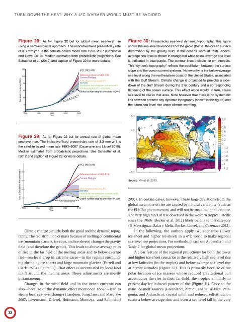Sea level (cm above 2000) 125 100 75 50 25 0 Fixed present-day rate IPCC SRES A1FI Reference (close to SRES A1B) Current Pledges 50% chance to exceed 2°C RCP3PD Illustrative low-emission scenario with strong negative CO 2 emissions Global sudden stop to emissions in 2016 Figure 30: Present-day sea-level dynamic topography. This figure shows the sea-level deviations from the geoid (that is, the ocean surface determined by the gravity field, if the oceans were at rest). Aboveaverage sea-level is shown in orange/red while below-average sea level is indicated in blue/purple. The contour lines indicate 10 cm intervals. This “dynamic topography” reflects the equilibrium between the surface slope and the ocean current systems. Noteworthy is the below-average sea level along the northeastern coast of the United States, associated with the Gulf Stream. Climate change is projected to provoke a slowdown of the Gulf Stream during the 21st century and a corresponding flattening of the ocean surface. This effect alone would, in turn, cause sea level to rise in that area. Note however that there is no systematic link between present-day dynamic topography (shown in this figure) and the future sea-level rise under climate warming. -25 1900 1950 2000 2050 2100 Year Figure 29: As for Figure 22 but for annual rate of global mean sea-level rise. The indicative/fixed present-day rate of 3.3 mm.yr-1 is the satellite based mean rate 1993–2007 (Cazenave and Llovel 2010). Median estimates from probabilistic projections. See Schaeffer et al. (2012 and caption of Figure 22 for more details. IPCC SRES A1FI Rate of Sea Level Rise (mm/year) 20 15 10 5 Fixed present-day rate 0 1900 1950 2000 2050 2100 Year Reference (close to SRES A1B) Current Pledges 50% chance to exceed 2°C RCP3PD Illustrative low-emission scenario with strong negative CO 2 emissions Global sudden stop to emissions in 2016 Climate change perturbs both the geoid and the dynamic topography. The redistribution of mass because of melting of continental ice (mountain glaciers, ice caps, and ice sheets) changes the gravity field (and therefore the geoid). This leads to above-average rates of rise in the far field of the melting areas and to below-average rise—sea-level drop in extreme cases—in the regions surrounding shrinking ice sheets and large mountain glaciers (Farrell and Clark 1976) (Figure 31). That effect is accentuated by local land uplift around the melting areas. These adjustments are mostly instantaneous. Changes in the wind field and in the ocean currents can also—because of the dynamic effect mentioned above—lead to strong local sea-level changes (Landerer, Jungclaus, and Marotzke 2007; Levermann, Griesel, Hofmann, Montoya, and Rahmstorf Source: Yin et al. 2010. 2005). In certain cases, however, these large deviations from the global mean rate of rise are caused by natural variability (such as the El Niño phenomenon) and will not be sustained in the future. The very high rates of rise observed in the western tropical Pacific since the 1960s (Becker et al. 2012) likely belong to this category (B. Meyssignac, Salas y Melia, Becker, Llovel, and Cazenave 2012). In the following, the authors apply two scenarios (lower ice-sheet and higher ice-sheet) in a 4°C world to make regional sea-level rise projections. For methods, please see Appendix 1 and Table 2 for global-mean projections. A clear feature of the regional projections for both the lower and higher ice-sheet scenarios is the relatively high sea-level rise at low latitudes (in the tropics) and below-average sea-level rise at higher latitudes (Figure 32). This is primarily because of the polar location of ice masses whose reduced gravitational pull accentuates the rise in their far-field, the tropics, similarly to present-day ice-induced pattern of rise (Figure 31). Close to the main ice-melt sources (Greenland, Arctic Canada, Alaska, Patagonia, and Antarctica), crustal uplift and reduced self-attraction cause a below-average rise, and even a sea-level fall in the very 32
Page 1 and 2: Turn Down the Heat Why a 4°C Warme
Page 3 and 4: © 2012 International Bank for Reco
Page 5 and 6: Turn Down the Heat: Why a 4°C Warm
Page 10 and 11: Foreword It is my hope that this re
Page 13 and 14: Executive Summary
Page 21 and 22: Chapter 1
Page 23: Turn Down the Heat: Why a 4°C Warm
Page 26 and 27: Observed Climate Changes and Impact
Page 42 and 43: 21st Century Projections This secti
Page 44 and 45: 21st Century Projections technologi
Page 46 and 47: 21st Century Projections Figure 23:
Page 48 and 49: 21st Century Projections A differen
Page 50 and 51: Focus: Sea-level Rise Projections P
Page 54 and 55: Focus: Sea-level Rise Projections F
Page 77: Turn Down the Heat: Why a 4°C Warm
Page 80 and 81: System Interaction and Non-linearit
Page 87 and 88: Appendix 1
Page 91 and 92: Appendix 2
Page 93 and 94: Bibliography
Page 103 and 104:
Turn Down the Heat: Why a 4°C Warm
Page 105:
Turn Down the Heat: Why a 4°C Warm
show all

Heat

You also want an ePaper? Increase the reach of your titles

Delete template?

Save as template?