Quantitative analysis of EEG signals: Time-frequency methods and ...

in this chapter, the question of a deterministic or noisy nature of EEG signals keep the
attention of many research groups during the last years.
5.2.3 Calculation of the Correlation Dimension
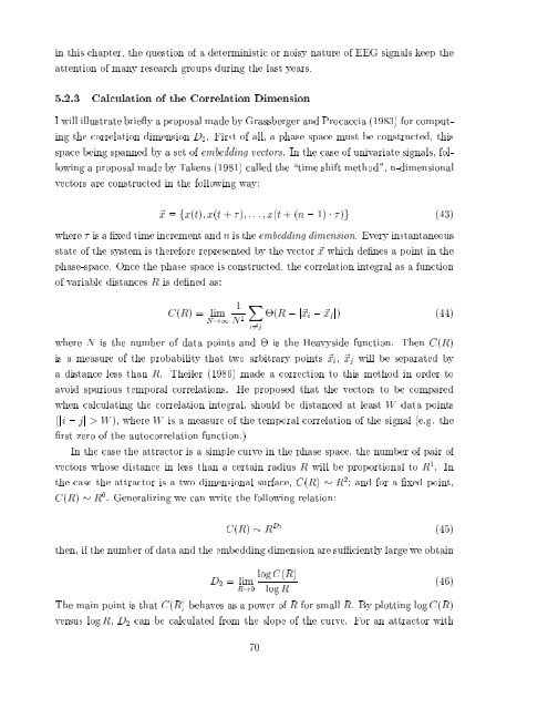
I will illustrate briey a proposal made by Grassberger and Procaccia (1983) for computing
the correlation dimension D 2 . First of all, a phase space must be constructed, this
space being spanned by a set of embedding vectors. In the case of univariate signals, following
a proposal made by Takens (1981) called the \time shift method", n-dimensional
vectors are constructed in the following way:
~x = fx(t)x(t + ):::x(t +(n ; 1) )g (43)
where is a xed time increment and n is the embedding dimension. Every instantaneous
state of the system is therefore represented by thevector ~x which denes apoint in the
phase-space. Once the phase space is constructed, the correlation integral as a function
of variable distances R is dened as:
C(R) = lim
N!1
1 X
(R ;j~x
N 2 i ; ~x j j) (44)
i6=j
where N is the number of data points and is the Heavyside function. Then C(R)
is a measure of the probability that two arbitrary points ~x i , ~x j will be separated by
a distance less than R. Theiler (1986) made a correction to this method in order to
avoid spurious temporal correlations. He proposed that the vectors to be compared
when calculating the correlation integral, should be distanced at least W data points
(ji ; jj >W), where W is a measure of the temporal correlation of the signal (e.g. the
rst zero of the autocorrelation function.)
In the case the attractor is a simple curve in the phase space, the number of pair of
vectors whose distance in less than a certain radius R will be proportional to R 1 . In
the case the attractor is a two dimensional surface, C(R) R 2 and for a xed point,
C(R) R 0 . Generalizing we can write the following relation:
C(R) R D 2
(45)
then, if the number of data and the embedding dimension are suciently large we obtain
D 2 = lim
R!0
log C(R)
log R
The main point isthatC(R) behaves as a power of R for small R. By plotting log C(R)
versus log R, D 2 can be calculated from the slope of the curve. For an attractor with
70
(46)