Conformal Geometric Algebra in Stochastic Optimization Problems ...

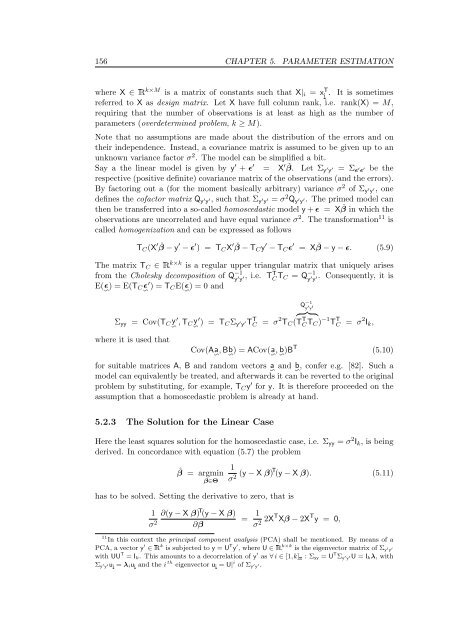
156 CHAPTER 5. PARAMETER ESTIMATION
where X ∈ �k×M is a matrix of constants such that X|i = xT i . It is sometimes
referred to X as design matrix. Let X have full column rank, i.e. rank(X) = M,
requiring that the number of observations is at least as high as the number of
parameters (overdetermined problem, k ≥ M).
Note that no assumptions are made about the distribution of the errors and on
their independence. Instead, a covariance matrix is assumed to be given up to an
unknown variance factor σ 2 . The model can be simplified a bit.
Say a the linear model is given by y ′ + ǫ ′ = X ′ β. ˇ Let Σy ′ y ′ = Σǫ ′ ǫ ′ be the
respective (positive definite) covariance matrix of the observations (and the errors).
By factoring out a (for the moment basically arbitrary) variance σ2 of Σy ′ y ′, one
defines the cofactor matrix Qy ′ y ′, such that Σy ′ y ′ = σ2Qy ′ y ′. The primed model can
then be transferred into a so-called homoscedastic model y + ǫ = X ˇ β in which the
observations are uncorrelated and have equal variance σ2 . The transformation11 is
called homogenization and can be expressed as follows
TC(X ′ ˇ β − y ′ − ǫ ′ ) = TCX ′ ˇ β − TCy ′ − TCǫ ′ = X ˇ β − y − ǫ. (5.9)
The matrix TC ∈ �k×k is a regular upper triangular matrix that uniquely arises
from the Cholesky decomposition of Q −1
y ′ y ′, i.e. TT CTC = Q −1
y ′ y ′. Consequently, it is
′ ) = TCE(ǫ) = 0 and
∽
E(ǫ ∽ ) = E(TCǫ ∽
Σyy = Cov(TC y′ , TC ∽
y ∽
where it is used that
Q −1
y ′ y ′
′
) = TCΣy ′ y ′TTC = σ 2 � �� �
TC(
Cov(Aa ∽ , Bb ∽ ) = ACov(a ∽ , b ∽ )B T
T T CTC) −1 T T C = σ 2 Ik,
(5.10)
for suitable matrices A, B and random vectors a ∽ and b ∽ , confer e.g. [82]. Such a
model can equivalently be treated, and afterwards it can be reverted to the original
problem by substituting, for example, TCy ′ for y. It is therefore proceeded on the
assumption that a homoscedastic problem is already at hand.
5.2.3 The Solution for the Linear Case
Here the least squares solution for the homoscedastic case, i.e. Σyy = σ 2 Ik, is being
derived. In concordance with equation (5.7) the problem
ˆβ = argmin
β∈Θ
has to be solved. Setting the derivative to zero, that is
1
σ 2
∂(y − X β) T (y − X β)
∂β
1
σ 2 (y − X β)T (y − X β). (5.11)
= 1
σ 2 2XT Xβ − 2X T y = 0,
11 In this context the principal component analysis (PCA) shall be mentioned. By means of a
PCA, a vector y ′ ∈ � k is subjected to y = U T y ′ , where U ∈ � k×k is the eigenvector matrix of Σy ′ y ′
with UU T = Ik. This amounts to a decorrelation of y ′ as ∀ i ∈ [1,k] � : Σyy = U T Σy ′ y ′U = Ikλ, with
Σy ′ y ′ui = λiui and the i th eigenvector ui = U| i of Σy ′ y ′.