Conformal Geometric Algebra in Stochastic Optimization Problems ...

More documents

Recommendations

Info

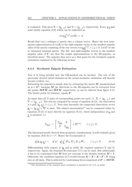
224 CHAPTER 8. APPLICATIONS IN OMNIDIRECTIONAL VISION is evaluated. This gives � = {x 1...9 } and � = {y 1...9 }, respectively. Every x-y-pair must satisfy equation (8.9) which can be rephrased as vec(x y T ) T vec(E) = 0. Recall that vec(·) reshapes a matrix into a column vector. Hence the best leastsquares approximation of vec(E) is the right-singular vector to the smallest singular value of the matrix consisting of the row vectors vec(x iy T i )T , 1 ≤ i ≤ 9. Let E ⋄ be the so estimated essential matrix. The left- and right-singular vectors to the smallest singular value of E ⋄ are then the sought approximations to the 3D-epipoles, as described above. The epipoles then serve as a first guess for the stochastic epipole estimation explained in the following section. 8.4.4 Stochastic Epipole Estimation Now it is being detailed how the GH-method can be invoked. The role of the previously derived initial estimates in the actual stochastic estimation will thereby become evident, too. Estimating the epipoles is simply done by estimating the motor M, parameterized by p ∈ � 8 : knowing M the directions to the 3D-epipoles can be extracted from the points MF � M and � MFM, respectively, as can be inferred from figure 8.14. The former point, for instance, equals F ′ . As input data all N pairs of corresponding points are used, i.e. � := {x 1...N } and � := {y 1...N }. The sets are computed by means of equation (8.12). An observation is a pair (x i, y i ), 1 ≤ i ≤ N. Note that internally the compound observation vector b i := [x i;y i ] ∈ � 6 is used. The related uncertainties 11 can be computed either by equation (8.12) or more directly by equation (8.11), where independence of x i and y i is assumed, i.e. Σbi,bi = ⎡ 0 ⎣ Σxixi 0 Σy y i i ⎤ ⎦ ∈ � 6×6 , 1 ≤ i ≤ N. The functional model, derived from geometric considerations, is self-evidently given by equation (8.8) for t = t ⋄ . Hence the G-constraint is g t i (p,x i, y i ) = p r p s x k i y l i Ot kc G a rl G c ab R b s, 1 ≤ i ≤ N, (8.13) Differentiating with respect to b i and p yields the required matrices V and U, respectively. Again, the standard H-constraint (7.7) can be used. But additionally it has to be constrained that M does not converge to the identity element M = 1. Otherwise, the condition equation (8.7) would become G = F ∧ X ∧ F ∧ Y being zero at all times. This is achieved by constraining the e-component of F ′ = MF � M, 11 The distribution of the acquired pixel coordinates is assumed to be i.i.d., as usual.
8.4. ESTIMATING EPIPOLES 225 F = eo, to be 0.5. Thus the distance d between F and F ′ is set to one12 . The needed conformal geometric algebra expression is simply d 2 � = −2eo · (M eo � � M) if M was an outright motor. In the iterative estimation process M must effectively be considered a general multivector with structural restrictions imposed by the RBM mask (7.4). Using the matrix representation of CGA, as outlined in chapter 6, a motor p = Φ(M) has the structure ⎡ ⎤ ⎢ M ≡ ⎢ ⎣ p1 + p7 −p4 − p8 p3 + p5 −p2 + p6 −p7 p8 −p5 −p6 p4 + p8 p1 + p7 p2 − p6 p3 + p5 −p8 −p7 p6 −p5 −p3 + p5 −p2 − p6 p1 − p7 p4 − p8 −p5 p6 p7 p8 p2 + p6 −p3 + p5 −p4 + p8 p1 − p7 −p6 −p5 −p8 p7 p7 −p8 p5 p6 p1 − p7 −p4 + p8 p3 − p5 −p2 − p6 p8 p7 −p6 p5 p4 − p8 p1 − p7 p2 + p6 p3 − p5 p5 −p6 −p7 −p8 −p3 − p5 −p2 + p6 p1 + p7 p4 + p8 p6 p5 p8 −p7 p2 − p6 −p3 − p5 −p4 − p8 p1 + p7 This makes it possible to derive the constraint via simple matrix calculations. Since, in the present case, M eo � M can only give vector and 5-vector components, the anti-commutator can be used to expand the inner product as Q := −2eo · (M eo � M) = −(eoM eo � M + M eo � M eo). (8.14) In CGA the reverse operation always amounts to negating the 20 bivector and trivector components of a multivector. Hence � M can be obtained by applying a sign change to the components {p 2...7 } in the above M-matrix. Evaluating equation (8.14) gives a multivector Q with only three non-zero components in q = Φf(Q): q1 : 4(p 2 5 + p2 6 + p2 7 + p2 8 ) q27 : 2(p1p8 − p2p5 − p3p6 − p4p7) q28 : −q27 ! = 1 ! = 0 ! = 0. The rightmost column shows the value the component should take. Note that the last two constraints are already part of the M � M = 1 constraint (7.6), cf. page 196. Adding the constraint p2 5 + p26 + p27 + p28 = 1/4 and differentiating ultimately gives ⎡ ⎤ ⎢ H(p) = 2⎢ ⎣ p1 p2 p3 p4 0 0 0 0 0 0 0 0 p5 p6 p7 p8 p8 −p5 −p6 −p7 −p2 −p3 −p4 p1 It remains to enlighten the usage of the pre-estimated 3D-epipoles. But this issue coincides with the requirement to provide an initial estimate for the GH-method: the initial estimate for p is the unit length translator TE - being a special motor - along the direction of the initial estimate for the 3D-epipole E from section 8.4.3, i.e. p [0] := Φ(TE). 12 This can be done as the true distance between F and F ′ cannot be recovered from the image data. ⎥ ⎦ . ⎥ . ⎥ ⎦
Page 1 and 2:
INSTITUT FÜR INFORMATIK Conformal
Page 3 and 4:
Conformal Geometric Algebra in Stoc
Page 5:
Dedicated to my beloved wife, Steph
Page 9:
ACKNOWLEDGMENT This thesis as is ca
Page 12 and 13:
3 The Conformal Geometric Algebra 8
Page 14 and 15:
8 Applications in Omnidirectional V
Page 16 and 17:
2 CHAPTER 1. INTRODUCTION with a si
Page 18 and 19:
4 CHAPTER 1. INTRODUCTION three poi
Page 20 and 21:
6 CHAPTER 1. INTRODUCTION Spherical
Page 22 and 23:
8 CHAPTER 1. INTRODUCTION Fig. 1.3:
Page 24 and 25:
10 CHAPTER 1. INTRODUCTION incidenc
Page 26 and 27:
12 CHAPTER 1. INTRODUCTION tabular
Page 28 and 29:
14 CHAPTER 1. INTRODUCTION
Page 30 and 31:
16 CHAPTER 2. GEOMETRIC ALGEBRA Gra
Page 32 and 33:
18 CHAPTER 2. GEOMETRIC ALGEBRA and
Page 34 and 35:
20 CHAPTER 2. GEOMETRIC ALGEBRA 2.1
Page 36 and 37:
22 CHAPTER 2. GEOMETRIC ALGEBRA fur
Page 38 and 39:
24 CHAPTER 2. GEOMETRIC ALGEBRA Fig
Page 40 and 41:
26 CHAPTER 2. GEOMETRIC ALGEBRA Fig
Page 42 and 43:
28 CHAPTER 2. GEOMETRIC ALGEBRA Ret
Page 44 and 45:
30 CHAPTER 2. GEOMETRIC ALGEBRA dou
Page 46 and 47:
32 CHAPTER 2. GEOMETRIC ALGEBRA whe
Page 48 and 49:
34 CHAPTER 2. GEOMETRIC ALGEBRA In
Page 50 and 51:
36 CHAPTER 2. GEOMETRIC ALGEBRA 2.2
Page 52 and 53:
38 CHAPTER 2. GEOMETRIC ALGEBRA geo
Page 54 and 55:
40 CHAPTER 2. GEOMETRIC ALGEBRA fol
Page 56 and 57:
42 CHAPTER 2. GEOMETRIC ALGEBRA Def
Page 58 and 59:
44 CHAPTER 2. GEOMETRIC ALGEBRA sug
Page 60 and 61:
46 CHAPTER 2. GEOMETRIC ALGEBRA In
Page 62 and 63:
48 CHAPTER 2. GEOMETRIC ALGEBRA due
Page 64 and 65:
50 CHAPTER 2. GEOMETRIC ALGEBRA the
Page 66 and 67:
52 CHAPTER 2. GEOMETRIC ALGEBRA Cor
Page 68 and 69:
54 CHAPTER 2. GEOMETRIC ALGEBRA Pur
Page 70 and 71:
56 CHAPTER 2. GEOMETRIC ALGEBRA Pro
Page 72 and 73:
58 CHAPTER 2. GEOMETRIC ALGEBRA Acc
Page 74 and 75:
60 CHAPTER 2. GEOMETRIC ALGEBRA Pro
Page 76 and 77:
62 CHAPTER 2. GEOMETRIC ALGEBRA it
Page 78 and 79:
64 CHAPTER 2. GEOMETRIC ALGEBRA whe
Page 80 and 81:
66 CHAPTER 2. GEOMETRIC ALGEBRA Let
Page 82 and 83:
68 CHAPTER 2. GEOMETRIC ALGEBRA Sin
Page 84 and 85:
70 CHAPTER 2. GEOMETRIC ALGEBRA Def
Page 86 and 87:
72 CHAPTER 2. GEOMETRIC ALGEBRA The
Page 88 and 89:
74 CHAPTER 2. GEOMETRIC ALGEBRA dua
Page 90 and 91:
76 CHAPTER 2. GEOMETRIC ALGEBRA It
Page 92 and 93:
78 CHAPTER 2. GEOMETRIC ALGEBRA If
Page 94 and 95:
80 CHAPTER 2. GEOMETRIC ALGEBRA
Page 96 and 97:
82 CHAPTER 3. THE CONFORMAL GEOMETR
Page 98 and 99:
Page 100 and 101:
Page 102 and 103:
Page 104 and 105:
Page 106 and 107:
Page 108 and 109:
Page 110 and 111:
Page 112 and 113:
Page 114 and 115:
100 CHAPTER 3. THE CONFORMAL GEOMET
Page 116 and 117:
Page 118 and 119:
Page 120 and 121:
Page 122 and 123:
Page 124 and 125:
Page 126 and 127:
Page 128 and 129:
Page 130 and 131:
Page 132 and 133:
Page 134 and 135:
Page 136 and 137:
Page 138 and 139:
Page 140 and 141:
Page 142 and 143:
Page 144 and 145:
Page 146 and 147:
Page 148 and 149:
Page 150 and 151:
136 CHAPTER 4. A PRIMER ON POSE EST
Page 152 and 153:
Page 154 and 155:
Page 156 and 157:
Page 158 and 159:
Page 160 and 161:
146 CHAPTER 5. PARAMETER ESTIMATION
Page 162 and 163:
Page 164 and 165:
Page 166 and 167:
Page 168 and 169:
Page 170 and 171:
Page 172 and 173:
Page 174 and 175:
Page 176 and 177:
Page 178 and 179:
Page 180 and 181:
Page 182 and 183:
Page 184 and 185:
Page 186 and 187:
Page 188 and 189: 174 CHAPTER 5. PARAMETER ESTIMATION
Page 194 and 195: 180 CHAPTER 6. PRACTICAL ASPECTS OF
Page 204 and 205: 190 CHAPTER 7. APPLICATIONS IN COMP
Page 218 and 219: 204 CHAPTER 8. APPLICATIONS IN OMNI
Page 246 and 247: 232 CHAPTER 9. CONCLUSION • The m
Page 248 and 249: 234 CHAPTER 9. CONCLUSION
Page 250 and 251: 236 APPENDIX A. SELECTED ASPECTS UN
Page 268 and 269: 254 APPENDIX B. ABBREVIATIONS
Page 270 and 271: 256 APPENDIX C. NOTATION [A;B] Vert
Page 272 and 273: 258 APPENDIX C. NOTATION
Page 274 and 275: 260 APPENDIX C. NOTATION [11] E. Ba
Page 276 and 277: 262 APPENDIX C. NOTATION [34] W. F
Page 278 and 279: 264 APPENDIX C. NOTATION [59] R. M.
Page 280 and 281: 266 APPENDIX C. NOTATION [86] D. Ni
Page 282 and 283: 268 APPENDIX C. NOTATION [113] R. S
Page 284 and 285: 270 APPENDIX C. NOTATION Conjugate,
Page 286 and 287: 272 APPENDIX C. NOTATION vision, 11
show all

Conformal Geometric Algebra in Stochastic Optimization Problems ...

Create successful ePaper yourself

Delete template?

Save as template?